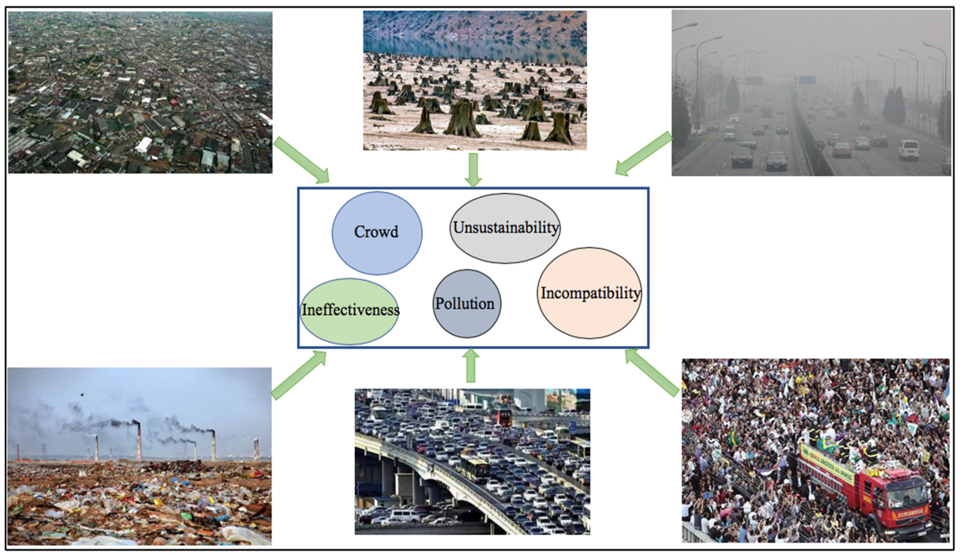
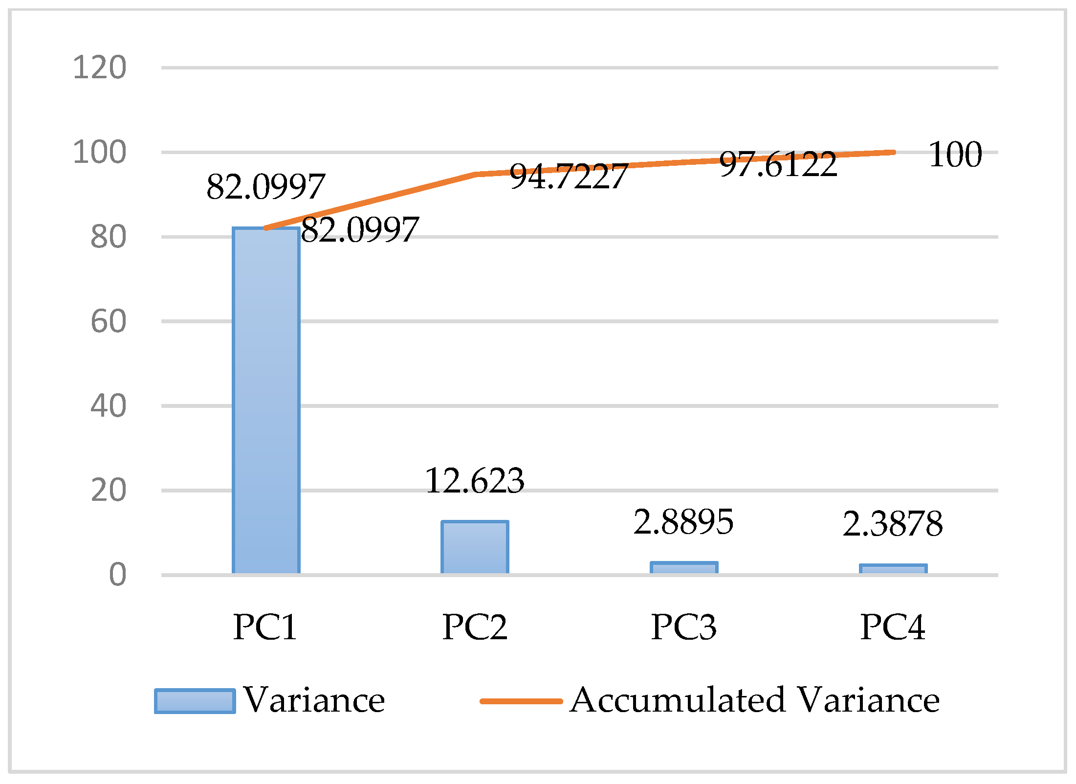
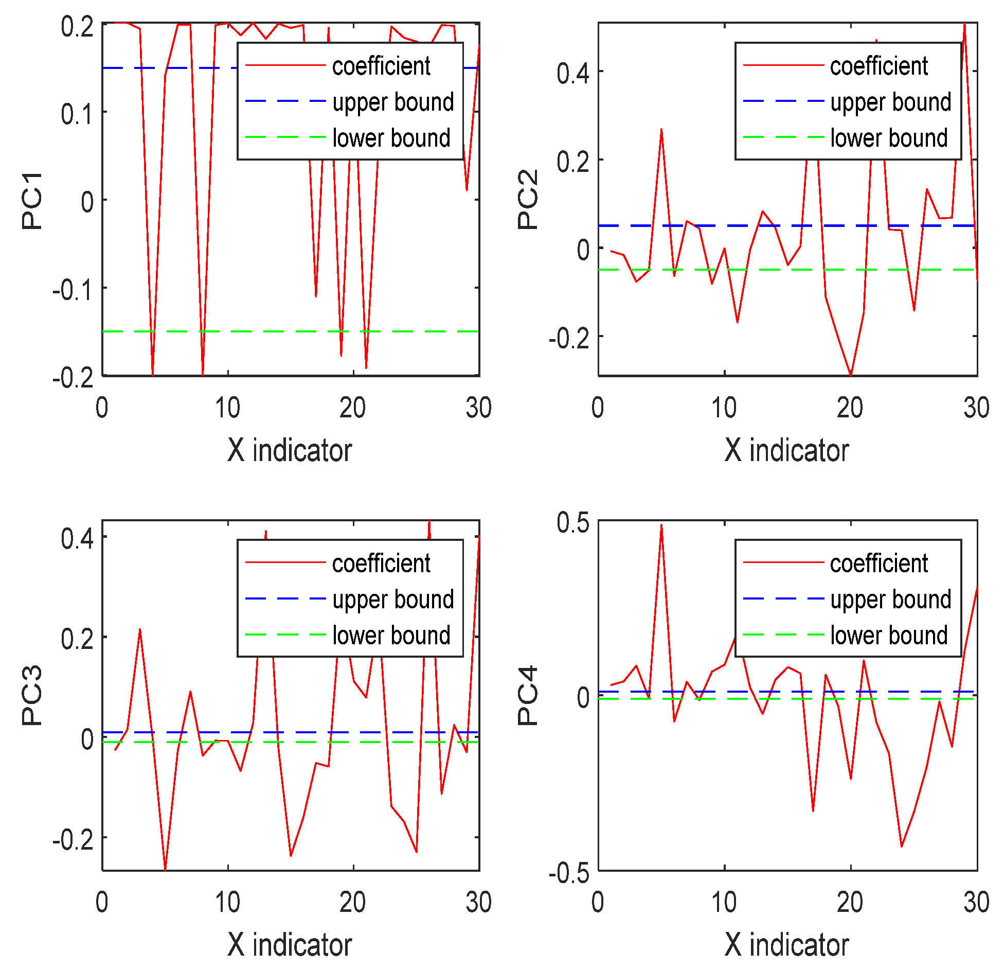
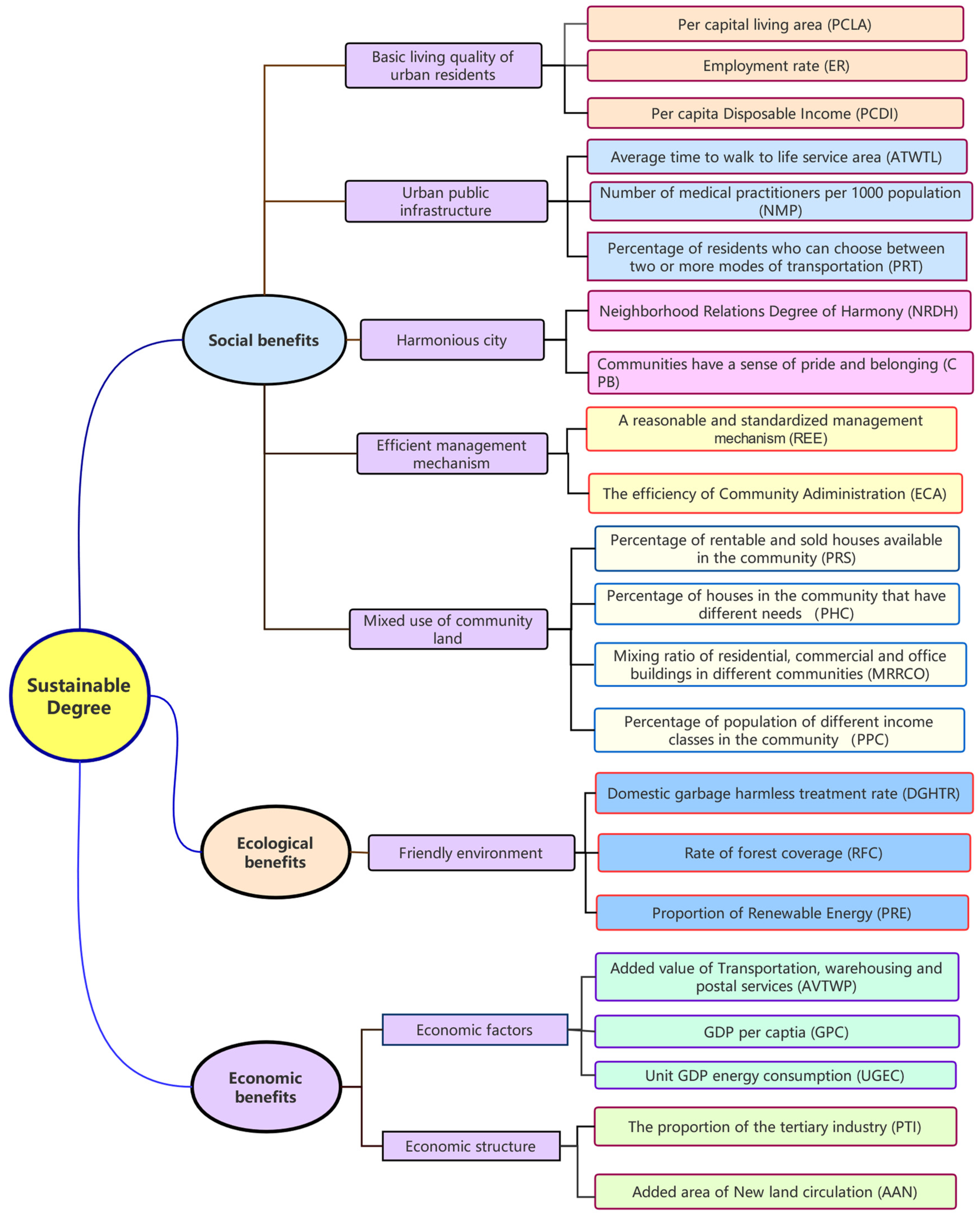
Smart growth is an advanced development mode of the economy, environment, and society. It aims to build a city with a prosperous economy, equal society, and sustainable environment [
15]. Meanwhile, 10 principles have also been clearly illustrated to guide the development of cities specifically [
11]. From a systematical view, smart growth can be defined as “the growth of economy is sustainable, the environment is suitable for living, the humanities society is more prosperous, and the consumption of natural resources can produce greater value under the minimum of environment damage, different stakeholders can participate and work together to achieve a common goal through collaboration, which all provide a high quality of life for residents.” Smart growth aims to be used to embrace a sustainable city. Therefore, sustainability is selected as the core concept in the process of constructing a conceptual framework [
29]. Then, the corresponding framework is determined subsequently.
2.2. The Evaluation Model of Sustainable Degree
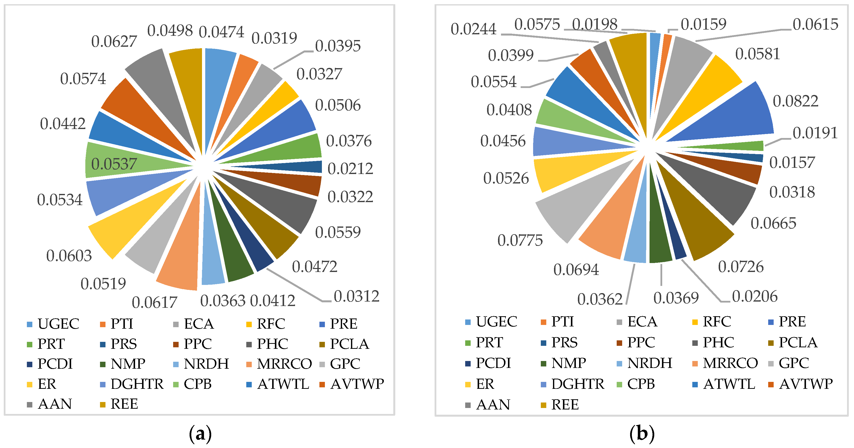
In the above context, the PCR model selects 22 indicators that have significant effects on SD. The same indicator may have different effects on different cities; an evaluated model needs to quantify these effects. Thus, the proposed model includes two parts: 1. The importance coefficient of each indicator; and 2. the weight coefficient of each indicator. Thus, the SD model can be expressed as follows:
where
is the
indicator and
.
represents the
indicator’s weight coefficient.
is the SD of the
indicator.
is the total value of the urban smart growth level.
represents the importance coefficient of the
indicator; it is carried out through mapping the element
to the interval [0,1]. The formation of
can be seen below:
Motivated by previous works [
38], the radial basis function (RBF) neural network is used to get the indicators’ weight values in this part. The RBF neural network has been widely applied to various fields in science and engineering thanks to its flexible application in high-dimensional spaces. The prominent contribution of the RBF neural network is that mapping between the input vector and hidden vector is easily conducted without weight connections [
39]. One of its universal rules is the linear assumption between the hidden layer space and output space, which can also be comprehended as summing all outputs of the hidden unit to acquire the outputs of the RBF neural network. The weight coefficient can be regarded as a flexible parameter in the network. Obviously, it is generally acknowledged that the hidden layer plays a vital key role in mapping the vector from the low dimensions to the high dimensions, so that the low-dimensional linear inseparability can become linearly separable from the high-dimensional. It is encouraging that the output layer adopts the linear optimization strategy to adjust the linear weight, thus its learning rate is rather small, and the hidden layer adopts a nonlinear optimization strategy to adjust the parameters of the activation function. The mapping of the network from the input to the output is nonlinear while the network output is linear for tunable parameters. While this method is an absolutely advanced method that can solve complex connection problems through combining linear equations, it also promotes an increased speed for learning and training. The underlying principles and procedures of the RBF neural network are shown as follows.
(1) Determine the parameters
1. Determine the initial input vector, output vector, and expected output vector:
where
is the input vector and
represents the
input layer.
is the output vector and
is the expected output vector.
is the
output layer.
2. Initialize weights between the hidden layer and the output layer:
where
is the
hidden layer.
On the basis of center initialization theory, the weight initialization method from the hidden layer to the output layer is expressed below:
where
is the minimum value of all expected outputs in the
output neuron in the training set.
is the maximum value of all expected outputs of the
output neuron in the training set.
3. Initialize the central parameters of each neuron in the hidden layer
The initial value of the center parameter of the RBF neural network is seen as below:
where
is the total number of neurons in the hidden layer,
4. Initialize the width vector
The width vector affects the range of action of neurons on input information; the smaller the width, the narrower the shape of the action function of the corresponding hidden layer neurons. Its function is shown as follows:
where
is the width adjustment coefficient; its value is less than 1. The function of
is to realize the ability to perceive and respond to local information easily and accurately.
(2) Calculate the output value,
, of the
neuron in the hidden layer:
where
is the central vector of the
neuron in the hidden layer. It is composed of the
neuron in the hidden layer corresponding to the central component of all neurons in the input layer.
is the width vector of the
neuron in the hidden layer corresponding to
.
(3) Calculate the output of neurons in the output layer:
(4) Calculate the weight coefficient
The training method for the weight parameters of the RBF neural network is the gradient descent method. Center, width, and adjusting weight parameters are adjusted to the best value by learning from adaptation, and the iterative calculation is as follows:
where
is the adjustment weight between the
output neuron and the
hidden layer neuron in the
iteration calculation.
is the adjustment weight between the
output neuron and the
hidden layer neuron in the
iterative calculation.
is the width corresponding to the center,
.
Then, the evaluation function of the RBF neural network is constructed as follows:
where
represents the evaluated result of the RBF neural network.
is the expected output value of the
output neuron in the
input sample.
is the network output value of the
output neuron in the
input sample.
(5) Calculate the
of the network output:
If , the network training is finished. Otherwise, retrain the network from Step 3.
In addition, the format of the transfer parameters is expressed in the Gaussian function (
). Apparently, the training process can be divided into two procedures. The first procedure is unsupervised learning. Its core goal is to determine the weights between the input layer and the hidden layer. The second procedure includes supervised learning and training aimed at determining the weight between the hidden layer and the output layer. As a result, the indicators’ weight values can be determined as follows:
In accordance with the above analysis,
is obtained by combining the important coefficients (
) and indicators’ weight values (
). The value of
is 0~1 while the value of
is 0~0.1, so the total value of
is 0~0.1. The evaluation criteria for
is described in
Table 4.
2.3. Prediction of the Model
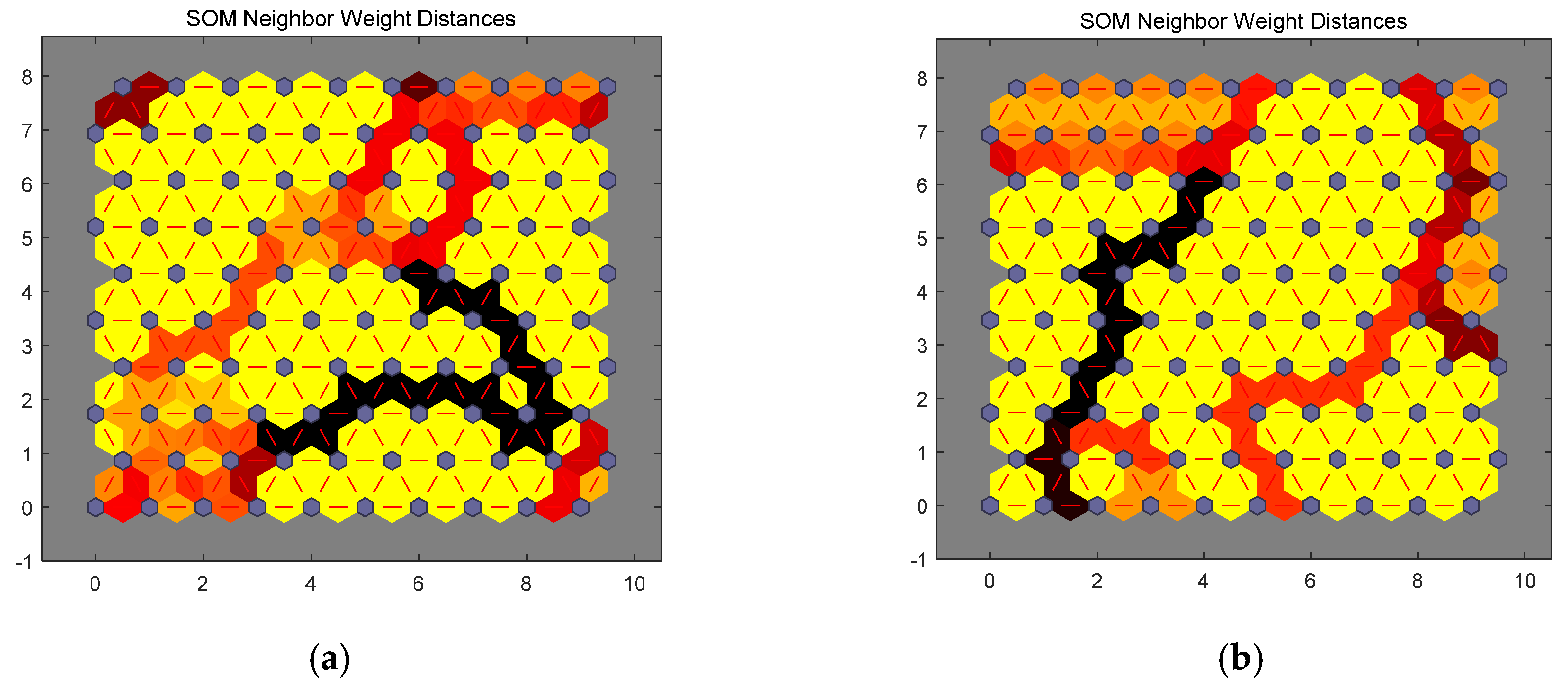
The purpose of accessing current urban development plans is to better guide the future smart growth of a city. Hence, obtaining a scientific future plan can be more useful for urban planners and policy makers. When researching the future development plans of a city, the mutual effects between future indicators should be stressed. In previous evaluation models, all indicators are processed at the same time, which can produce a certain impact on the accuracy of the model. In order to eliminate such deviation, a self-organizing map (SOM) is used to classify all indicators, and then handle them under different classifications.
An SOM is a kind of an unsupervised neural network algorithm used for clustering [
40], which has an irreplaceable position in visually analyzing data structures, it even does not need a specific output when compared to other algorithms [
41,
42]. The SOM has a special learning iterative procedure that can largely preserve the intrinsic topological features of data sets; its learning mode can be understood as a process of adjusting weights. Typically, it is constituted by an input layer and output layer. The target of the input layer is to deposit and observe the training samples while the output layer is responsible for analyzing and comparing input patterns to classify input samples. The specific training process of the SOM is shown in
Figure 5. The purple area stands for the distribution of the training data and the white grid is the extracted training data from the current distribution. First, the SOM node can be located anywhere in the data space, and the node closest to the training data (highlighted in yellow) will be chosen. Then, the SOM node moves slowly toward the training data as the expansion of neighboring nodes in the grid. At last, the white grid is consistent with the current data distribution (bottom right) through finite iterations.
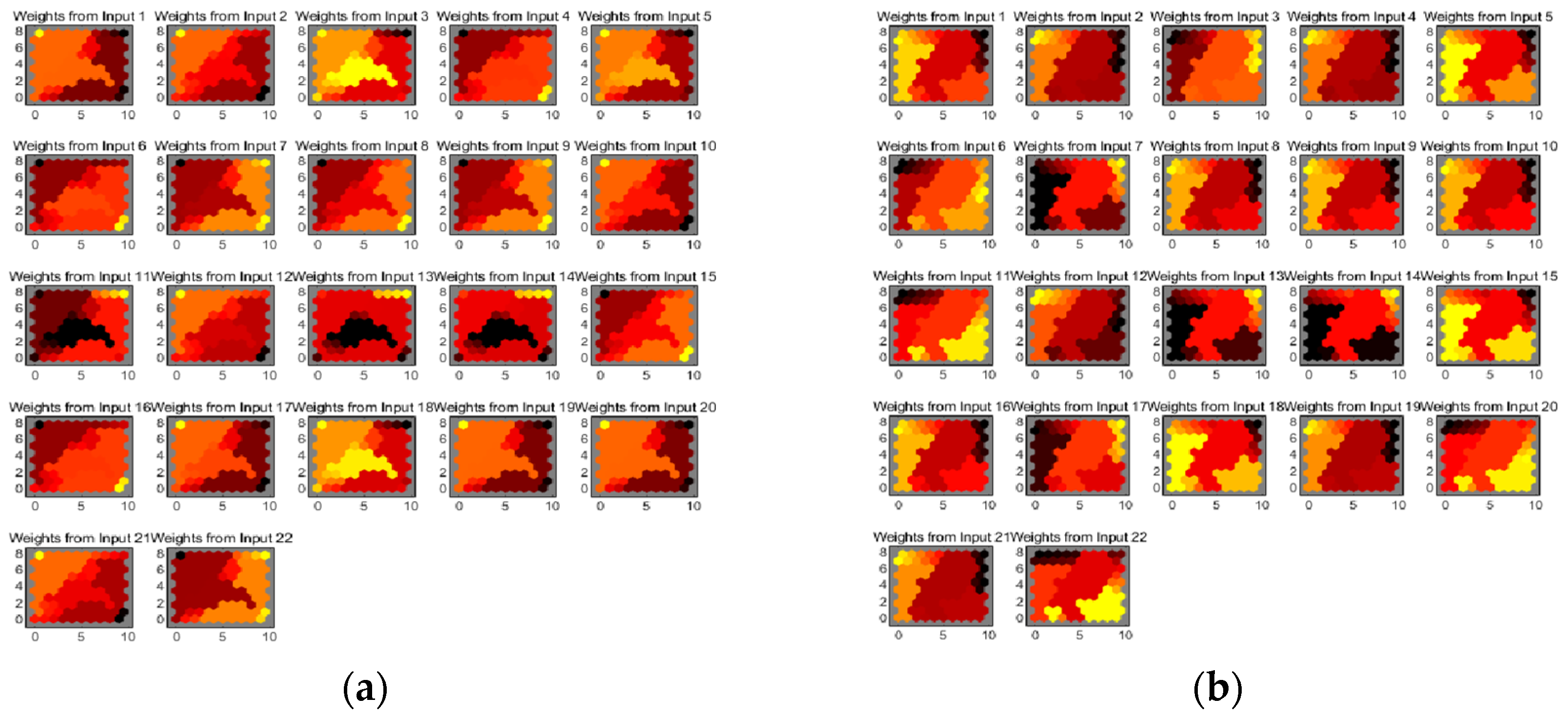
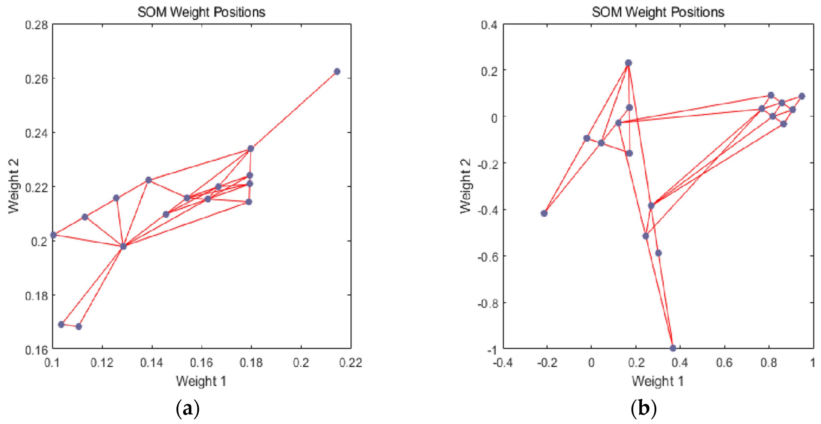
In previous studies, consideration of the best matching unit (BMU) is emphasized in the course of applying the SOM. A BMU can be comprehended as a neuron whose weight vector is close to its input. According to the direction of the input vector, which indicates the other nodes that are in the BMU neighborhood, the weight of BMU and its near neurons can be adjusted subsequently. Once the BMU is determined, the following assignment is to calculate other nodes in the BMU neighborhood until the network performance meets the specified test requirements by increasing the number of neurons, or perhaps obtaining a larger training data set. Eventually, the clustering graph is provided by MATLAB software to classify indicators.
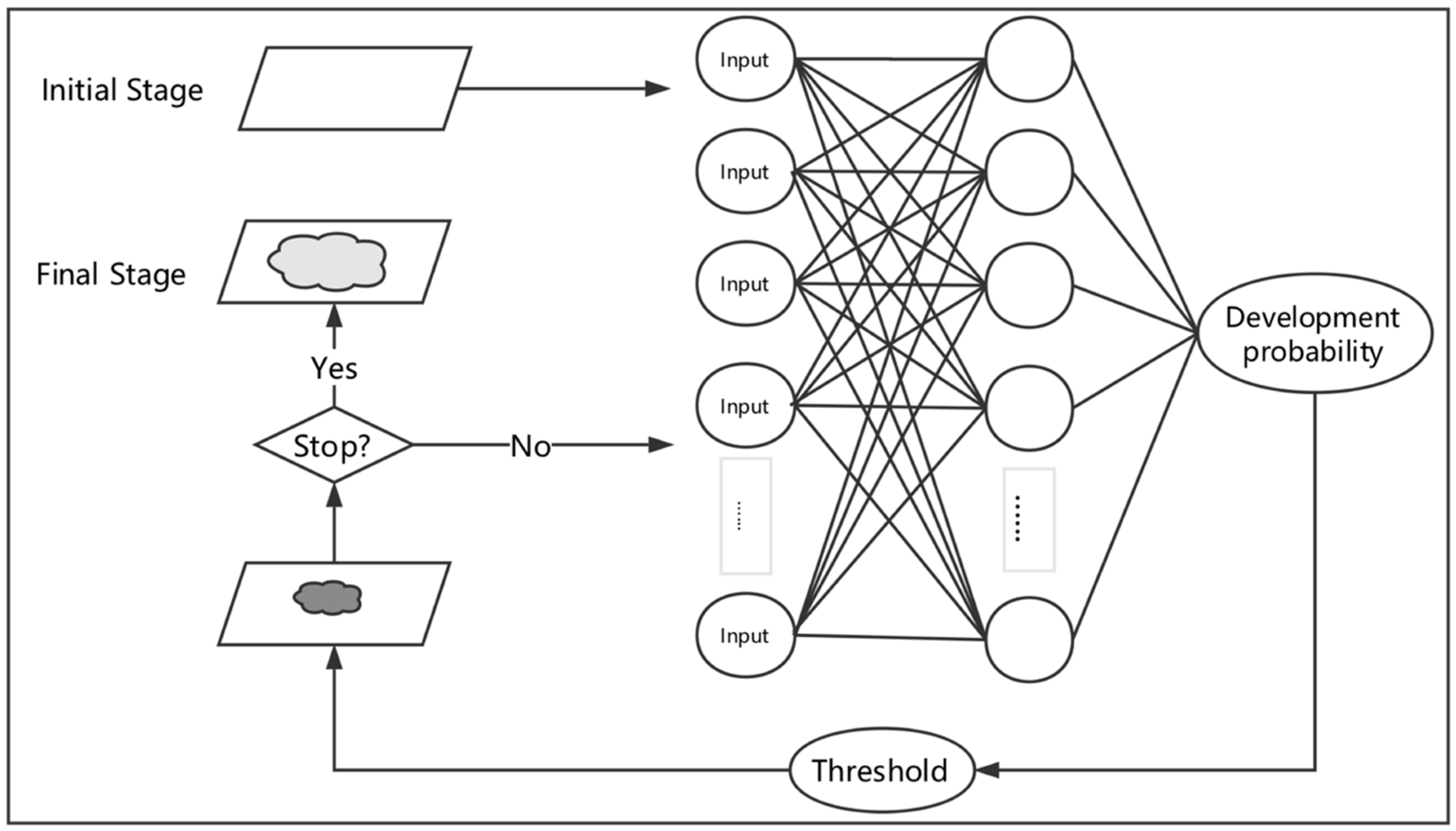
After obtaining the classification of all indicators, the SD model is used to train them under different classifications. The output of the SD is the predicted values of each indicator and the obtained changes of all indicators make up a new future plan. One major criticism is that the validity of new plans is still unknown. To overcome this difficulty, the possible tendencies of cities’ smart growth levels are simulated by cellular automata (CA) based on the new plans.
CA is a physical system model, which is composed of a cell, lattice, neighbor, and specific rules [
43]. The major function of CA is to deal with complex evolution outcomes through an ordinary rule. It can simulate the interaction between each component immediately [
44]. The conceptual diagram of the CA model is in
Figure 6.
The steps to predict the level of urban smart growth are as follows: 1. Determine the main elements of its composition, including the cell, cell space, cell state, cell neighborhood, and transformation rules; 2. analyze the urban spatial structure; 3. determine the parameters of the model, such as the reproductive parameters, diffusion parameters, propagation parameters, and constraint parameters; 4. determine the definition of the cell transformation rules required for the model; and 5. perform urban development simulation.
