Article

Optimizing Transport Scheme of High Value-Added Shipments in Regions without Express Train Services

School of Traffic and Transportation, Beijing Jiaotong University, Beijing 100044, China
*
Author to whom correspondence should be addressed.
Sustainability 2019, 11(21), 6108; https://doi.org/10.3390/su11216108
Submission received: 6 September 2019 / Revised: 23 October 2019 / Accepted: 24 October 2019 / Published: 2 November 2019
(This article belongs to the Collection Sustainable Rail and Metro Systems)

Abstract

:
In railway transportation, high value-added shipments in regions with large traffic volumes are generally delivered by express train services, since these freights need to be delivered in a short time. However, there are also high value-added shipments in areas where express train services are not available. If these freights are delivered by the traditional approaches (i.e., the freight cars are delivered to the adjacent classification yard by local trains, combined with other freight cars to form a train, and finally sent to the destination according to the transportation plan) with multiple reclassifications (a reclassification is when wagons are separated from their original train and then join another train in a classification yard), it will lead to delivery delays and economic losses to shippers and contribute to severe carbon emissions. In this context, this paper proposes an innovative method to deliver high value-added shipments in regions without express train services, which is called the method of reserving axle loads. The differences in assembling and transfer costs achieved by the method of reserving axle loads and traditional method are analyzed, especially the car-hours saved for the accumulation process of freight cars in a classification yard. Then, a corresponding mathematical model is established, which involves four scenarios: reserving axle loads for departing; reserving axle loads for arriving; reserving axle loads for both departing and arriving; and not reserving axle loads. Finally, the practicability and feasibility of the model was verified by two numerical experiments.

1. Introduction

In a railway freight system, commodities can be divided into two categories: bulk commodities (e.g., coal, ore, oil, etc.) and high value-added commodities (e.g., electronics, foods, etc.). The transportation of bulk commodities is generally less sensitive to shipping time but concerned more with shipping costs, while that of high value-added shipments is usually concerned with shipping time and punctuality.
In recent years, with the government control of carbon emissions, some goods, mostly high value-added shipments, have been shifted from roads to railways. According to statistics released by the China Railway, from 2015 to 2018, the total amount of freight transported by railway first decreased and then increased, while the number of high value-added shipments continually increased. The growth rates of high value-added shipments transported by rail were 18.7%, 25%, 9.3% and 2.3% from 2015 to 2018, respectively.
High value-added shipments are strict about the delivery time. At present, express scheduled freight trains are mainly formed between the distribution centers with large freight flows, such as the China Railway Express and the Yangtze River Express. However, it is not economical to provide express trains for scattered high value-added shipments. Therefore, how to deliver these scattered shipments quickly is an urgent problem to be solved. This paper proposes a new transportation pattern approach, namely the method of reserving axle loads (here, the “method of reserving axle loads” means that a train makes room at the departing station, so that the train can pick up some wagons at other stations), which can improve the delivery speed of high value-added shipments in regions without express train services as well as attract more high value-added shipments to the railway.
The main work and innovation points of this paper are as follows:
(i) A method using long-distance direct trains to reserve axle loads for high value-added shipments in the regions without express train service is proposed.
(ii) The accumulation cost of freight cars in reclassification yards is analyzed and deduced in detail by using the method of reserving axle loads.
(iii) Compared to the traditional method, the whole process and costs of railway transportation for high value-added shipments using the method of reserving axle loads are analyzed.
(iv) Aiming at minimizing the total cost of the whole process of transportation, a mathematical model for the high value-added shipments in regions without express train services is constructed. The model can be solved in four scenarios: reserving axle loads for departing; reserving axle loads for arriving; reserving axle loads for both departing and arriving; and not reserving axle loads. The practicability of the model was tested by two numerical examples.
The remainder of this paper is organized as follows. Section 2 summarizes the literature related to car-to-block, block-to-train and car-to-train problems. Section 3 introduces the delivery methods of general trains and express trains and puts forward the method of using the long-distance direct train to transport the high value-added shipments in the area without express train services. Section 4 analyzes the car-hours saved for the accumulation process of freight cars in a classification yard under the approach of reserving axle loads. In Section 5, a mathematical model for high value-added shipments in regions without express train services according to the method of reserving axle loads is proposed. The results of two numerical examples are presented in Section 6. Finally, concluding remarks and future research directions are given in Section 7.

2. Literature Review

To deliver high value-added shipments from regions without express train services to their destinations by train can be viewed as the car-to-train assignment problem, since it also involves the process of turning cars into a train. Generally, there are two consolidation processes at the core of the car-to-train assignment: the car-to-block assignment and the block-to-train assignment.
The car-to-block assignment problem is sometimes called the blocking plan problem, which determines how to aggregate a large number of shipments/freight cars into blocks [1]. Since the blocking plan problem is a large-scale complex combinatorial optimization problem, abundant studies have tried to solve it. A nonlinear mixed-integer programming model for the railway blocking problem was introduced by Bodin et al. [2], which is one of first models for determining a classification strategy for overall classification yards in a railway system. Newton et al. [3] extended a network design problem in which yards are represented by nodes and blocks by arcs. They then developed a branch-and-bound algorithm to solve it. Barnhart and Jin [4] formulated the railroad blocking problems as a network design problem and designed an approach to decompose the mixed integer programming problem into two simple sub-problems. Ahuja et al. [1] proposed an algorithm called the large-scale neighborhood search to solve the blocking plan problem. That algorithm can also handle a variety of practical and business constraints that are necessary for implementing a solution. They reported that the computational results obtained using real data are efficient and robust.
There are diverse mathematical models for the rail blocking problem. For example, Yaghini et al. [5] presented a mathematical formulation in which the objective is to minimize the costs of delivering all commodities. They attempted to solve that model by using a metaheuristic algorithm based on ant colony optimization and compared it with the quality of solutions generated with CPLEX software. Afterwards, the authors of [6] stated that the basic idea of the proposed algorithm is to use a simulated annealing algorithm to explore the solution space. Lin et al. [7] modeled the car-to-train problem as a bi-level programming problem, in which the upper-level finds an optimal train connection service, and the lower-level assigns each shipment to a sequence of train services and determines the frequency of services. Liu et al. [8] developed a flow assignment model for the quantitative analysis of diverting truck freight to railway and adopted a method that uses tangent lines to constitute envelope curve to linearize the model. Lin et al. [9] designed a bi-level programming model for railway network design, which can deal with empty car flow and relationships among the links in a corridor. Hasany and Shafahi [10] developed a mixed-integer program (MIP) for the railroad blocking problem and designed a new heuristic to solve the proposed model. That heuristic decomposed the model into two sub-problems of manageable size. To solve the railroad blocking problem with uncertain demand and supply resources, Hasany and Shafahi [11] developed a two-stage stochastic program model with two solution methods.
The block-to-train assignment problem determines which block will be placed on which train. Some studies were devoted to minimizing overall train complexity and the need to swap blocks en-route from one train to another. Kwon et al. [12] used a time–space network representation technique to represent car moves on sequences block-to-train assignments on a general-merchandise rail service network. The paper improved current freight car scheduling practices and described a dynamic freight car routing and scheduling. The problem was formulated as a linear multi-commodity flow problem in that paper. Similarly, Jha et al. [13] considered the block-to-train assignment problem, which is based on blocking plan and train schedule, and proposed heuristic algorithms based on the path-based formulation. Hwang and Ouyang [14] proposed a customized network assignment model for rail freight shipment demand and developed an adapted convex combination algorithm to find the shipment routing equilibrium. To minimize the sum of all expected delays and all running times, Borndörfer et al. [15] provided a mixed-integer nonlinear programming (MINLP) formulation and then used a piecewise linear approximation to reduce the MINLP to a mixed-integer linear model (MILP). Xiao et al. [16] presented a comprehensive optimization model of the formation plan to deliver all of the commodities with the minimum car-hour consumption at the technical yards which considered the one-block train and two-block train simultaneously. After the railroad blocking plan was generated, the author defined an integer programming optimization model to solve the block-to-train assignment problem. The model aimed to maximize the total cost savings of the whole railroad network compared to the single-block train service plan, where each block was allocated to a direct train service. Aiming at maximizing the total cost savings of the whole railroad network, an integer programming optimization model was defined to solve the block-to-train assignment problem by Xiao et al. [17]. In [17], the model was then improved to a path-based formulation, which had far fewer decision variables. The mathematical models developed by Lin et al. [18] meant to adjust freight flows between their shortest paths and non-shortest paths based on the 0-1 knapsack problem, which provided a new way to solve the block-to-train problem. Then, Lin et al. [19] designed a bi-level programming model that can deliver the high value-added shipments by using express scheduled train in a railway network, which provided some implications for this study.
Since the car-to-block assignment and block-to-train assignment are two continuous processes, some researchers tried to establish models to directly solve the car-to-train assignment problem. Crainic et al. [20] focused on the problems of routing freight traffic, scheduling train services and allocating classification work, and proposed a general optimization model and a heuristic algorithm for solving the multi-commodity flow problem. Haghani [21,22] made a detailed description about the empty car distribution problem and presented the formulation and solution of a combined train routing and makeup, and empty car distribution model. Keaton et al. [23] described a model about blocking and routing plans for freight cars in single carload general commodity service and used a Lagrangian relaxation technique to solve this problem. Then, Keaton [24] modeled the problem of determining optimal train connections, frequencies, and blocking and routing plans for freight cars as an all-integer linear programming problem, in which the objective was to minimize train cost, car time cost, and yard classification cost. Based on a cyclic three-layer space–time network, Zhu et al. [25] proposed a model which integrated service selection and scheduling, car classification and blocking, train makeup, and routing of time-dependent customer shipments. Considering the average travel time of trains, the energy consumption and the user satisfaction, Sun et al. [26] presented a multi-objective optimization model for train plan.
The above studies only researched the transportation problem of ordinary goods and rarely involved high value-added shipments in regions without express train services. Next, we aim at using the method of reserving axle loads to optimize the transport scheme of these high value-added shipments.

3. Problem Description

The method of reserving axle loads is an approach to shorten the delivery time of high value-added shipments without express train services. In order to better discuss this method, we need to learn about the general way of delivering freights by railway.

3.1. The Delivering Process of General Freights

General freights are generally delivered by four kinds of train services, viz. the direct train services, the through train services, the shuttle train services and the local train services. If there are enough freights between loading and unloading areas, the direct train can be operated, which will not be classified on the way. For example, general freights such as coal will be transported by direct train to the unloading site. However, some freights are too small to meet the requirements of operating direct trains. In general, the freight cars should be delivered to the adjacent classification yard by local trains, and then combined with other freight cars so that they can be sent together to the destination station according to the blocking plan. As shown in Figure 1, there are shipments to be delivered from freight station R1 to freight station R2. Firstly, the shipments will be delivered to classification yard M1 (M refers to the classification yard) by local train service LT1, and then be transported to the destination according to the blocking plan. There are three strategies in total.
i)
R1 → LT1 → DT1 → DT2 → LT2 → R2
ii)
R1 → LT1 → DT3 → DT4 → DT2 → LT2 → R2
iii)
R1 → LT1 → DT5 → DT6 → DT4 → DT2 → LT2 → R2
In strategy iii), the shipments are classified five times. In contrast, only three classification operations are needed in strategy i).
According to the farthest station rule, the wagon flow will choose a train service that can transport cars to the next classification yard as far as possible. In practice, the farthest station rule is a general way used to determine which car should choose which train service. Taking Figure 1 as an example, the freight rail cars from R1 to R2 will be delivered by strategy i) under the farthest station rule. However, due to the differences in classification times and fees at each classification yard, using the farthest station rule to deliver freight railcars may not be the optimal one. In addition, not all of the wagon flows can be transported by train services with the longest distance on account of the reclassification capacity constraints of classification yards.

3.2. The Delivering Process of High Value-Added Shipments Using Express Scheduled Trains

Because high value-added freights are sensitive to shipping time, the railway company would arrange express scheduled trains in the railway logistics center where there are large-scale shipments that need to be transported.
The express scheduled train, which is operated based on a regular timetable, is similar to the passenger train. It can be divided into three levels on the basis of the operating speed: 160, 120 and 80 km/h, while the general freight train is usually less than 50 km/h. The ways of delivering high value-added shipments by express scheduled trains mainly include the through trains (see E1 in Figure 2) and the pick-up trains (a pick-up is the placement of a block of cars into a train; see E2 in Figure 2).
Most of the high value-added shipments will be transported like E1 (see Figure 2; E1 and E2 refer to express train service), which will be classified in the railway logistics center, and then be directly shipped to L4 through E1. When the shipments of L1 (L1, L2, L3 and L4 refer to railway logistics centers) are too small to be delivered by a whole train, then the train departing from L1 will pick up some shipment cars in L2 and L3 and then be delivered to L4 directly (see E2 in Figure 2).

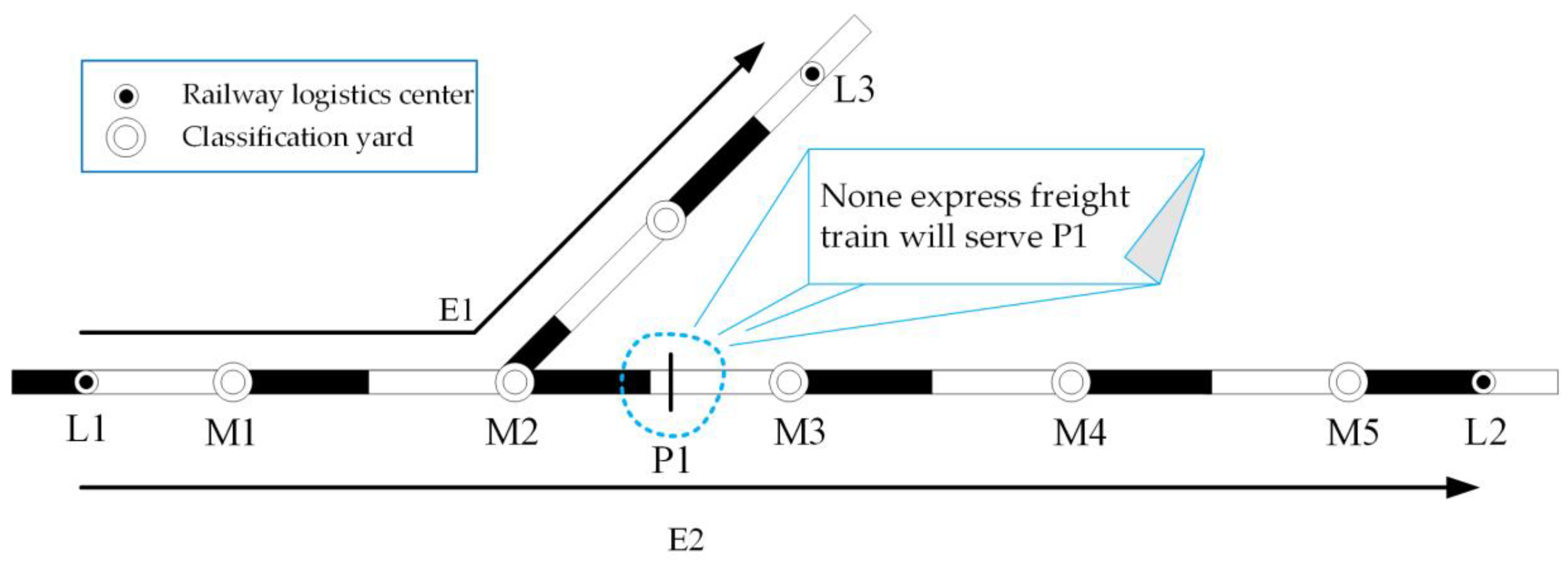
3.3. The Delivering Process of High Value-Added Shipments in Regions Without Express Train Services

A region without express train services is different from a region with express train services, which refers to the area in which the wagon flow is insufficient to operate the express scheduled train. Generally, there are two conditions:
i) None of the express scheduled trains stop at the high value-added shipments area P1 (see E1 in Figure 3).
ii) Express scheduled trains pass through the area P1 (see E2 in Figure 3).
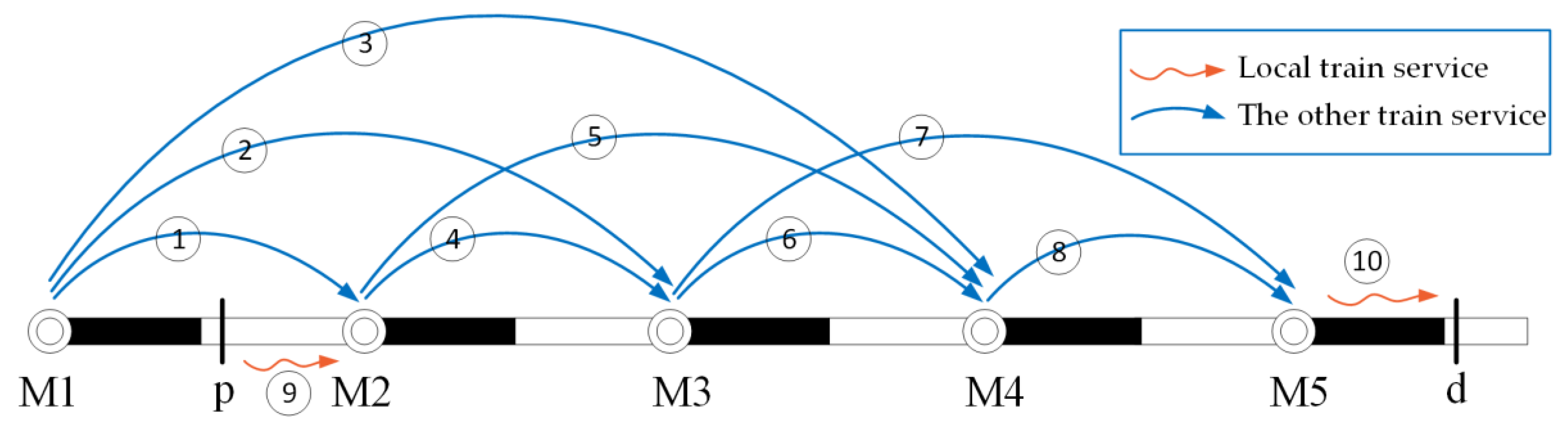
Traditionally, the high value-added shipments in the regions without express train services are usually delivered by the local train to the adjacent classification yard, and then they are delivered to the destination station according to the freight blocking plan of the railway company. Assuming that there are high value-added shipments from logistics station p to destination station d (see Figure 4), then three strategies can be adopted in the traditional method:
i)
⑨ → ④ → ⑥ → ⑧ → ⑩
ii)
⑨ → ⑤ → ⑧ → ⑩
iii)
⑨ → ④ → ⑦ → ⑩
In strategy i), the shipments need to be reclassified four times (at the classification yards M2, M3, M4 and M5). In strategy ii), the shipments need to be classified three times (at classification yard M2, M4 and M5). In strategy iii), the shipments need to be sorted three times (at the classification yards M2, M3and M5).
In the above strategies, the high value-added shipments at station p must be classified at the classification yard M2, which is the first classification yard it passes through. Can high value-added shipments be delivered more quickly and more economically if the first classification yard where these freights at station p are classified is not M2, but M3, M4 or M5? A new idea which is called reserving axle loads for high value-added shipments has been used, which is using direct trains from the classification yard M1 to pick up the high value-added freight railcars of station p.
Supposing that the railway company demands that a train cannot depart until it has 50 cars, if there are five high value-added freight cars that need to be picked up at station p, then the number of cars in the train departing from M1 will be 45 under the method of reserving axle loads. Firstly, the wagons of high value-added shipments at station p can join arc ①, arc ② or arc ③.
If arc ① is chosen, the delivering process may be ①→⑤→⑧→⑩, ①→④→⑦→⑩ or ①→④→⑥→⑧→⑩.
Similarly, if arc ② is chosen, the delivering process may be ②→⑦→⑩ or ②→⑥→⑧→⑩.
If arc ③ is chosen, the delivering process can be ③→⑧→⑩.
Suppose the delivery due date of the high value-added shipments is known. Next, we will address which arcs should be selected for high value-added shipments in regions without express train services after analyzing the time saved in the accumulation process of freight cars in the next section.

4. Time Saving in the Accumulation Process of Freight Cars at the Classification Yard Using the Method of Reserving Axle Loads

In railway transportation, trains should meet the requirements set by the railway company, e.g., a train cannot depart until 50 cars are accumulated. At the classification yard, a train is made up of several blocks which arrive at the station one after another. Therefore, the first block has to wait for the next blocks, and so it takes a certain amount of time to form a train. We define the time from the first car arriving at the classification yard to the last car arriving at the classification yard which can form a train as the accumulation cost of freight cars. This process accounts for 40%~50% of the whole operating process at the classification yard, thus it cannot be ignored.
Assuming that there is a direct train service arc DT with N Car railcars to be accumulated at the classification yard M, traditionally, the railway company requires that the size of the train (number of rail cars attached to the locomotive) running in DT is m . Let N Train denote the number of trains running in DT per day. Then, the following formula can be obtained.
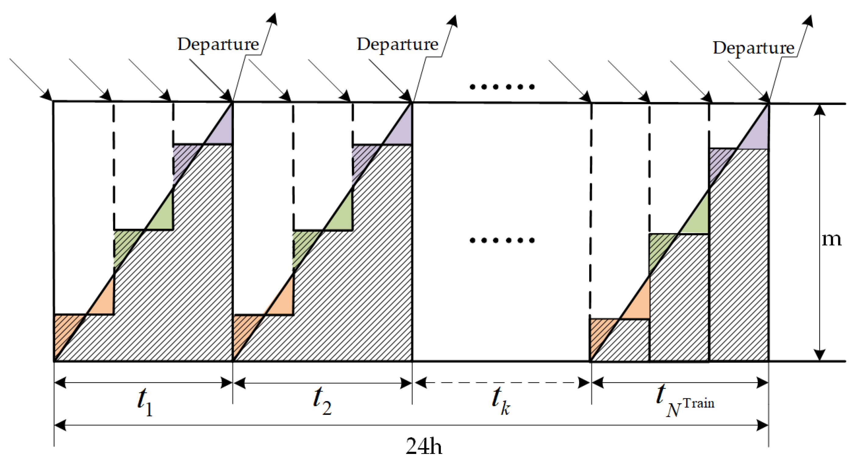
N Train = N Car m
We define T i as the car-hours incurred from the accumulation process of the freight cars of the train i , and it can be represented by the polygon area of shadow within oblique (as shown in Figure 5). When the wagon flows are equal in size and can arrive equably, the car-hours for the accumulation process of freight cars can be substituted by the triangle area based on side t i and height m .
T i = 1 2 m t i
where t i indicates the time to form the train i .
If there is no interruption among these trains, then the total car-hours T within a day can be formulated as Equation (3).
T = i 1 2 m t i = 12 m
Thus, the time of accumulation process for each car t Car is expressed in Equation (4).
t Car = 12 m N Car
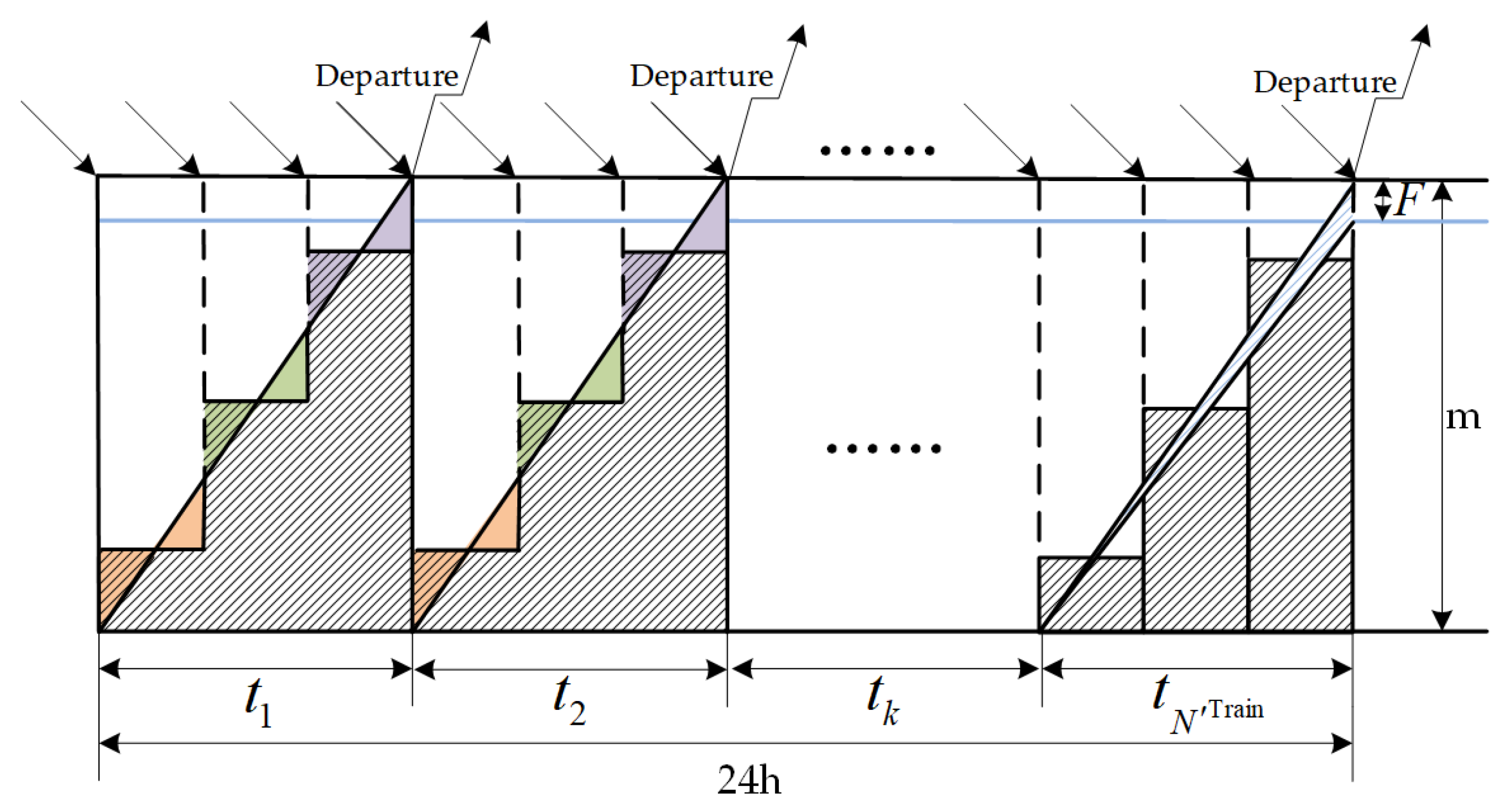
If the method of reserving axle loads is used, then the number of cars accumulated at the classification yard is not N Car but N Car F (supposing the number of high value-added freight cars waiting at station p is F ). Therefore, the car-hours for the accumulation process of freight cars can be saved. The accumulation process of freight cars using the method of reserving axle roads at the classification yard is shown in Figure 6.
Let N Train denote the number of trains running in DT per day by using the method of reserving axle loads:
N Train = N Car m + F m + 1 = N Train + F m
We define T as the total car-hours using the method of reserving axle loads.
T = 1 2 i n 1 t i m + 1 2 t n ( m F )
If the average car-hours for each train is t = 24 N Train , then Equation (6) can be written as Equation (7).
T = 1 2 t m ( N Train 1 ) + 1 2 t ( m F )
Let Δ T denote the car-hours saved per day in the accumulation process of freight cars using the method of reserving axle loads.
Δ T = T T = 12 m 1 2 t m ( N Train - 1 ) 1 2 t ( m F ) = 12 m N Car + F F
The derivation process is as follows.
Δ T = 12 m 1 2 t m ( N Train 1 ) 1 2 t ( m F ) = 12 m 1 2 t m ( N Train + F m 1 ) 1 2 t ( m F ) = 12 m 1 2 24 N Train m N Train = 12 m N Car + F F

5. Mathematical Model

The model proposed in this section aims to use long-distance direct trains to reserve axle loads for high value-added shipments without express train services. Since the mathematical model involves the method of reserving axle loads, we call it the model of reserving axle loads (Model-RAL). Now let E be the set of all stations, E 1 be the set of classification yards, S be the set of railway freight stations with high value-added shipments, and T be the set of terminal stations. Let S train = { ( i , j ) | i , j E 1 } represent the set of direct trains. Define a set S s train S train to indicate that the station s ( s S ) can be served by the train service arcs in S s train , and then define a set S t train S train to indicate that the station t ( t T ) can be served by the train service arcs in S t train .
The notations used in the mathematical model are described as follows:
Subscripts:
i , j : Subscripts of the classification yards;
s : The loading station with high value-added shipments;
t : The unloading station;
O ( s ) : The front classification yard adjacent to the station s ;
D ( t ) : The rear classification yard adjacent to the station t .
Parameters:
L i s : The distance from classification yard i to the loading station s , where i is the i in ( i , j ) S s Train ;
L t j : The distance from the unloading station t to the classification yard j , where j is the j in ( i , j ) S t Train ;
L s t : The distance from the loading station s to the unloading station t ;
N i j Car : The number of cars which originate at yard i and are destined for yard j ;
N i j Train : The frequency of direct trains which are dispatched from yard i to j ;
N O ( s ) Train : The frequency of local trains which are dispatched from s to O ( s ) ;
N D ( t ) Train : The frequency of local trains which are dispatched from D ( t ) to t ;
C s Local : Departing cost when using local trains to deliver the freights from s to O ( s ) ;
C t Local : Arriving cost when using local trains to deliver the freights from D ( t ) to t ;
C Capacity - waste : The cost per car for capacity waste of locomotive and line due to reserving axle loads;
C i Transfer : The transfer cost per car at classification yard i ;
t i Operation : The operation time per car for transfer at classification yard i ;
t s Pick - up : The stopping time of a train to pick up cars at station s ;
t t Drop - off : The stopping time of a train to drop off cars at station t ;
Δ t s Local : Additional travel time when using local trains to deliver the freights from s to O ( s ) ; note that the travel speed of the local train is lower than that of the direct train;
Δ t t Local : Additional travel time when using local trains to deliver the freights from D ( t ) to t ;
T s t : The delivery due date of high value-added shipments from s to t ;
α : Conversion factor from car-hour to fee;
v : Average travel speed of a direct train;
F : The number of cars with high value-added shipments from s to t waiting to be picked up at station s ;
m i j : The size of a normal train dispatched from i to j in the traditional method (the railway company demands that a train cannot depart until it has m i j cars);
If there are F cars from s to t at station s , then there will be m i j F cars in the train departing from the rear classification yard i .
Decision variables
x i j = { 1 Shipments   from   s   to   t   are   consolidated   into   train   service   ( i   ,   j )   at   station   s   or   yard   i 0 Otherwise
x s Local = { 1 Shipments   form   s   to   t   are   sent   from   s   to   O ( s )   by   local   train   0 Otherwise
x t Local = { 1 Shipments   from   s   to   t   are   sent   from   D ( t )   to   t   by   local   train 0 Otherwise The next step is to analyze the costs of high value-added shipments throughout the transportation process.
(1) Departing:
There are two situations according to the train services selected by cars in the departing stage.
1) The departing cost Z s Local by using local train to deliver cars from station s to the adjacent classification yard O ( s ) .
Z s Local = F C s Local x s Local
2) The departing cost Z s Direct by using direct train ( i , j ) S s Train , which consists of three parts.
(i) Savings due to reduced car-hours in the accumulation process at classification yard i ( Z i Saving )
If high value-added cars at station s choose the train service ( i , j ) S s Train , then it will save time in the accumulation process of freight cars at classification yard i . The process of that is deduced in Section 4.
Z i Saving = ( i , j ) S s Train 12 α m i j N i j Car + F F x i j
(ii) Cost of locomotive and line capacity wastes caused by reserving axle loads ( Z i s Capacity - waste )
Train service ( i , j ) reserves axle loads for high value-added shipments of express station s , which means that the train in section i s is not in a state of full axles and will cause the capacity waste of locomotive and line.
Z i s Capacity - waste = ( i , j ) S s Train C Capacity - waste F L i s x i j
(iii) Cost of the stopping delay of direct trains ( Z s Stoping - delay )
When the direct train arrives at station s , it will stop and wait for the high value-added shipments to join in. Thus, a waiting fee of the direct train is generated.
Z Stoping - delay = ( i , j ) S s Train α ( m i j F ) t s Pick - up x i j
Note that Z s Direct = Z i Saving + Z i s Capacity - waste + Z s Stoping - delay
Z s Direct = ( i , j ) S s Train [ 12 α m i j N i j Car + F F + C Capacity - waste F L i s + α ( m i j F ) t s Pick - up ] x i j
(2) Traveling:
The traveling costs include the transfer cost at the classification yard after the departure from station s (the first part of Equation (15)) and cost of travelling on the rail line (the second part of Equation (15)).
Z Traveling = F ( i , j ) S Train \ S s Train C i Transfer x i j + C Line F L s t
where C Line indicates the unit cost of a freight car running on the rail line. Since the C Line F L s t is fixed, we omit it and just consider the transfer cost.
Z Traveling = F ( i , j ) S Train \ S s Train C i Transfer x i j
(3) Arriving:
Just like departing, there are two situations.
1) The arriving cost Z t Local by using local train to transport cars from D ( t ) to t .
Z t Local = F C t Local x t Local
2) The arriving cost Z t Direct by using direct train ( i , j ) S t Train to drop off the cars at station t , which consists of two parts.
(i) Cost of locomotive and line capacity wastes in t j ( Z t j Capacity - waste )
Train service ( i , j ) drops off the high value-added cars at station t , which means that the train in section t j is not in a state of full axles and will cause the capacity waste of locomotive and line.
Z t j Capacity - waste = ( i , j ) S t Train C Capacity - waste F L t j x i j
(ii) Cost of the stopping delay of direct trains ( Z t Stoping - delay )
When the direct train arrives at station t , it will stop and drop off the high value-added cars. Thus, a waiting fee of the direct train is generated.
Z t Stoping - delay = ( i , j ) S t Train α ( m i j F ) t t Drop - off x i j
Note that Z t Direct = Z t j Capacity - waste + Z t Stoping - delay
Z t Direct = ( i , j ) S t Train [ C Capacity - waste F L t j + α ( m i j F ) t t Drop - off ] x i j
Thus, the objective function (total cost) of the Model-RAL can be expressed as follows:
min Z = Z s Local + Z s Direct + Z Traveling + Z t Local + Z t Direct = F C s Local x s Local + ( i , j ) S s Train [ 12 α m i j N i j Car + F F + C Capacity - waste F L i s + α ( m i j F ) t s Pick - up ] x i j + F ( i , j ) S Train \ S s Train C i Transfer x i j + F C t Local x t Local + ( i , j ) S t Train [ C Capacity - waste F L t j + α ( m i j F ) t t Drop - off ] x i j
Subject to
x s Local + ( i , j ) S s T r a i n x i j = 1
( i , j ) S T r a i n x i j = ( j , k ) S T r a i n x j k = 1
x t Local + ( k , h ) S t Train x k h = 1
x s Local ( Δ t s Local + 12 N O ( s ) Train ) + ( i , j ) S s Train x i j ( 12 N i j Train + t s Pick - up ) + ( i , j ) S Train \ S s Train x i j ( 12 N i j Train + t i Operation ) + L s t v + x t Local ( Δ t t Local + 12 N D ( t ) Train + t D ( t ) Operation ) T s t , F s t > 0
x s Local , x t Local , x i j { 0 , 1 } , ( i , j ) S T r a i n
The constraints in Equations (22) – (24) ensure that the high value-added shipments can be sent to the corresponding terminals. Equation (22) indicates that the high value-added shipments cars at station s can only be served by one train; Equation (23) ensures the flow balance of the stations; Equation (24) ensures that the freight cars of s t are delivered to the terminal station by only one train. The constraints in Equation (25) are bounded by the predefined due date. If Equation (25) is not satisfied, it is overdue for the high value-added shipments, then the corresponding scheme shall not be adopted. In fact, the cars with high value-added shipments cannot meet the direct train i j when they arrive at classification yard i but often need to wait for a period of time. We take the average waiting time as 12 N i j Train at classification yard i , and similarly 12 N O ( s ) Train in O ( s ) and 12 N D ( t ) Train in D ( t ) . Equation (26) presents 0–1 variables constraints.

6. Computational Experiments

6.1. Background

We take the above model into practice and present the computational results in this section. We perform computational experiments in the context of the high value-added shipments ODs, viz. from Guan (GA) to Maoming East (MME), from GA to Zhenjiang (ZJ), which travel the route Beijing–Kowloon Railway → Guangzhou–Kowloon Railway → Guangzhou–Maoming Railway → Maoming–Zhanjiang Railway, with a total length of 2479 and 2584 km, respectively, as shown in Figure 7.
The above route passes through some important classification yards (concentric circles in Figure 7), viz. Fengtai West (FTW), Hengshui (HS), Liaocheng (LC), Shangqiu North (SQN), Fuyang North (FYN), Xiangtang West (XTW) and Longchuan North (LCN). Guan (GA), the express station and Maoming East (MME) and Zhenjiang (ZJ), the terminal stations, are represented by short lines in Figure 7.
The GA station is a small express station with high value-added shipments of fertilizers and pesticides. Fertilizers and pesticides generated from Guan are mainly transported to Maoming East and Zhanjiang in spring and summer, as spring and summer are the seasons for planting and growing crops. The express trains cannot serve them because the volume of fertilizers and pesticides is relatively small and not regular in a year.

6.2. Parameters of the Model and Information on the Shipments

We adopt the method of reserving axle loads proposed in this paper, which is to use the direct train service from FTW to transport the high value-added shipments of GA. According to the transportation plan of each classification yard provided by the railway company, we draw these train service arcs in Figure 8.
The gray lines with arrows in Figure 8 represent the train service arcs among railway stations. Among them, arcs 1, 2, 3, 5, 6, 7, 8, 9, and 10 connect two classification yards; arc 4 connects GA and HS classification yard; arc 11 connects LCN classification yard and MME railway station; arc 12 connects LCN classification yard and ZJ railway station, respectively. The parameters of each arc are shown in Table 1.
Some train services in Table 1 connect two adjacent classification yards. For example, arc 6 connects LC and SQN, arc 7 connects SQN and FYN, etc. Some connect two classification yards that are not adjacent. For example, arc 1 connects FTW and LC (HS cannot be served), arc 2 connects FTW and FYN (HS, LC and SQN cannot be served), etc. Furthermore, the frequencies of trains and number of cars accumulated per day are also different among these train service arcs. For example, arc 1, ,5, 9 and 11 support four trains, which carry 200 cars per day, respectively, while arc 2 and arc 6 support five trains, which carry 250 cars per day, respectively.
There are seven classification yards with parameters shown in Table 2.
It can be seen that these classification yards have various classification fees and classification times due to the differences in facilities, layout and operation method. For example, the classification fee is 24 CNY per car and classification time is 3 hours per car for FTW, while 28 CNY per car and 4 hours per car for XTW.
For GA-MME, there are four cars with a delivery term of 64 hours on a given day (due to the unstable flow of these high value-added shipments, the daily delivery volume may not be the same, and so we take the value of a certain day); for GA-ZJ, there are five cars with a delivery term of 70 hours on a given day. The parameters of these two flows are shown in Table 3.
The other parameters are shown in Table 4.

6.3. Computational Results and Analysis

Using the data mentioned above, we solve the model by Lingo11. The parameters of the computer are Intel(R) Core(TM) i5-4200U CPU and 4 GB RAM. The above instance can be solved to optimality after running for 1 s. The optimal solution is obtained:
{ GA - MME : GA FYN LCN MME GA - ZJ : GA FYN LCN ZJ
Fertilizer and pesticide cars from GA to MME and ZJ are carried by direct train service 2 to FYN classification yard first, and then are transported to LCN classification yard by arc 9, and, finally, they are shipped from LCN to MME and ZJ, respectively. The scheme is shown in Figure 9.
The orange line represents the selected train service arc. It can be observed that the transportation schemes for GA-MME and GA-ZJ are the same as cars with fertilizers and pesticides are sent to LCN classification yard by arc 2 and arc 9, and then sent to their respective destinations from LCN. With two classifications, the transportation time for GA-MME and GA-ZJ is 58.3 hours and 64.3 hours respectively. The total cost of the scheme is 5116.5 CNY.
Next, we thoroughly study the two high value-added flows, and list all their schemes (as shown in Table 5) to analyze their differences.
There are seven schemes for each car flow (as shown in Table 5), and these schemes have different delivery times and costs since different train service arcs are selected. The freight cars of Scheme 1 and Scheme 2 are transported using the traditional method: cars with fertilizers and pesticides at GA are sent to HS classification yard by local trains and are then shipped to the terminal station (Maoming East and Zhanjiang) according to the transportation plan of HS. Due to multiple classifications, delays and costs occurred. In general, for the four cars of GA-MME and five cars of GA-ZJ, the delivery cost is sorted as: Scheme 6 < Scheme 7 < Scheme 5 < Scheme 4 < Scheme 3 < Scheme 2 < Scheme 1, and the delivery time is sorted as: Scheme 7 < Scheme 6 < Scheme 5 < Scheme 4 < Scheme 3 < Scheme 2< Scheme 1. The reason for these distinctions is that the train service arcs chosen by freight cars are different among these schemes. For example, Scheme 1 needs six classifications at classification yards, so it has the highest transportation costs and time. Scheme 6 and Scheme 7 only need to be classified twice, and therefore it can save a lot of transportation costs and time. In fact, the transportation time of Scheme 1, Scheme 2, Scheme 3 and Scheme 4 are beyond their due delivery time, and so they are not suitable, which indicates that not all reserving axle loads schemes are feasible. Scheme 6 and Scheme 7 are the ideal ways of reserving axle loads although these two schemes are slightly different. By Scheme 7, the shipments are transferred in XTW and LCN, while by Scheme 6, they are classified in FYN and LCN. With respect to the transportation costs, Scheme 6 is superior to Scheme 7; when considering transportation time, Scheme 7 is better than Scheme 6. Nevertheless, we aim to minimize the transportation cost while ensuring the predefined due date. In this way, Scheme 6 has the priority for decision.
In addition, we can draw a conclusion from Scheme 6 and Scheme 7 that using the farthest station rule cannot prove the optimal transportation scheme. With the farthest station rule, Scheme 7 will definitely be chosen (although Scheme 6 is more economical) since the first train service arc in Scheme 7 from FTW to XTW is obviously the longest arc. Scheme 6 did not choose the farthest arc in the first step, but it gets a better solution than Scheme 7. Therefore, the optimal solution may not be found by the farthest station rule, but it can be obtained through the model we proposed.
To test whether the model can easily handle a larger case, we expand the number of freight flows on the basis of the case of GA-MME and GA-ZJ. Leaving the other parameters of the rail network unchanged, two loading stations (LX, 88 km to LC, the local train frequency is 1 train/day that can carry 50 cars/day; and HZ, 105 km to SQN, the local train frequency is 2 trains/day that can carry 100 cars/day) and one unloading station (JA, 226 km from XTW, the local train frequency is 1 trains/day that can carry 50 cars/day) are added (see in Figure 10). Twenty-one freight flows are considered in this case—the parameters of which are shown in Table 6.
We keep the other parameters unchanged and test the model under the same computing environment as above. Twelve seconds passed and we obtained the following result (see Table 7).
The total cost of the scheme is 7335.23 CNY. Figure 11 visually shows how these traffic flows are transported.
On the one hand, cars from GA and LX are carried by the direct train service from FTW to FYN first, they are then transported to LCN classification yard directly, and finally they are shipped from LCN to MME and ZJ, respectively. On the other hand, cars generated from HZ are using the direct train service from LC to SQN, and then the train service from SQN to FYN, and lastly the train service from FYN to LCN. Note that the shipments generated from HZ are dropped off at station JA at last. This case prove that the model can be solved in a relatively short time by Lingo when the scale of the problem increases.

7. Conclusions and Future Work

In view of the phenomenon that high value-added shipments in regions without express train services cannot be transported through the express train and then delivery delay is often caused by the traditional transportation approach, this paper puts forward a transportation method of using the long-distance direct train to reserve axle loads for high value-added shipments. The traditional method of organizing general freights and express trains is analyzed, and the method of reserving axle loads for high value-added shipments is proposed. Then, the whole process of transportation using the method of reserving axle loads, especially the car-hours saved in the accumulation process of freight cars at the classification yard, is analyzed. Based on the proposed method, we established a mathematical model which can solve four scenarios, viz., reserving axle loads for departing; for arriving; for both departing and arriving; without reserving axle loads. The model aims to minimize the transportation cost of high value-added shipments with delivery due data constraints and several logical constraints. Finally, computational experiments on the loading stations of GA, LX and HZ and unloading stations of JA, MME and ZJ are analyzed. Two critical conclusions are drawn:
i) Using the method of reserving axle loads properly can reduce the transportation cost and accelerate the delivery speed of high value-added shipments;
ii) The remote classification rule may not bring the lowest transportation cost or the lowest delivery time for high value-added shipments.
Certainly, further study is needed before our model can be used in a large rail network since this paper only optimized the transport scheme of high value-added shipments in one direction. However, the model proposed in this paper can be used in a further study of the multi-directional transportation of high value-added shipments.

Author Contributions

Conceptualization, B.L.; methodology, B.L.; software, X.L.; validation, B.L.; formal analysis, B.L., X.L. and Z.Z.; resources, B.L.; data curation, B.L.; writing—original draft preparation, X.L. and Z.Z.; writing—review and editing, Y.Z.; visualization, X.L. and Z.Z.; supervision, Y.Z.; project administration, B.L.; funding acquisition, B.L.

Acknowledgments

This work was supported by the National Key R&D Program of China (2018YFB1201402).

Conflicts of Interest

The authors declare no conflict of interest.

References

  1. Ahuja, R.K.; Jha, K.C.; Liu, J. Solving Real-Life Railroad Blocking Problems. Interfaces 2007, 37, 404–419. [Google Scholar] [CrossRef]
  2. Bodin, L.D.; Golden, B.L.; Schuster, A.D.; Romig, W. A model for the blocking of trains. Transp. Res. Part B Methodol. 1980, 14, 115–120. [Google Scholar] [CrossRef]
  3. Newton, H.N.; Barnhart, C.; Vance, P.H. Constructing Railroad Blocking Plans to Minimize Handling Costs. Transp. Sci. 1998, 32, 330–345. [Google Scholar] [CrossRef]
  4. Barnhart, C.; Jin, H.; Vance, P.H. Railroad Blocking: A Network Design Application. Oper. Res. 2000, 48, 603–614. [Google Scholar] [CrossRef]
  5. Yaghini, M.; Foroughi, A.; Nadjari, B. Solving railroad blocking problem using ant colony optimization algorithm. Appl. Math. Model. 2011, 35, 5579–5591. [Google Scholar] [CrossRef]
  6. Yaghini, M.; Momeni, M.; Sarmadi, M. Solving train formation problem using simulated annealing algorithm in a simplex framework. J. Adv. Transport. 2014, 48, 402–416. [Google Scholar] [CrossRef]
  7. Lin, B.-L.; Wang, Z.-M.; Ji, L.-J.; Tian, Y.-M.; Zhou, G.-Q. Optimizing the freight train connection service network of a large-scale rail system. Transp. Res. Part B Methodol. 2012, 46, 649–667. [Google Scholar] [CrossRef]
  8. Liu, C.; Lin, B.; Wang, J.; Xiao, J.; Liu, S.; Wu, J.; Li, J. Flow assignment model for quantitative analysis of diverting bulk freight from road to railway. PLoS ONE 2017, 12, e0182179. [Google Scholar] [CrossRef]
  9. Lin, B.; Liu, C.; Wang, H.; Lin, R. Modeling the railway network design problem: A novel approach to considering carbon emissions reduction. Transp. Res. Part D Transp. Environ. 2017, 56, 95–109. [Google Scholar] [CrossRef]
  10. Hasany, R.M.; Shafahi, Y. Modeling Formulation and a New Heuristic for the Railroad Blocking Problem. Appl. Math. 2017, 56, 304–324. [Google Scholar] [CrossRef]
  11. Hasany, R.M.; Shafahi, Y. Two-stage stochastic programming for the railroad blocking problem with uncertain demand and supply resources. Comput. Ind. Eng. 2017, 106, 275–286. [Google Scholar] [CrossRef]
  12. Kwon, O.K.; Martland, C.D.; Sussman, J.M. Routing and scheduling temporal and heterogeneous freight car traffic on rail networks. Transp. Res. Part E Logist. Transp. Rev. 1998, 34, 101–115. [Google Scholar] [CrossRef]
  13. Jha, K.C.; Ahuja, R.K.; Sahin, G. New approaches for solving the block-to-train assignment problem. Networks 2008, 51, 48–62. [Google Scholar] [CrossRef]
  14. Hwang, T.; Ouyang, Y. Assignment of Freight Shipment Demand in Congested Rail Networks. Transp. Res. Rec. J. Transp. Res. Board 2014, 2448, 37–44. [Google Scholar] [CrossRef]
  15. Borndörfer, R.; Klug, T.; Schlechte, T.; Fügenschuh, A.; Schang, T.; Schülldorf, H. The Freight Train Routing Problem for Congested Railway Networks with Mixed Traffic. Transp. Sci. 2016, 50, 408–423. [Google Scholar] [CrossRef]
  16. Xiao, J.; Lin, B. Comprehensive optimization of the one-block and two-block train formation plan. J. Rail Transp. Plan. Manag. 2016, 6, 218–236. [Google Scholar] [CrossRef]
  17. Xiao, J.; Pachl, J.; Lin, B.; Wang, J. Solving the block-to-train assignment problem using the heuristic approach based on the genetic algorithm and tabu search. Transp. Res. Part B Methodol. 2018, 108, 148–171. [Google Scholar] [CrossRef]
  18. Lin, B.; Liu, S.; Lin, R.; Wu, J.; Wang, J.; Liu, C. Modeling the 0-1 Knapsack Problem in Cargo Flow Adjustment. Symmetry 2017, 9, 118. [Google Scholar] [CrossRef]
  19. Lin, B.; Wu, J.; Wang, J.; Duan, J.; Zhao, Y. A Bi-Level Programming Model for the Railway Express Cargo Service Network Design Problem. Symmetry 2018, 10, 227. [Google Scholar] [CrossRef]
  20. Crainic, T.; Ferland, J.-A.; Rousseau, J.-M. A Tactical Planning Model for Rail Freight Transportation. Transp. Sci. 1984, 18, 165–184. [Google Scholar] [CrossRef]
  21. Haghani, A.E. Rail freight transportation: A review of recent optimization models for train routing and empty car distribution. J. Adv. Transp. 1987, 21, 147–172. [Google Scholar] [CrossRef]
  22. Haghani, A.E. Formulation and solution of a combined train routing and makeup, and empty car distribution model. Transport. Res. B Meth. 1989, 23, 433–452. [Google Scholar] [CrossRef]
  23. Keaton, M.H. Designing optimal railroad operating plans: Lagrangian relaxation and heuristic approaches. Transp. Res. Part B Methodol. 1989, 23, 415–431. [Google Scholar] [CrossRef]
  24. Keaton, M.H. Designing Railroad Operating Plans: A Dual Adjustment Method for Implementing Lagrangian Relaxation. Transp. Sci. 1992, 26, 263–279. [Google Scholar] [CrossRef]
  25. Zhu, E.; Crainic, T.G.; Gendreau, M. Scheduled Service Network Design for Freight Rail Transportation. Oper. Res. 2014, 62, 383–400. [Google Scholar] [CrossRef]
  26. Sun, Y.; Cao, C.; Wu, C. Multi-objective optimization of train routing problem combined with train scheduling on a high-speed railway network. Transp. Res. Part C Emerg. Technol. 2014, 44, 1–20. [Google Scholar] [CrossRef]
Figure 1. The traditional delivering process.
Sustainability 11 06108 g001
Figure 2. Two ways of express scheduled trains.
Sustainability 11 06108 g002
Figure 3. Two conditions for regions without an express train.
Sustainability 11 06108 g003
Figure 4. High value-added shipments from logistics station p to destination d.
Sustainability 11 06108 g004
Figure 5. The accumulation process of freight cars which arrive evenly without interruption.
Sustainability 11 06108 g005
Figure 6. The accumulation process of freight cars with reserving axle loads.
Sustainability 11 06108 g006
Figure 7. The rail line from Fengtai West (FTW) to Zhenjiang (ZJ).
Sustainability 11 06108 g007
Figure 8. Train service arcs along the route.
Sustainability 11 06108 g008
Figure 9. The most optimal transportation scheme.
Sustainability 11 06108 g009
Figure 10. Train service arcs along the route.
Sustainability 11 06108 g010
Figure 11. The most optimal transportation scheme.
Sustainability 11 06108 g011
Table 1. Parameters of train service arcs. (Fengtai West (FTW), Hengshui (HS), Liaocheng (LC), Shangqiu North (SQN), Fuyang North (FYN), Xiangtang West (XTW), Longchuan North (LCN), Guan (GA), Maoming East (MME) and Zhenjiang (ZJ).)
No.Tail of ArcHead of Arc N i j Train N i j Car
1FTWLC4200
2FTWFYN5250
3FTWXTW6300
4GAHS2100
5HSLC4200
6LCSQN5250
7SQNFYN6300
8FYNXTW7350
9FYNLCN4200
10XTWLCN6300
11LCNMME4200
12LCNZJ2100
Table 2. Parameters of the classification yards.
No.Classification Yard C i Transfer (CNY/car) t i Operation (Hour)
1FTW243
2HS284
3LC203.5
4SQN244
5FYN244.5
6XTW284
7LCN203.5
Table 3. The parameters of the two shipments.
ParametersGA-MMEGA-ZJ
F (car)45
T s t (hour)6470
C s Local (CNY/car)300300
C t Local (CNY/car)400450
Δ t s Local (hour)33
Δ t t Local (hour)67.5
t s Pick - up (hour)0.50.5
t t Drop - off (hour)0.50.5
L i s (km)5757
L t j (km)--
L s t (km)24792584
Note that there is no classification yard beyond MME and ZJ, so the L t j is null.
Table 4. The other parameters.
ParametersValue
C Capacity - waste (CNY/car-km)0.75
α (CNY/car-hour)20
v (km/hour)70
m i j (car)50
Table 5. All the schemes of the two flows.
GA-MMEGA-ZJ
Scheme 1: 4-5-6-7-8-10-11Scheme 1: 4-5-6-7-8-10-12
Total fee3376Total fee4470
Transportation time88.03Transportation time94.03
Does it meet the delivery deadline?noDoes it meet the delivery deadline?no
Scheme 2: 4-5-6-7-9-11Scheme 2: 4-5-6-7-9-12
Total fee3264Total fee4330
Transportation time83.3Transportation time89.31
Does it meet the delivery deadline?noDoes it meet the delivery deadline?no
Scheme 3: 1-6-7-8-10-11Scheme 3: 1-6-7-8-10-12
Total fee2459.71Total fee3201.07
Transportation time75.53Transportation time81.53
Does it meet the delivery deadline?noDoes it meet the delivery deadline?no
Scheme 4: 1-6-7-9-11Scheme 4: 1-6-7-9-12
Total fee2347.71Total fee3061.07
Transportation time70.81Transportation time73.81
Does it meet the delivery deadline?noDoes it meet the delivery deadline?no
Scheme 5: 2-8-10-11Scheme 5: 2-8-10-12
Total fee2330.02Total fee3038.46
Transportation time63.03Transportation time69.03
Does it meet the delivery deadline?yesDoes it meet the delivery deadline?yes
Scheme 6: 2-9-11Scheme 6: 2-9-12
Total fee2218.02Total fee2898.46
Transportation time58.31Transportation time64.31
Does it meet the delivery deadline?yesDoes it meet the delivery deadline?yes
Scheme 7: 3-10-11Scheme 7: 3-10-12
Total fee2265.11Total fee2957.03
Transportation time56.41Transportation time62.41
Does it meet the delivery deadline?yesDoes it meet the delivery deadline?yes
Table 6. The parameters of the 21 shipments.
No. s t F
(Car)
T s t
(Hour)
C s Local
(CNY/Car)
C t Local
(CNY/Car)
Δ t s Local
(Hour)
Δ t t Local
(Hour)
t s Pick - up
(Hour)
t t Drop - off
(Hour)
L s t
(Hour)
1GAMME4 64 3004002.334.650.500.502479
2GAMME5 70 3004002.334.650.500.502479
3GAJA7 48 3005002.332.420.500.501646
4GAJA9 46 3005002.332.420.500.501646
5GAJA3 45 3005002.332.420.500.501646
6GAZJ4 70 3004502.335.780.500.502584
7GAZJ6 75 3004502.335.780.500.502584
8LXMME5 45 4004000.944.650.500.502198
9LXMME3 45 4004000.944.650.500.502198
10LXJA4 38 4005000.942.420.500.501365
11LXJA6 38 4005000.942.420.500.501365
12LXJA7 38 4005000.942.420.500.501365
13LXZJ5 48 4004500.945.780.500.502303
14LXZJ6 48 4004500.945.780.500.502303
15HZMME9 42 4504001.134.650.500.501964
16HZMME10 42 4504001.134.650.500.501964
17HZJA5 35 4505001.132.420.500.501131
18HZJA4 35 4505001.132.420.500.501131
19HZJA6 35 4505001.132.420.500.501131
20HZZJ7 45 4504501.135.780.500.502069
21HZZJ5 45 4504501.135.780.500.502069
Table 7. The schemes of the 21 shipments.
No. s t Scheme s
1GAMMEFTW (pick up at GA) → FYN → LCN → MME
2GAMMEFTW (pick up at GA) → FYN → LCN → MME
3GAJAFTW (pick up at GA) → FYN → LCN (drop off at JA)
4GAJAFTW (pick up at GA) → FYN → LCN (drop off at JA)
5GAJAFTW (pick up at GA) → FYN → LCN (drop off at JA)
6GAZJFTW (pick up at GA) → FYN → LCN → ZJ
7GAZJFTW (pick up at GA) → FYN → LCN → ZJ
8LXMMEFTW (pick up at LX) → FYN → LCN → MME
9LXMMEFTW (pick up at LX) → FYN → LCN → MME
10LXJAFTW (pick up at LX) → FYN → LCN (drop off at JA)
11LXJAFTW (pick up at LX) → FYN → LCN (drop off at JA)
12LXJAFTW (pick up at LX) → FYN → LCN (drop off at JA)
13LXZJFTW (pick up at LX) → FYN → LCN → ZJ
14LXZJFTW (pick up at LX) → FYN → LCN → ZJ
15HZMMELC (pick up at HZ) → SQN → FYN → LCN → MME
16HZMMELC (pick up at HZ) → SQN → FYN → LCN → MME
17HZJALC (pick up at HZ) → SQN → FYN → LCN (drop off at JA)
18HZJALC (pick up at HZ) → SQN → FYN → LCN (drop off at JA)
19HZJALC (pick up at HZ) → SQN →FYN → LCN (drop off at JA)
20HZZJLC (pick up at HZ) → SQN →FYN → LCN → ZJ
21HZZJLC (pick up at HZ) → SQN →FYN → LCN → ZJ

