Application of Artificial Intelligence Techniques to Predict the Well Productivity of Fishbone Wells


Abstract
1. Introduction
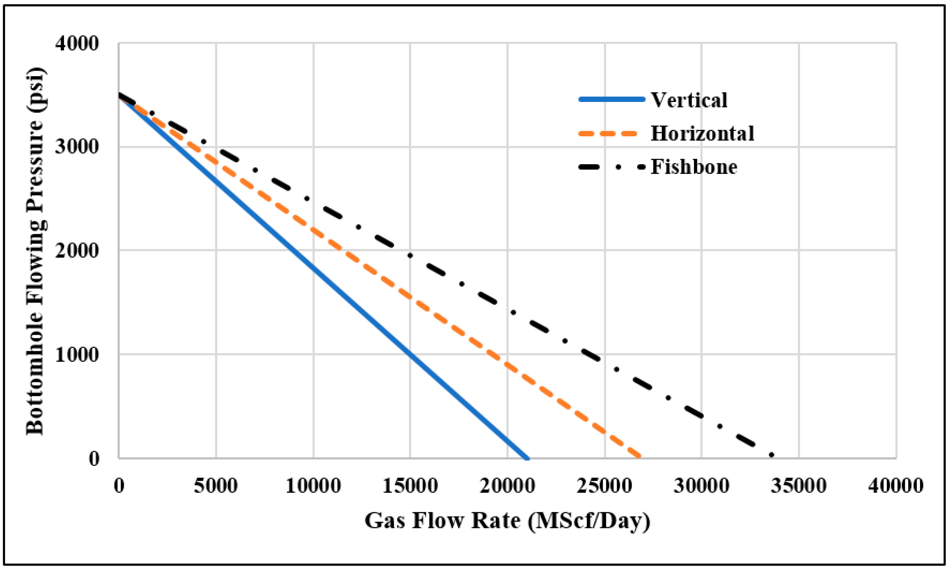
1.1. Inflow Performance Relationship
1.2. Artificial Intelligence Techniques
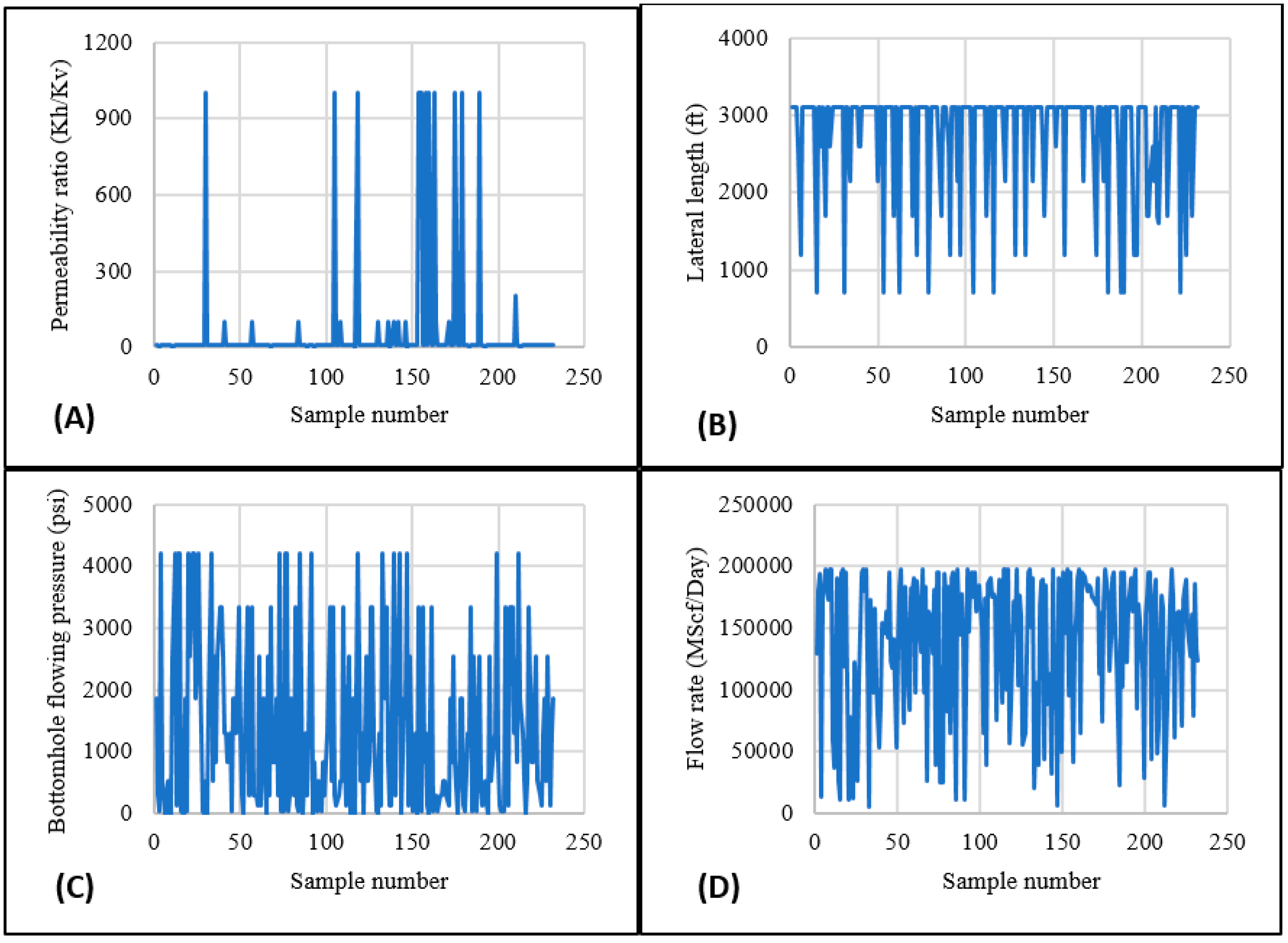
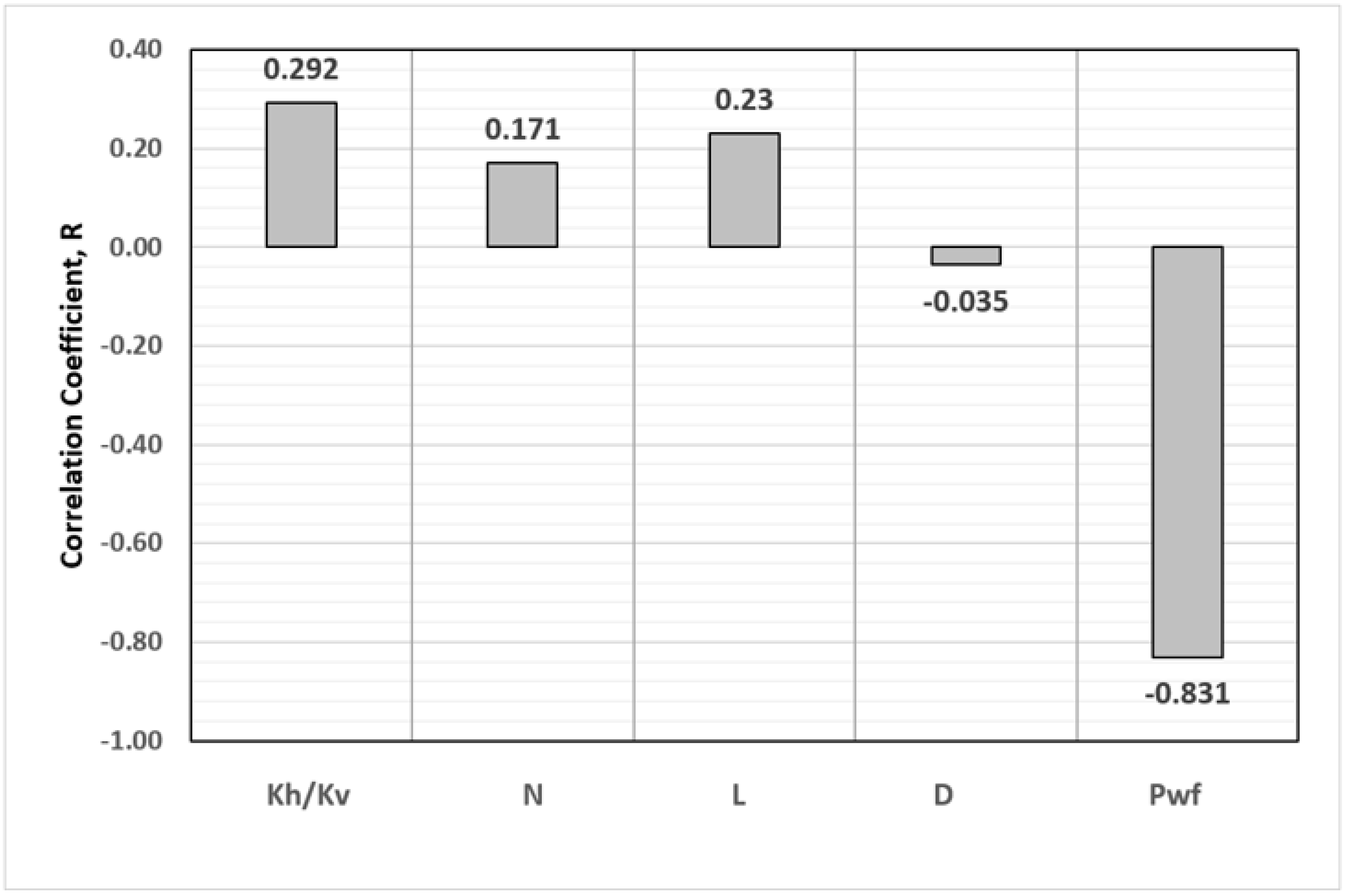
2. Data Acquisition and Analysis
3. Results and Discussion
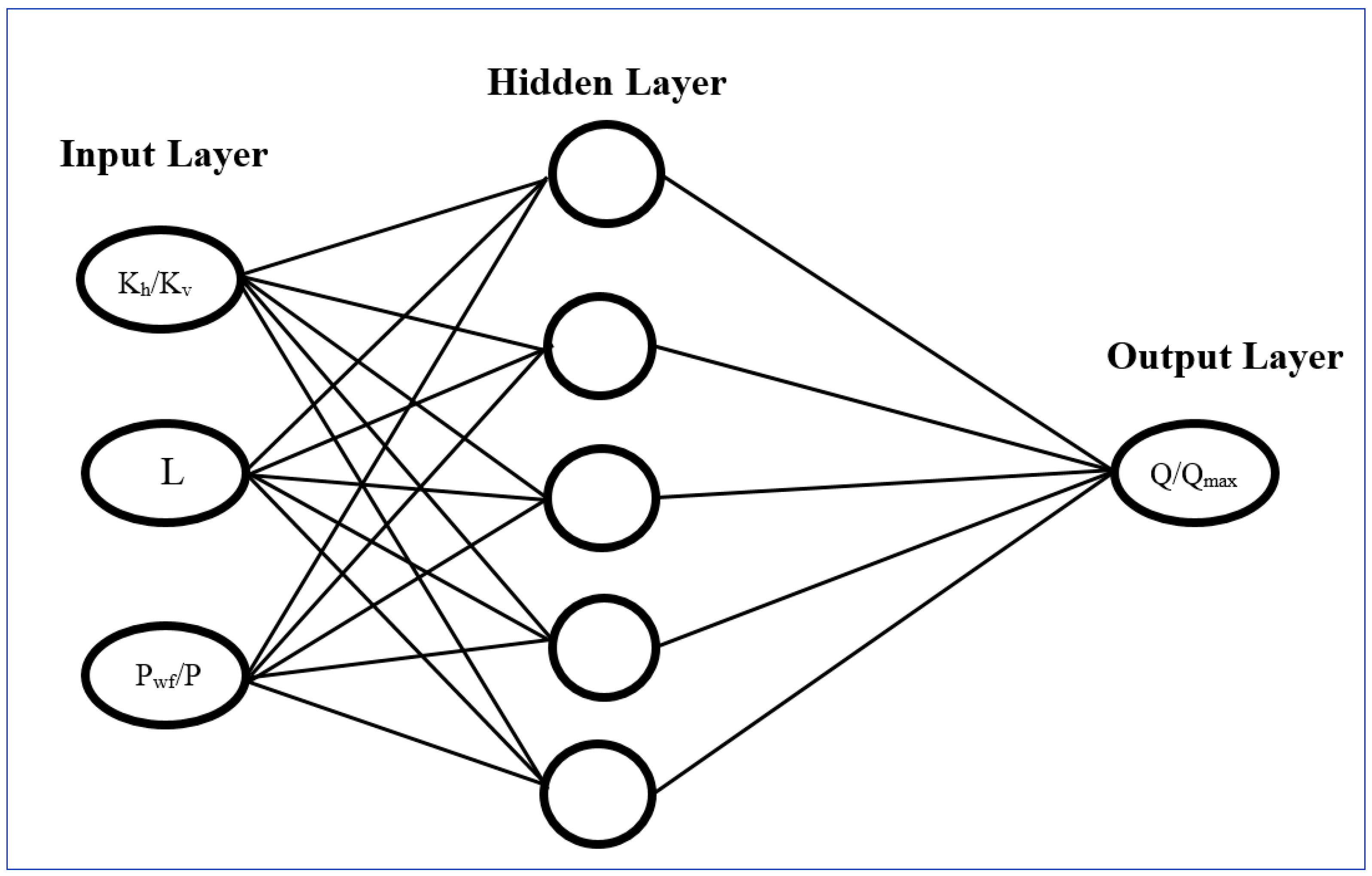
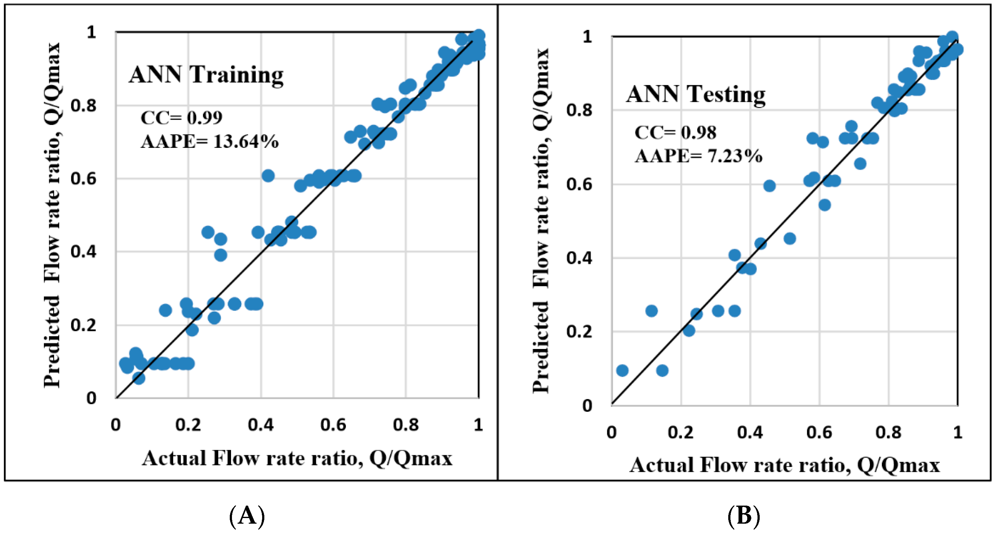
3.1. Artificial Neural Network
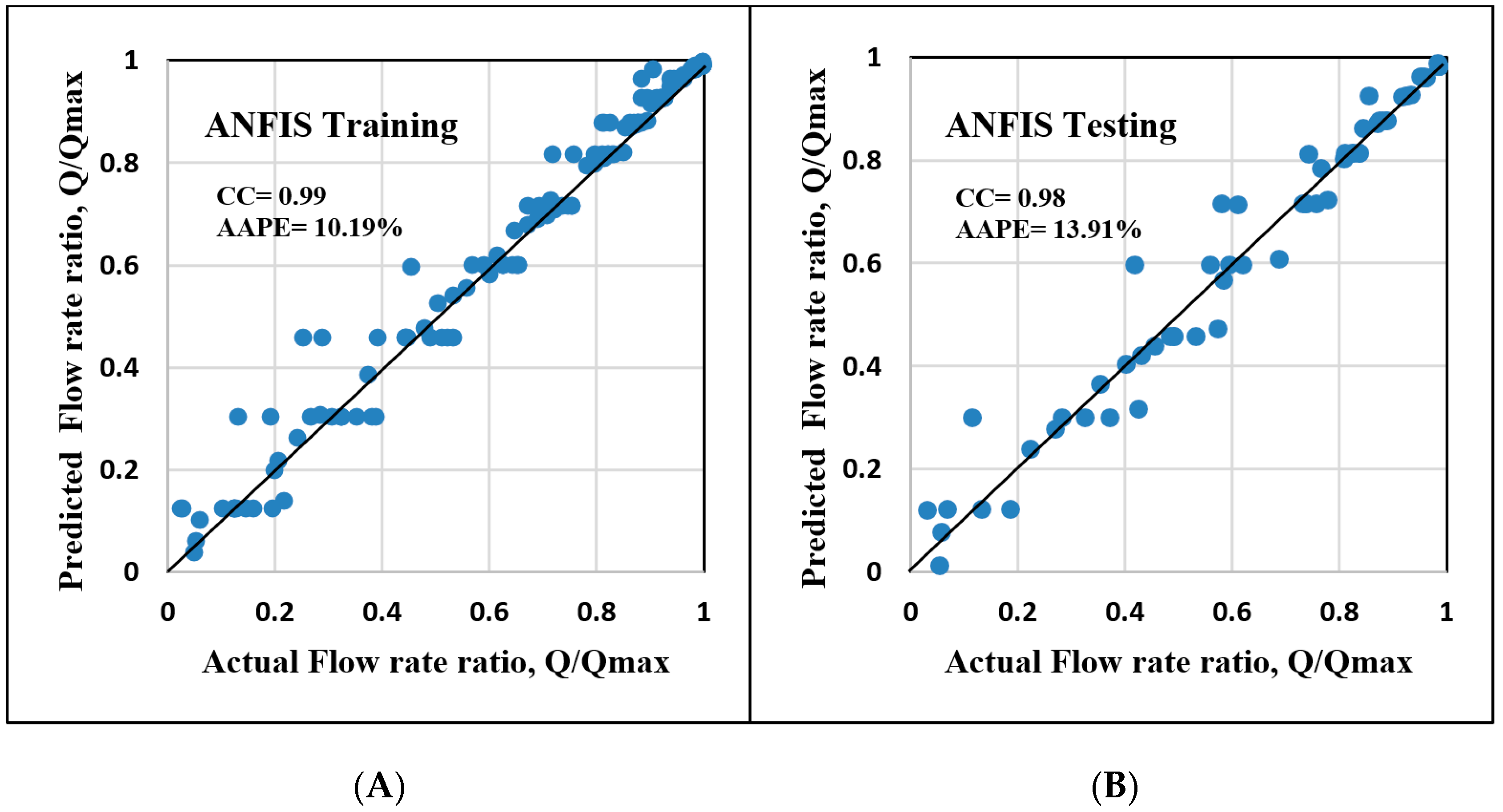
3.2. Fuzzy Logic System
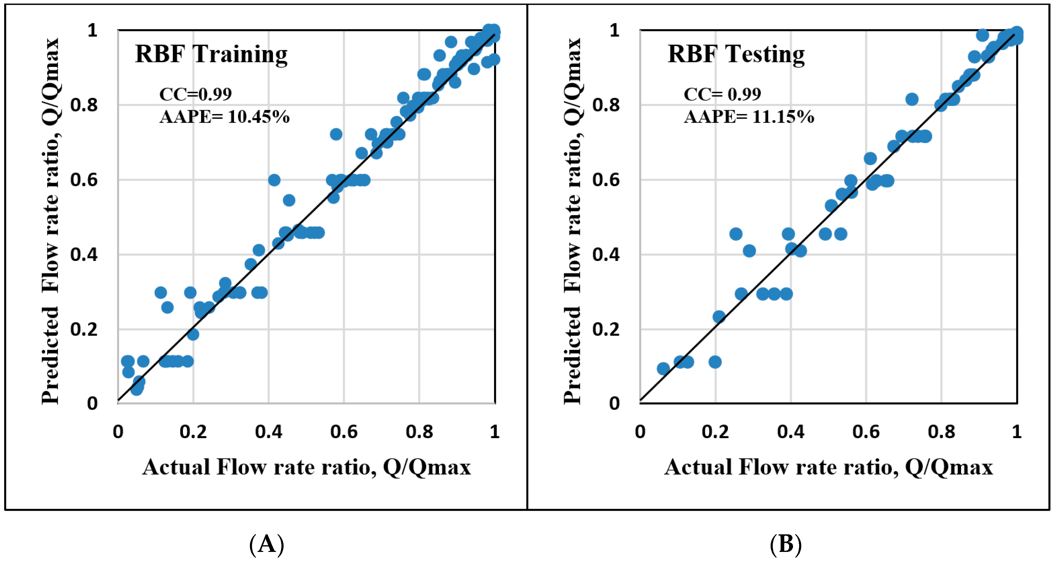
3.3. Radial Basis Function (RBF) Network
3.4. New Empirical Correlation for Fishbone Productivity
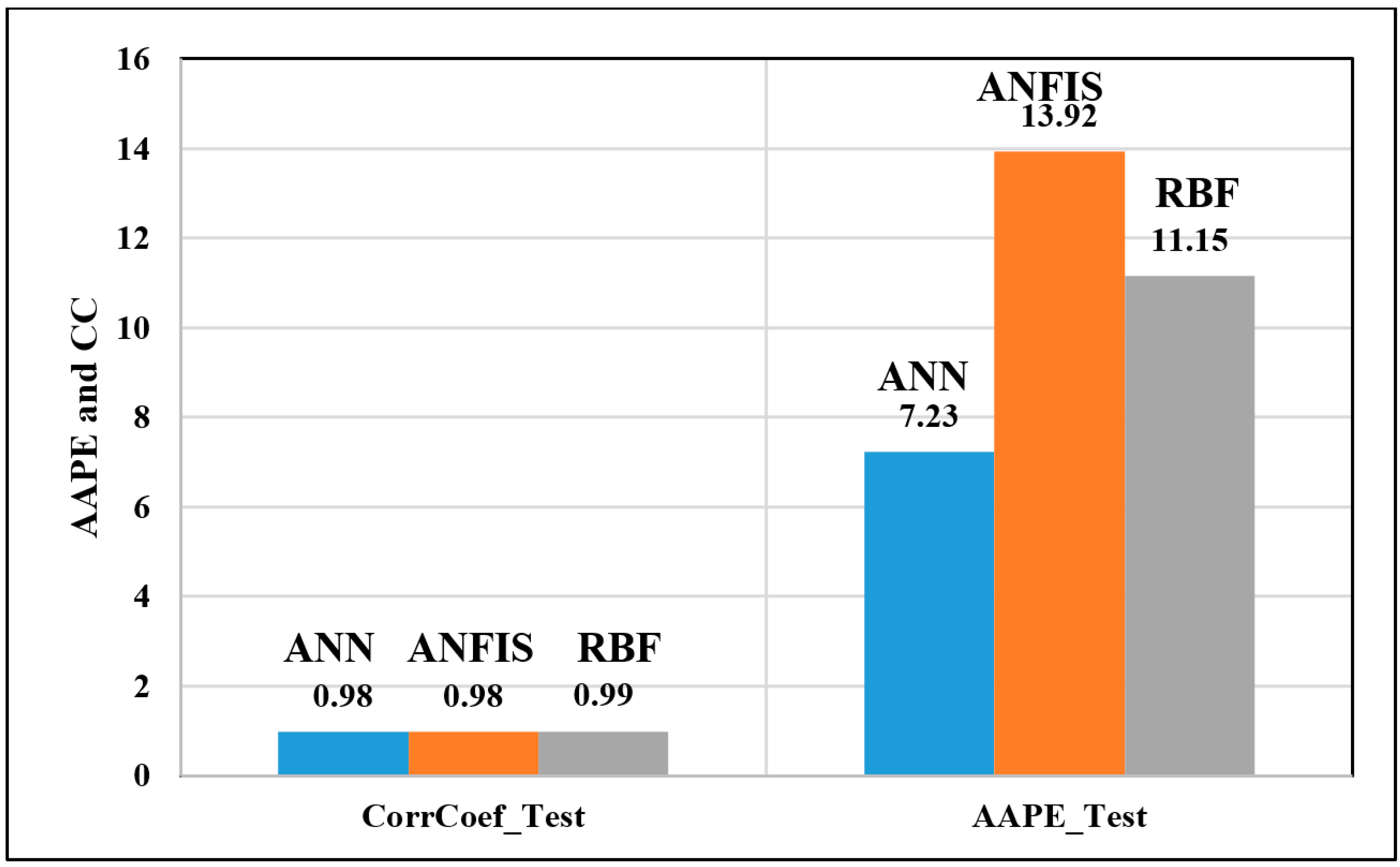
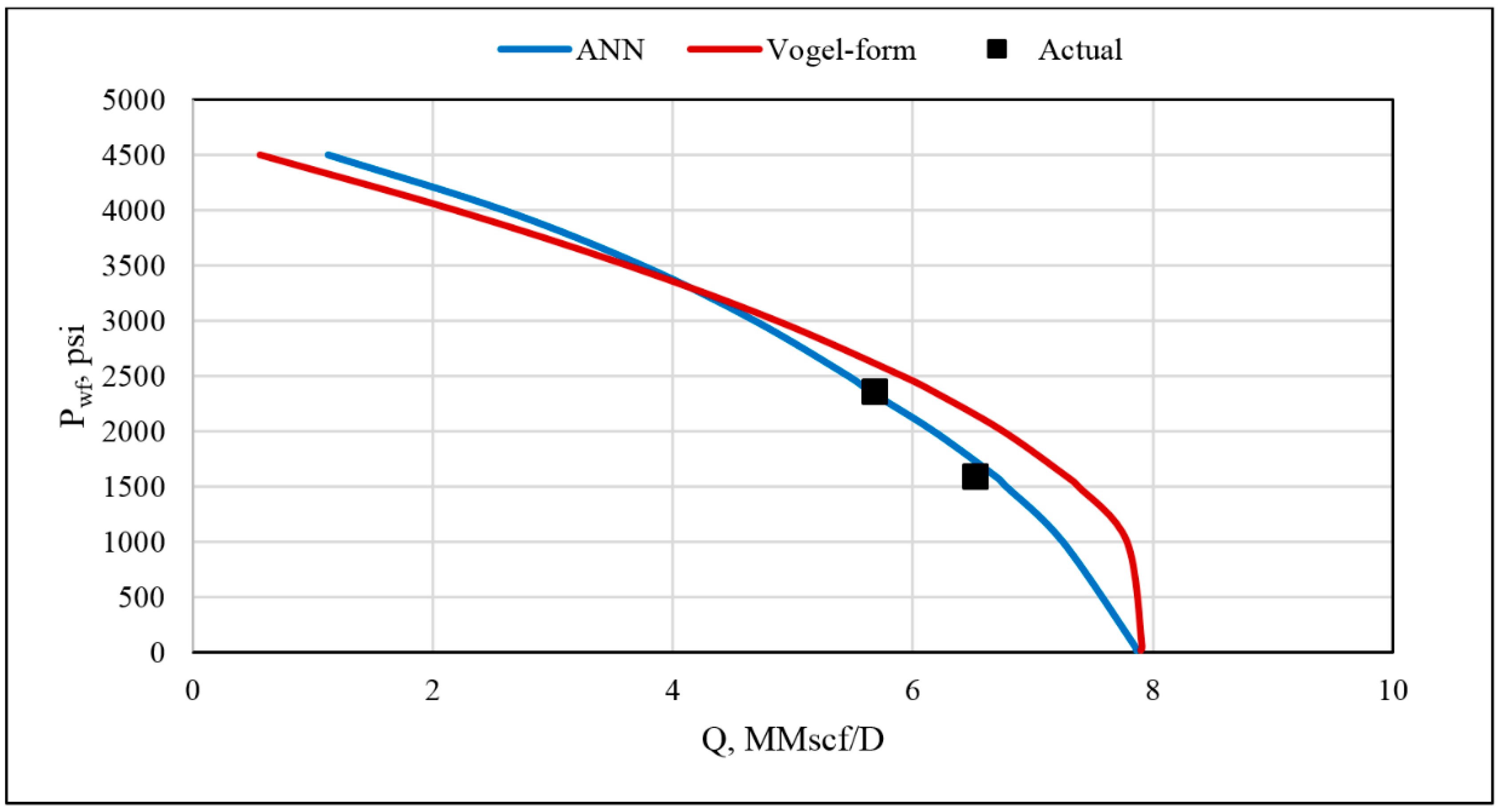
3.5. Model Verification
4. Conclusions
- The developed models showed very acceptable matches between the predicted and actual flow rates for fishbone wells.
- Only three parameters are required as inputs to the models for determining the production rate of fishbone wells: flowing bottomhole pressure, permeability ratio and lateral length.
- The developed models are able to estimate the fishbone productivity without introducing the uncertainty present in numerical models.
- The ANN model outperforms all of the artificial intelligence methods in predicting the fishbone productivity. Absolute errors of 7.23%, 13.92%, and 11.14% were obtained using the neural network, fuzzy logic and radial basis function models, respectively.
- An empirical equation was extracted from the ANN model which can provide a direct and simple determination of fishbone productivity.
- The extracted ANN-based equation can be inserted into commercial production software to provide more accurate predictions for fishbone productivity.
- The proposed models can help production engineers in designing and optimizing their production plans for complex wells.
Author Contributions
Funding
Acknowledgments
Conflicts of Interest
Abbreviations
| AAPE | Average absolute percentage error |
| AAPE_Test | Average absolute percentage error for testing data set |
| ANFIS | Adaptive neuro-fuzzy inference system |
| ANN | Artificial neural network |
| b1 | Bias for hidden layer neuron j |
| b2 | Bias for output layer of ANN model |
| CC | Correlation coefficient |
| CorrCoef_Test | Correlation coefficient for testing data set |
| D | Distance between laterals in ft |
| i | Index for input parameters |
| j | Index for hidden layer neurons |
| Kh | Horizontal permeability in md |
| Kh/Kv | Permeability ratio |
| KV | Vertical permeability in md |
| L | Length of lateral in ft |
| N | Number of lateral or branches |
| Ni | Total number of input parameters |
| Pwf | Flowing bottomhole pressure in psia |
| Pwfmax | Average reservoir pressure in psia. |
| Q | Flow rate in Mscf/D |
| Qmax | Absolute open flow in Mscf/day. |
| w1i | Weights vector between input and hidden layer for ANN model |
| w2i | Weights vector between hidden and output layer for ANN model |
| xi | Input parameters |
References
- Bosworth, X.; El-Sayed, H.S.; Ismail, G.; Ohmer, H.; Stracke, M.; West, C.; Retnanto, A. Key Issues in Multilateral Technology. Oilfield Rew. 1998, 10, 14–28. [Google Scholar]
- Guangyu, X.; Guo, F.; Cheng, S.; Sun, Y.; Yu, J.; Wang, G. Fishbone Well Drilling and Completion Technology in Ultra-Thin Reservoir. In Proceedings of the IADC/SPE Asia Pacific Drilling Technology Conference and Exhibition (Paper IADC/SPE 155958), Tianjin, China, 9–11 July 2012. [Google Scholar]
- Filho, J.C.; Yifei, X.; Sepehrnoori, K. Modeling Fishbones Using the Embedded Discrete Fracture Model Formulation: Sensitivity Analysis and History Matching. In Proceedings of the SPE Annual Technical Conference and Exhibition (SPE-175124-MS), Houston, TX, USA, 28–30 September 2015. [Google Scholar]
- Guo, B.; Sun, K.; Ghalambo, A. Well Productivity Hand Book; Gulf Publishing Company: Houston, TX, USA, 2008; pp. 226–230. [Google Scholar]
- Furui, K.; Zhu, D.; Hill, A.D. A Comprehensive Model of Horizontal Well Completion Performance. In Proceedings of the SPE Annual Technical Conference and Exhibition (Paper SPE 84401), Denver, CO, USA, 5–8 October 2003. [Google Scholar]
- Ahmed, M.E.; Alnuaim, S.; Abdulazeem, A. New Algorithm to Quantify Productivity of Fishbone Type Multilateral Gas Well. In Proceedings of the SPE Annual Technical Conference and Exhibition (SPE-181888-MS), Dubai, UAE, 26–28 September 2016. [Google Scholar]
- Borisov, J.P. Oil Production Using Horizontal and Multiple Deviation Wells; Joshi, S.D., Ed.; Strauss, J., Translator; Phillips Petroleum Co.: Bartlesville, OK, USA, 1984. [Google Scholar]
- Economides, M.J.; Hill, A.D.; Economides, C. Petroleum Production Systems; Prentice Hall PTR: Upper Saddle River, NJ, USA, 1994. [Google Scholar]
- Salas, J.R.; Clifford, P.J.; Jenkins, D.P. Multilateral Well Performance. In Proceedings of the Western Regional Meeting (Paper SPE 35711), Anchorage, AK, USA, 22–24 May 1996. [Google Scholar]
- Yildiz, T. Multilateral Horizontal Well Productivity. In Proceedings of the SPE Europec/EAGE Annual Conference (Paper SPE 94223), Madrid, Spain, 13–16 June 2005. [Google Scholar]
- Xiance, Y.; Guo, B.; Ai, C.; Bu, Z. A comparison between multi-fractured horizontal and fishbone wells for development of low-permeability fields. In Proceedings of the Asia Pacific Oil and Gas Conference and Exhibition (Paper SPE 120579), Jakarta, Indonesia, 4–6 August 2009. [Google Scholar]
- Lian, P.; Cheng, L.; Tan, X.; Li, L. A model for coupling reservoir inflow and wellbore flow in fishbone wells. Pet. Sci. J. 2012, 9, 336–342. [Google Scholar] [CrossRef]
- Ding, Z.; Liu, Y.; Gong, Y.; Xu, N. A new technique: Fishbone well injection. Pet. Sci. Technol. 2012, 30, 2488–2493. [Google Scholar] [CrossRef]
- Freyer, R.; Shaoul, J.R. Laterals stimulation method. In Brasil Offshore Conference and Exhibition; SPE-143381-MS; Society of Petroleum Engineers: Macae, Brazil, 2011. [Google Scholar] [CrossRef]
- Abdulazeem, A.; Alnuaim, S. New Method to Estimate IPR for Fishbone Oil Multilateral Wells in Solution Gas Drive Reservoirs. In Proceedings of the SPE Kingdom of Saudi Arabia Annual Technical Symposium and Exhibition (SPE-182757-MS), Dammam, Saudi Arabia, 25–28 April 2016. [Google Scholar]
- Al-Mashhad, A.S.; Al-Arifi, S.A.; Al-Kadem, M.S.; Al-Dabbous, M.S.; Buhulaigah, A. Multilateral Wells Evaluation Utilizing Artificial Intelligence. In Proceedings of the Abu Dhabi International Petroleum Exhibition and Conference (SPE-183508-MS), Abu Dhabi, UAE, 7–10 November 2016. [Google Scholar]
- McCullock, W.S.; Pitts, W. A logical calculus of the ideas immanent in nervous activity. Bull. Math. Biophys. 1943, 5, 115–133. [Google Scholar] [CrossRef]
- Bailey, D.; Thompson, D. How to Develop Neural Network. AI Expert 1990, 5, 38–47. [Google Scholar]
- Rosenblatt, F. The Perceptron, A Perceiving and Recognizing Automaton; Project Para Report No. 85-460-1; Cornell Aeronautical Laboratory (CAL): Buffalo, NY, USA, 1957. [Google Scholar]
- Fausett, L. Fundamentals of Neural Networks, Architectures, Algorithms, and Applications; Prentice-Hall Inc.: Eaglewood Cliffs, NJ, USA, 1994. [Google Scholar]
- Ali, J.K. Neural Networks: A new Tool for the Petroleum Industry. In Proceedings of the European Petroleum Computer Conference, Aberdeen, UK, 15–17 March 1994. [Google Scholar]
- Russell, S.J.; Norvig, P. Artificial Intelligence: A Modern Approach, 3rd ed.; Prentice Hall: Upper Saddle River, NJ, USA, 2009; ISBN 0-13-604259-7. [Google Scholar]
- Sargolzaei, J.; Saghatoleslami, N.; Mosavi, S.M.; Khoshnoodi, M. Comparative Study of Artificial Neural Networks (ANN) and statistical methods for predicting the performance of Ultrafiltration Process in the Milk Industry. Iran. J. Chem. Eng. 2006, 25, 67–76. [Google Scholar]
- Lippmann, R. An introduction to computing with neural nets. IEEE ASSP Mag. 1987, 4, 4–22. [Google Scholar] [CrossRef]
- Jain, A.K.; Mao, J.; Mohiuddin, K.M. Artificial neural networks: A tutor. Computer 1996, 29, 31–44. [Google Scholar] [CrossRef]
- MathWorks, Inc. Neural Network Toolbox 6, User’s Guide. 2008. Available online: http://128.174.199.77/matlab_pdf/nnet.pdf (accessed on 30 June 2019).
- Tahmasebi, P. A hybrid neural networks-fuzzy logic-genetic algorithm for grade estimation. Comput. Geosci. 2012, 42, 18–27. [Google Scholar] [CrossRef] [PubMed]
- Broomhead, D.S.; David, L. Radial basis functions, multi-variable functional interpolation and adaptive networks. 1988. Available online: https://pdfs.semanticscholar.org/b08b/a914037af6d88d16e2657a65cd9dc5cf5da1.pdf (accessed on 30 June 2019).
- AlAjmi, M.D.; Alarifi, S.A.; Mahsoon, A.H. Improving Multiphase Choke Performance Prediction and Well Production Test Validation Using Artificial Intelligence: A New Milestone. In Proceedings of the SPE Digital Energy Conference and Exhibition (SPE-173394-MS), The Woodlands, TX, USA, 3–5 March 2015. [Google Scholar]
- Alarifi, S.A.; AlNuaim, S.; Abdulraheem, A. Productivity Index Prediction for Oil Horizontal Wells Using Different Artificial Intelligence Techniques. In Proceedings of the SPE Middle East Oil & Gas Show and Conference (SPE-172729-MS), Manama, Bahrain, 8–11 March 2015. [Google Scholar]
- Chen, F.; Duan, Y.; Zhang, J.; Wang, K.; Wang, W. Application of neural network and fuzzy mathematic theory in evaluating the adaptability of inflow control device in horizontal well. J. Pet. Sci. Eng. 2015, 134, 131–142. [Google Scholar]
- Elkatatny, S.; Mahmoud, M.; Tariq, Z.; Abdulraheem, A. New insights into the prediction of heterogeneous carbonate reservoir permeability from well logs using artificial intelligence network. Neural Comput. Appl. 2018, 30, 2673–2683. [Google Scholar] [CrossRef]
- Elkatatny, S.; Tariq, Z.; Mahmoud, M. Real time prediction of drilling fluid rheological properties using Artificial Neural Networks visible mathematical model (white box). J. Pet. Sci. Eng. 2016, 146, 1202–1210. [Google Scholar] [CrossRef]
- Van, S.L.; Chon, B.H. Effective Prediction and Management of a CO2 Flooding Process for Enhancing Oil Recovery using Artificial Neural Networks. ASME J. Energy Resour. Technol. 2018, 140, 032906. [Google Scholar] [CrossRef]
- Van, S.L.; Chon, B.H. Evaluating the critical performances of a CO2–Enhanced oil recovery process using artificial neural network models. J. Pet. Sci. Eng. 2017, 157, 207–222. [Google Scholar] [CrossRef]


| Parameter | Kh/Kv | No. of Laterals | Length (ft) | Distance (ft) | Pwf (psia) | Flow Rate (scf/D) |
|---|---|---|---|---|---|---|
| Minimum | 1 | 2 | 700 | 1300 | 14.7 | 0 |
| Maximum | 1000 | 14 | 3100 | 5200 | 4800 | 197,903.226 |
| Mean | 61 | 6.667 | 2759.523 | 2723.809 | 2359.558 | 81,860.474 |
| Mode | 10 | 6 | 3100 | 2600 | 14.7 | 0 |
| Range | 999 | 12 | 2400 | 3900 | 4785.3 | 197,903.226 |
| Standard Deviation | 211.275 | 2.499 | 693.099 | 685.121 | 1551.738 | 48,712.516 |
| Skewness | 4.192 | 1.412 | −1.9159 | 2.0689 | 0.09535 | −0.118 |
| Kurtosis | 18.73 | 5.358 | 5.3081 | 9.503 | 1.7184 | 2.216 |
| Coefficient of variation | 346.352 | 37.491 | 25.116 | 25.153 | 65.763 | 59.507 |
| Case No. | No. of Hidden Layers | Number of Neurons in Layer | CorrCoef_Test | AAPE_Test |
|---|---|---|---|---|
| 1 | 1 | 10 | 0.9849 | 15.7040 |
| 2 | 1 | 20 | 0.9796 | 7.2327 |
| 3 | 2 | 20 | 0.9547 | 14.4647 |
| 4 | 3 | 20 | 0.9868 | 11.6491 |
| Case No | Cluster Radius | Number of Iterations | CorrCoef_Test | AAPE_Test |
|---|---|---|---|---|
| 1 | 0.1 | 200 | 0.9822 | 14.4962 |
| 2 | 0.3 | 200 | 0.9838 | 14.1589 |
| 3 | 0.8 | 200 | 0.9845 | 13.9187 |
| 4 | 0.7 | 200 | 0.9845 | 13.9242 |
| 5 | 1 | 200 | 0.9845 | 13.9208 |
| 6 | 0.6 | 100 | 0.9848 | 14.0791 |
| Case No. | GOAL | SPREAD | MN, Maximum Number of Neurons | CorrCoef_Test | AAPE_Test |
|---|---|---|---|---|---|
| 1 | 0 | 100 | 10 | 0.8786 | 19.3701 |
| 2 | 0 | 100 | 15 | 0.9830 | 11.4670 |
| 3 | 0 | 100 | 20 | 0.9851 | 11.1697 |
| 4 | 0 | 50 | 20 | 0.9851 | 11.1464 |
| 5 | 0.5 | 10 | 20 | 0.8614 | 32.8188 |
| Neurons (N) | Weights between Input and Hidden Layer (W1) | Weights between Hidden and Output Layer (W2) | Hidden Layer Bias (b1) | Output Layer Bias (b2) | ||
|---|---|---|---|---|---|---|
| Kh/Kv | Length | Pwf | ||||
| 1 | −3.84692 | 0.617902 | −2.26283 | −2.819227146 | 0.752135 | −0.28498 |
| 2 | 3.358502 | −2.56259 | −1.34471 | −2.498195347 | 0.232057 | |
| 3 | 3.162647 | −3.3314 | 1.433747 | −0.682675154 | 0.430348 | |
| 4 | 2.595679 | −3.26074 | −1.83961 | 0.666775968 | −0.9063 | |
| 5 | −2.19077 | 2.3777 | 1.716382 | −2.423948008 | 0.130544 | |
| 6 | −1.74031 | 2.608322 | 2.778165 | −0.581621184 | 0.281862 | |
| 7 | 1.455491 | −2.75341 | −2.49005 | 0.699240526 | −0.74851 | |
| 8 | −1.01596 | 1.755128 | 1.831094 | −2.721731367 | −0.23775 | |
| 9 | −0.51291 | 2.085212 | 1.655426 | −2.701708506 | −0.15973 | |
| 10 | −0.30873 | 3.380575 | −1.66117 | 0.602113511 | 0.173508 | |
| 11 | 0.169321 | −1.10784 | −3.44826 | −1.33129177 | 0.285198 | |
| 12 | −0.35496 | −1.95086 | −2.1071 | 2.340221069 | −0.05304 | |
| 13 | 1.08924 | 2.348532 | 1.9611 | −2.136881713 | 0.191233 | |
| 14 | 1.407857 | 0.420195 | 2.554844 | 2.696650854 | 0.15787 | |
| 15 | −1.74964 | −1.27965 | −0.31507 | 3.224532039 | −0.16893 | |
| 16 | −2.24378 | −1.25899 | 1.524934 | −3.236788256 | −0.11517 | |
| 17 | −2.61158 | −2.64587 | −2.30505 | 1.377837678 | −0.07059 | |
| 18 | 3.316892 | 3.350453 | 0.264872 | −1.109735463 | −0.12635 | |
| 19 | 3.298386 | 1.357587 | −3.4066 | −0.837658734 | 0.641118 | |
| 20 | 3.717023 | 0.598516 | −3.12083 | 1.403728747 | 0.227681 | |
© 2019 by the authors. Licensee MDPI, Basel, Switzerland. This article is an open access article distributed under the terms and conditions of the Creative Commons Attribution (CC BY) license (http://creativecommons.org/licenses/by/4.0/).
Share and Cite
Hassan, A.; Elkatatny, S.; Abdulraheem, A. Application of Artificial Intelligence Techniques to Predict the Well Productivity of Fishbone Wells. Sustainability 2019, 11, 6083. https://doi.org/10.3390/su11216083
Hassan A, Elkatatny S, Abdulraheem A. Application of Artificial Intelligence Techniques to Predict the Well Productivity of Fishbone Wells. Sustainability. 2019; 11(21):6083. https://doi.org/10.3390/su11216083
Chicago/Turabian StyleHassan, Amjed, Salaheldin Elkatatny, and Abdulazeez Abdulraheem. 2019. "Application of Artificial Intelligence Techniques to Predict the Well Productivity of Fishbone Wells" Sustainability 11, no. 21: 6083. https://doi.org/10.3390/su11216083
APA StyleHassan, A., Elkatatny, S., & Abdulraheem, A. (2019). Application of Artificial Intelligence Techniques to Predict the Well Productivity of Fishbone Wells. Sustainability, 11(21), 6083. https://doi.org/10.3390/su11216083