Article

Individual Condensation Trails in Aircraft Trajectory Optimization

Technische Universität Dresden, Institute of Logistics and Aviation, 01069 Dresden, Germany
*
Author to whom correspondence should be addressed.
Sustainability 2019, 11(21), 6082; https://doi.org/10.3390/su11216082
Submission received: 4 October 2019 / Revised: 23 October 2019 / Accepted: 28 October 2019 / Published: 1 November 2019
(This article belongs to the Section Sustainable Transportation)

Abstract

:
Contrails are one of the driving contributors to global warming, induced by aviation. The quantification of the impact of contrails on global warming is nontrivial and requires further in-depth investigation. In detail, condensation trails might even change the algebraic sign between a cooling and a warming effect in an order of magnitude, which is comparable to the impact of aviation-emitted carbon dioxides and nitrogen oxides. This implies the necessity to granularly consider the environmental impact of condensation trails in single-trajectory optimization tools. The intent of this study is the elaboration of all significant factors influencing on the net effect of single condensation trails. Possible simplifications will be proposed for a consideration in single-trajectory optimization tools. Finally, the effects of the most important impact factors, such as latitude, time of the year, and time of the day, wind shear, and atmospheric turbulence as well as their consideration in a multi-criteria trajectory optimization tool are exemplified. The results can be used for an arbitrary trajectory optimization tool with environmental optimization intents.

1. Introduction

The term condensation trail (contrail) summarizes a type of human-induced cloud, developed behind aircraft due to condensation of water vapor emissions and ambient humidity around exhausted soot particles and atmospheric condensation nuclei [1] in a cold ambient atmosphere, satisfying the Schmidt–Appleman criterion [2,3]. In an ice supersaturated environment, these artificial ice clouds form into long-living cirrus clouds called “Cirrus homogenitus” as defined by the World Meteorological Organization [4].
In the Earth–atmosphere energy budget, contrails act like a barrier [5,6,7]. They scatter incoming shortwave solar radiation back to the sky (resulting in a cooling effect) and they absorb and emit the outgoing longwave terrestrial radiation back to the Earth’s surface (yielding a warming effect in the lower layer of the atmosphere) [6,8,9,10]. The dominating effect may be defined as radiative forcing R F , as the change in net downward radiative flux at the tropopause (considering the instantaneous response of the stratosphere) [6]. The contribution of contrails to global warming cannot yet be determined with high precision and depends on flight performance, weather conditions, and time. Latest combinations of several approaches to model a global impact of contrails on global warming summarize a warming net effect of R F Contrail = 0.05 W m 2 with accuracy to within 0.02 and + 0.15 W m 2 for 2010 [6]. Single studies result in a precision of the environmental impact of contrails including negative (cooling) net effects (e.g., R F Contrail = 0.007 to + 0.02 W m 2 for 2005 [9]). Using global climate models and historic air traffic data, reliable estimations of the global contrail radiative forcing for the year 2000 of R F Contrail = 0.03 ( 0.01 to + 0.08 ) W m 2 [9] have been improved for 2010 to R F Contrail = 0.02 ( 0.01 to + 0.03 ) W m 2 [6] considering an increased traffic distance by 22% between 2005 and 2010. For 2002, Burkhardt and Kärcher [10] estimated R F Contrail = 0.03 W m 2 of contrails and contrail cirrus clouds within a global climate model.
Compared to the summed effect of one year’s aviation-emitted carbon dioxide CO 2 and nitrogen oxides NO x which is R F CO 2 , NO x = 0.04 W m 2 [6], the impact of contrails on global warming is no longer negligible [6,11], as it might exceed those effects of CO 2 and NO x , even though contrails are only formed during 10 % of the flights, on a global average [12]. Thus, the need for contrails to be considered in trajectory optimization becomes indisputable.
The impact of single condensation trails on trajectory optimization has been analyzed by Gounou et al. [13] and Forster et al. [14], focusing on the importance of large solar zenith angles during sunset and sunrise. In an application of a Monte Carlo code for photon transport, Forster et al. [14] already considered effects like multiple scattering, but in a coarse spatial grid and ignoring the impact of flight performance on the optical properties of the contrail. Detailed studies on all significant impact factors have been elaborated by Rosenow [11]. In the current study, the results have been simplified and harnessed for trajectory optimization. All other research interests known to the authors concentrated on the effect of contrails on a global scale.
Using satellite data, the adjusted forcing A F as the imbalance of the Earth–atmosphere energy system after stratospheric temperatures have been adjusted to regain a radiative equilibrium in the stratosphere (assuming zero further radiative heating rates) can be calculated [15,16], considering a completed transition of contrails into cirrus. Herewith, the diurnal cycle of contrails and cirrus and differences in regions with low and high air traffic demand can be distinguished [16]. Using satellite data of 2006, A F Contrail = 0.045 to 0.075 W m 2 has been quantified for contrails and contrail-induced cirrus. By applying a combination of modeled and satellite data-based estimates with tolerances in spreading rate, contrails optical depth, ice-particle shape, and radiative transfer [17] and by accounting for the ongoing increase in air traffic, contrails, and contrail-induced cirrus A F Contrail for the year 2010 of A F Contrail = 0.05 ( 0.02 to 0.15 ) W m 2 is widely accepted [6]. Bock and Burkhardt [18] predicted a global future contrail radiative forcing of R F Contrail = 0.159 W m 2 for 2050 assuming R F Contrail = 0.049 W m 2 in 2006 and considering a shift in cruising altitudes, an increase in air traffic distance until 2050 by a factor of 4 compared to 2006, an increase of alternative fuels (with reduced soot emission) and expected changes in propulsion efficiency in 2050. They determined the distribution of the contrail formation taking into account the global distribution of the expected air traffic distance. However, the influence of those contrails on global warming was again determined using global averages. Chen and Gettelman [19] modeled the impact of existing contrails on contrail cirrus ice-crystal shape and size. They predicted an increase in contrail cirrus radiative forcing by a factor of 7 for 2050 (i.e., R F Contrail = 0.087 W m 2 ) compared to 2006 assuming, that air traffic movements will grow on average by a factor of 4 until 2050. In their model, Chen and Gettleman considered a region-specific contrail radiative forcing and a local increase in air traffic. Avila and Sherry [20] estimated the radiative forcing of individual contrails, applying a model developed by Schumann et al. [21], assuming a constant optical depth. Here, contrails are roughly parameterized in terms of optical depth, width, and particle diameter. For each contrail class, an effective particle radius is approximated according to Schumann and each effective radius corresponds to specific optical properties. The large advantage of the study by Avila and Sherry is the consideration of the solar zenith angle.
A consideration of contrails in trajectory optimization tools, if any, has only been found by taking into account a constant value for trajectories through ice-supersaturated regions [22,23,24,25,26]. This consequent avoidance of contrail formation does not, however, lead to a holistically optimized trajectory [27]. Specifically, considering single contrails with a cooling effect on the Earth–atmosphere system is completely misunderstood in those approaches. The rest of the paper is organized as follows: In Section 2, the methodology of each sub-model is presented, whilst in Section 3 the implementation of all sub-models in the trajectory optimization is demonstrated. Furthermore, a validation of the model and a brief discussion of the findings is shown. In Section 4, the findings have been generalized for an easy implementation in a fast-time trajectory optimization tool.

2. Individual Contrails in Trajectory Optimization

The assessment of single contrails in trajectory optimization may be performed in six steps. The procedure is shown in Figure 1.

2.1. Atmosphere GFS Weather Data

First, detailed weather information for the environment around the aspired route is required. Modeled and gridded global forecast data from the Global Forecast System (GFS), provided every six hours in Grib2 format by the National Oceanic and Atmospheric Administration (NOAA) with a spatial resolution of 0.25 degrees at 18 pressure levels is a good compromise between computational effort and accuracy. For trajectory optimization and the estimation of the conditions of contrail formation, vertical profiles of temperature T [K], pressure p [Pa], density ρ [ kg m 3 ], horizontal wind components u [ m s 1 ] and v [ m s 1 ], vertical velocity w [ Pa s 1 ], and the relative humidity r H [-] along the whole route are taken into account.

2.2. Flight Performance

Together with typical input variables for trajectory optimization, such as city pair, aircraft type, engine type, payload, optimization function (i.e., minimum fuel burn, minimum time of flight, minimum contrail impact, or multi-criteria optimization), a trajectory optimization model with implemented key performance assessment can be used for the calculation of the optimum vertical and lateral path. Here, we use the validated simulation environment TOMATO [28,29,30] which includes the aircraft performance model COALA [31,32] for vertical optimization and for the quantification of the emissions. In TOMATO, the trajectory is optimized iteratively by assessing each interim solution regarding several key performance indicators (KPI) including contrails [33]. For comparability, each KPI is transformed into monetary values using the European Emission Scheme. The weighting of the contrail impact in the trajectory optimization is adjusted with prices between €10 and €65 per tonne CO 2 equivalent emission. According to the Institute for Advanced Sustainability Studies, a price of €65 per tonne CO 2 equivalent emission is required to restrict global warming to a limit of d T = 2 °C [34].
For the evaluation of the contrail, two conditions on contrail formation have to be fulfilled: Firstly, the Schmidt–Appleman criterion [2,3] determines the threshold temperature T LC of the atmosphere which is required to overcome the exhaust heat. T LC depends on the aircraft true air speed v TAS [ m s 1 ], thrust F [N], fuel flow m ˙ f [ kg s 1 ], specific combustion heat of kerosene Q = 43 MJ kg 1 , and on the emission index of water vapor E I water = 1.24 kg 1 [11]. The mixing of the exhaust emissions with the ambient atmosphere follows a straight line in an enthalpy-mass diagram with the slope G
G = Q ( 1 η ) E I water ,
where η defines the overall propulsion efficiency as the fraction between resulting energy (thrust F and true air speed v TAS ) and required energy (specific combustion heat Q and fuel flow m ˙ f )
η = F v TAS Q m ˙ f .
In case of the mixing line of the exhaust emissions with the ambient atmosphere touching the saturation water vapor pressure, contrail formation takes place (see [2,3,11] for more details). From this, it follows that the larger the G the higher the threshold temperature for contrail formation and the higher the probability of contrail formation. The second criteria for contrail formation is an ice-supersaturation of the ambient atmosphere in order to survive the vortex regime of the wake vortices, wherein the exhaust emissions are captured [35,36]. Therewith, sufficient humidity for a constant ice-particle growth is provided. Each criteria, the Schmidt–Appleman criterion and the ice-supersaturation, is examined for each second of the flight performance calculation.

2.3. Contrail Life Cycle

In the case of both criteria, the Schmidt–Appleman criterion and the ice-supersaturation, being satisfied, T, p, ρ , u, v, w, r H , longitude l o n [°], latitude l a t [°], altitude z [m], m ˙ f [ kg s 1 ], and time t [s] are provided by COALA to the “Contrail Life Cycle” model [11,37] for each time step, a contrail is induced. For the initial dimensions, a wake vortex model [38] is applied and calibrated for each aircraft type, implemented in COALA. The initial decay of the contrail in the vortex regime strongly depends on atmospheric turbulence (see Figure 2, right), which is approximated by the energy dissipation rate ε [ m 2 s 3 ] as conversion of kinetic energy due to molecular friction per unit mass and per time into thermal energy [39]. ε is calculated assuming a lognormal distribution of turbulence in the lower troposphere and upper stratosphere and a linear correlation between a logarithmic diagnostic turbulence value, such as the vertical velocity w [Pa s 1 ], provided by the GFS [40,41]. The vertical velocity w is defined as the Lagrangian rate of change of pressure with time [42]
w = d p d t .
Furthermore, wind shear s h [s 1 ] (Figure 2, left) as difference in wind velocity u and v [ m s 1 ] between two altitudes Δ z [m] strongly influences the 2D sheared Gaussian plume model for contrail dispersion [11,37]. Δ z is called shear layer and depends on the maximum differences in wind velocity between two altitudes. s h is also calculated from the provided weather data. The sheared diffusivity D s [m 2 s 1 ] is assumed to be in the range of the square root of the vertical D v [m 2 s 1 ] and horizontal diffusivity D h [m 2 s 1 ]: D s D v D h [43], but D s D v D h [11]. Assuming a soot emission index of E I soot = 0.04 g kg 1 kerosene [44] and a proportional share of ice-particles in the contrail [44], all variables impacting the optical properties of the contrail can be provided to the “Contrail Life Cycle” model. In fact, these are the horizontal σ ^ h ( t ) [ m 2 ], vertical σ ^ v ( t ) [ m 2 ], and sheared σ ^ s ( t ) [ m 2 ] components of the contrail diffusivity variance σ ^ ( t ) [ m 2 ], the contrail cross section C C S ( t ) [m 2 ], the ice-water content I W C ( t ) [ kg m 3 ] as total amount of ice mass per volume contrail, the number of ice-particles n p (hereafter called ice-particle number density) [ m 3 ] and the projected particle area A p [m 2 ]. The impact of s h , ε , and vertical wind speed v z [ m s 1 ] on the particle radius and the contrail lifetime is shown in Figure 2 and Figure 3, respectively. The vertical wind speed v z can be calculated from the mean divergence of the horizontal wind speed, averaged along the vertical axis between ground and flight level [45]. Furthermore, v z can be calculated from vertical velocity w using
v z = w ρ g
where ρ [kg m 3 ] denotes the ambient air density and g [m s 2 ] the gravitational acceleration. Thereby, negative values indicate upward wind speeds. On average, values of v z ¯ = 0.005 m s 1 are calculated. The vertical wind velocity is two orders of magnitudes smaller than the horizontal wind velocity and a vertical upwind velocity of v z = 0.005 m s 1 is realistic in stable stratification [46]. Assuming this vertical upward speed and a sedimentation of the ice-particles following Stoke’s law, the contrail sediments as soon as the ice-particle radius exceeds values of r p 6 μ m [11].
Note, the available ice-water content is distributed equally to the available number of ice-particles per contrail volume. During cruise, aircraft fly with a speed between maximum Mach number (upper boundary) and a maximum specific range (lower boundary). Within this range, fuel flow decreases with decreasing speed. Since the number of emitted soot particles is assumed to be proportional to the fuel flow, a decreasing fuel flow (as a consequence of a decreasing speed) causes a lower number of soot particles (as primary condensation nuclei). The water vapor in the atmosphere and from the emissions thus sublimates to a lower number of soot particles. As a result, fewer but larger ice-particles are formed. However, the optical properties of contrails depend more strongly on ice-particle size than on ice-particle number density [11]. From this follows that flying slowly through ice-supersaturated regions causes more radiative effective contrails. Furthermore, according to the Schmidt–Appleman criterion [2,3], the higher the overall engine efficiency, the lower the exhaust gas temperature, the higher the critical atmospheric temperature ( T LC ) for contrail formation [47]. The critical atmospheric temperature for contrail formation T LC positively correlates with thrust, true air speed v TAS , and fuel flow m ˙ f . The higher the T LC , the higher the probability of contrail formation in an ice- supersaturated region. In general, optimized air speeds for highly efficient conditions of combustion (i.e., minimum fuel flow) refer to low values of T A S . Both facts support the thesis that cold, ice-supersaturated regions should preferably be flown through with high speeds.

2.4. Contrail Optical Properties

The fourth step is the “Contrail Optical Properties” model. Depending on the geometrical and microphysical properties of the contrail, the radiative extinction due to scattering, absorption, and emission within the contrail is calculated by running a Monte Carlo Simulation to consider multiple scattering events which are likely, especially for large solar zenith angles θ [rad] [11]. Therefore, Beer’s law
I λ ( s 1 ) I λ ( s 2 ) = exp s 1 s 2 Q e A p n p ( s ) d s
is used, where I λ ( s 2 ) and I λ ( s 1 ) denote the original and the extinguished wavelength specific radiation of solar intensities [ W m 2 sr 1 ] and of terrestrial irradiances [ W m 2 ] (see Figure 4). Q e ( s ) denotes the extinction efficiency [-] and depends on wavelength, particle size, and shape [11,48] and A p denotes the projected particle area [m 2 ]. Q e ( s ) and A p (s) are not constant within the contrail and depend on the position s. In the “Contrail Optical Properties” model, I λ ( s 1 ) I λ ( s 2 ) Equation (5) is interpreted as a number ratio of extinguished photons, regardless of the amount of radiation irradiating the contrail (see Figure 4) [11,49].
The extinction of photons is calculated for each direction in space individually, considering ice-particle shape-dependent and wavelength-dependent probability of an extinguishing event. The latter is described by the absorption and scattering efficiency Q a ( s ) , Q s ( s ) . Q s ( s ) + Q a ( s ) = Q e ( s ) are parameterized by Wyser et al. [48] and Yang et al. [50] as functions of wavelength, ice-particle size, shape, and density, which in turn are provided by the Gaussian plume model (see Figure 4).
This “Contrail Optical Properties” model provides weighted number ratios S i ( λ , d ω ) of extinguished photons per meter contrail, per wavelength and per time step of the contrail life cycle (Figure 4). For each direction of incoming photons, S i ( λ , d ω ) [m] is calculated by
S i ( λ , t , d ω ) = N out N in w in sin α ,
where N out and N in = 10 7 denote the number of outgoing and incoming photons, respectively. w in = 6 σ ^ h ( t ) denotes the irradiated width of the contrail, α defines the angle between the length axis of the contrail and the incoming photons (see Figure 5). This extinction strongly depends on the direction of irradiation (i.e., α ). The longer the travel distance of photons through the contrail (i.e., the larger α ), the higher the probability that an extinguishing event takes place. With increasing travel distance and with increasing α , the number of out-scattered photons increases, although a dominating forward scattering is expected [48,50,51]. From this follows that during horizontal photon transport during sunrise and sunset, more photons will be scattered in the opposite hemisphere compared to a vertical photon transport at noon. However, the contrail radiative extinction further depends on the power with which the contrail is irradiated, which will be maximum at noon and minimum at night. This power is calculated separately in the next step.

2.5. Atmospheric Radiative Transfer

The fifth step of the approach provides wavelength and angular specific solar intensities and terrestrial irradiances at the position of the contrail. This step is necessary, because the radiative extinction due to the contrail does not only depend on the optical properties of the contrail itself but also on the amount of radiation irradiating the contrail. The powers of solar intensities and terrestrial irradiances depend on wavelength, longitude, latitude, altitude, the presence of clouds, time of the day, and time of the year. Most of these input variables are provided by the flight performance model (see Figure 1). For the calculation of this “Atmospheric Radiative Transfer”, the radiative transfer software package libRadtran [52] is used. Due to different properties of solar and terrestrial extinction in the atmosphere, different radiative transfer solvers are used.

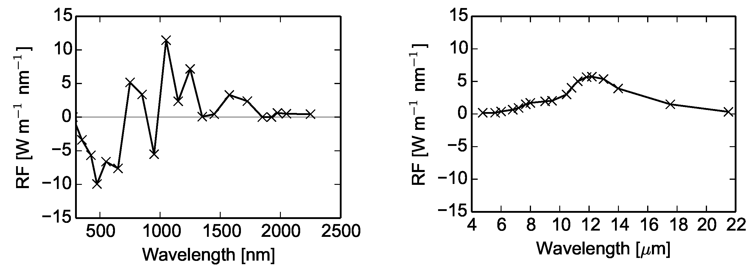
2.5.1. Terrestrial Radiative Transfer

In the terrestrial wavelength spectrum ( 3 λ 100 μ m ), absorption by atmospheric molecules strongly depends on wavelength and varies between neighboring wavelengths. These narrow absorption bands require a high spectral resolution in the radiative transfer calculation and therefore a high computational effort. However, a weak angular dependence (described by zenith angle θ and azimuthal angle ϕ ) of radiation due to a missing part of direct irradiance is expected. The two stream approximation (TSA) takes advantage of the weak angular dependence and reduces the computational effort [53]. Here, all shares of radiation coming from one hemisphere are azimuthally averaged over the half-space and are treated as a single irradiance F [ W m 2 ] without specific information conserning the angular direction (see Figure 6, left). Due to this average, two irradiances at any altitude remain: terrestrial irradiances coming from the lower hemisphere
F up ( λ , t , θ = 1 / 2 π . . . 3 / 2 π )
and terrestrial irradiances coming from the upper hemisphere
F down ( λ , t , θ = 3 / 2 π . . . 1 / 2 π )
(see Figure 6, left) [11].

2.5.2. Solar Radiative Transfer

In the solar wavelength spectrum ( 0 λ 4 μ m , see Figure 7) a TSA is out of the question because of a large influence of the direct beam (in the direction of the position of the sun) on the radiation field. This influence causes a strong angular radiative dependence which cannot be described by a TSA. The radiative transfer solver DISORT (DIScrete Ordinate Radiative Transfer solver) is used for the angular-dependent calculation of direct solar intensities [ mW sr 1 m 2 nm 1 ].
I dir ( λ , t , lon , lat , Ω )
Here, the direction of the direct beam, Ω [sr], is described by the solar zenith angle and the solar azimuthal angle. Diffuse solar intensities (Equation (10)) [ mW sr 1 m 2 nm 1 ]
I diff ( λ , t , lon , lat , θ , ϕ )
depending on longitude, latitude, altitude, time of the day, and time of the year [54] are also provided by DISORT. DISORT is the most used, recommended and most updated solver for angular-depending radiative transfer in the shortwave spectrum [11,55]. Diffuse solar intensities I diff are calculated with an angular discretization of d θ = d ϕ = 2 and the direct beam I dir is added to the solid angle d ω [sr]
d ω = sin θ d θ d ϕ ,
where θ and ϕ , are the solar zenith and azimuthal angle, respectively (see Figure 6, right) [11]. Figure 7 clearly indicates the different contributions of wavelength-specific irradiances on the radiation budget of the earth–atmosphere system. Hence, a consideration of solar irradiances around the maximum at λ = 0.55 (i.e., 0.2 < λ < 1 μ m) would be sufficient. Terrestrial irradiances should be considered between 5 < λ < 22 μ m. Additionally, Figure 7 proves the significant impact of atmospheric absorption by comparing the modeled irradiances with the theoretical values, calculated with Planck’s function assuming mean temperatures of 5750 K of the sun and 288 K of the Earth’s surface.

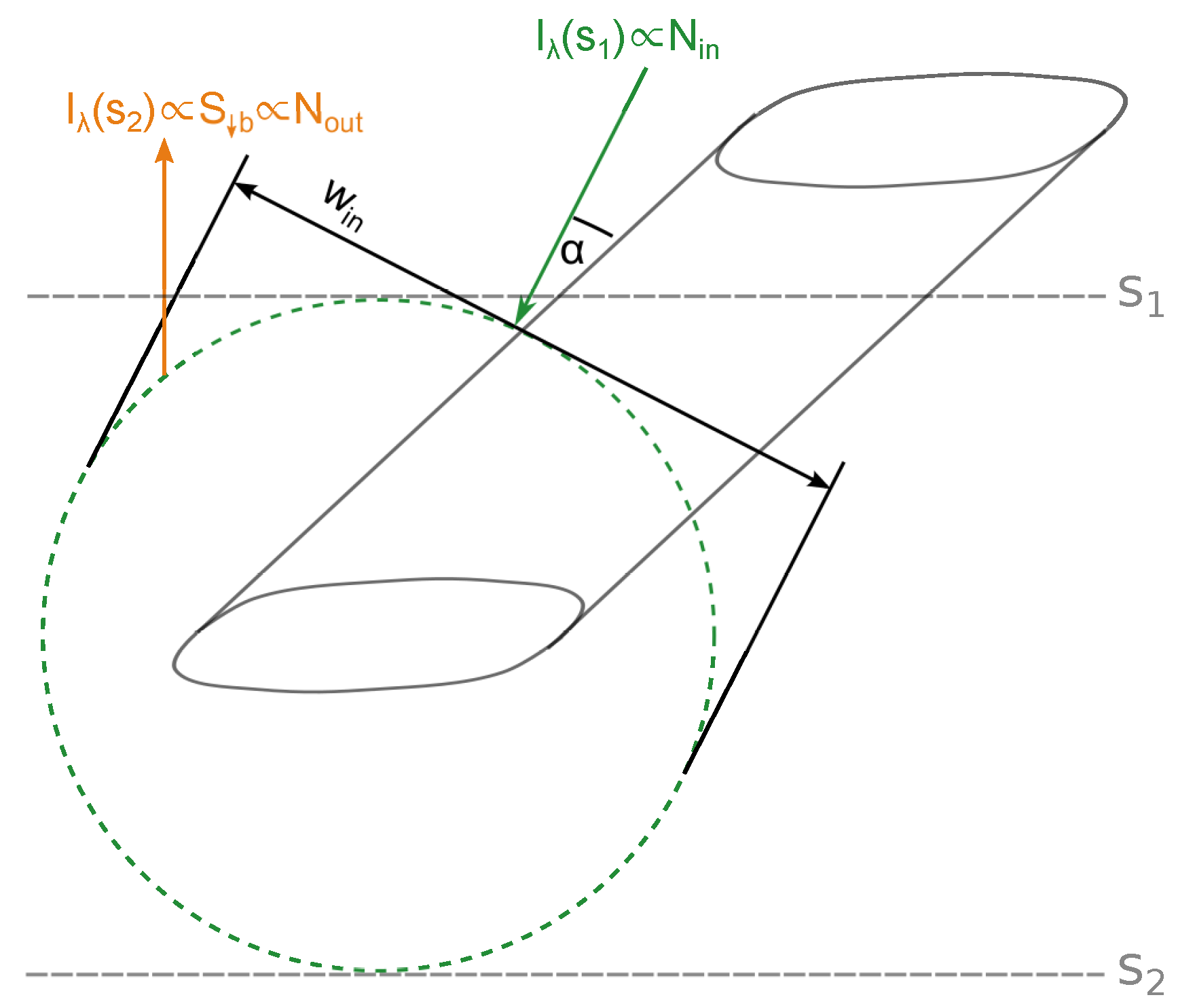
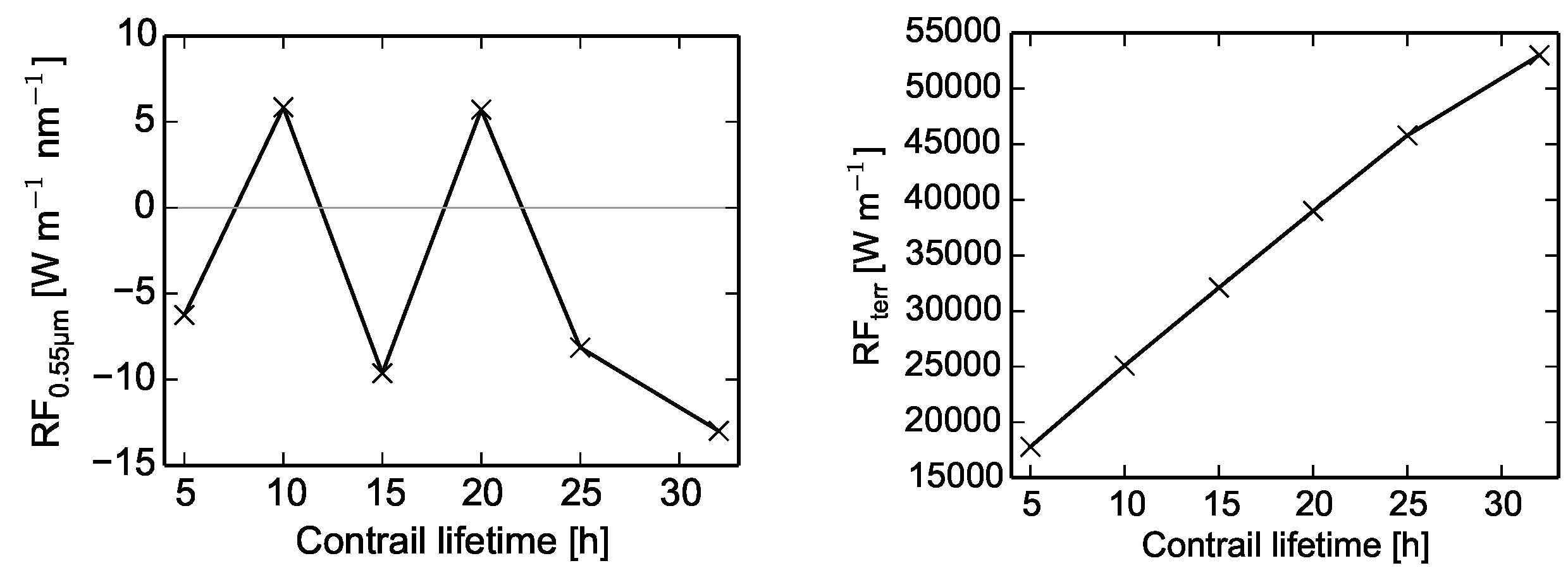
2.6. Contrail Radiative Forcing

The radiative quantities of the “Atmospheric Radiative Transfer” model are multiplied with the extinguished number ratios, provided by the “Contrail Optical Properties” model to estimate the wavelength-specific and direction-specific extinction of radiation due to the contrail. Because the contrail radiative forcing is defined as imbalance of the radiation budget at a horizontal layer, we distinguish between sources and drains of radiation in the upper and in the lower hemisphere of the contrail (see Figure 8).
To calculate the radiative forcing per unit length of the contrail, the power P i ( λ , t , lon , lat , d ω ) [ W m 1 nm 1 ] of the extinguished photons once irradiated on a unit length contrail have to be considered and balanced. Therefore, the solar intensities in Equation (10) and the terrestrial irradiances in Equations (7) and (8) coming from a particular solid angle d ω [sr], (calculated by the “Atmospheric Radiative Transfer” model) have to be weighted by the weighted number ratios of extinguished photons S i [m] (Equation (6)) (from the “Contrail Optical Properties” model) and the corresponding solid angle d ω i . Therefore, only the backscattered and absorbed powers are of interest and the extinguished powers can be summarized to the following components (see Figure 8):
  • P a : number of absorbed photons coming from below;
  • P b : number of photons coming from below, scattered into the lower hemisphere;
  • P b : number of photons coming from above, scattered into the upper hemisphere.
For radiation coming from a particular solid angle d ω i (Equation (11)) and getting scattered into the same hemisphere (i.e., backscattered), the extinguished power P b ( λ , t , lon , lat , d ω i ) [ W m 1 nm 1 ] is
P b ( λ , t , d ω i ) = I ( λ , t , d ω i ) · S b ( λ , t , d ω i ) · d ω i P b ( λ , t , d ω i ) = I ( λ , t , d ω i ) · S b ( λ , t , d ω i ) · d ω i P a ( λ , t , d ω i ) = I ( λ , t , d ω i ) · S a ( λ , t , d ω i ) · d ω i ,
where S b ( λ , t , d ω i ) denotes the weighted number ratio of backscattered photons coming from a particular solid angle d ω i and getting scattered into the same hemisphere and I ( λ , t , d ω i ) is the wavelength-specific solar intensity from the particular solid angle d ω i . In the same way, absorbed solar powers P a ( λ , t , lon , lat , d ω i ) are calculated for each wavelength λ and each solid angle d ω i .
Terrestrial irradiances F up and F down [ W m 2 nm 1 ], calculated with the two stream approximation, are hemispherically averaged irradiances. To estimate the extinguished power in the terrestrial wavelength spectrum, F up and F down have to be weighted by the number ratio of extinguished photons coming from the upper hemisphere S b and the lower hemisphere S b with both getting scattered into the same hemisphere that they are coming from and the absorbed photons coming from all directions S a . For example:
P b ( λ , t ) = F down S b ( λ , t )
P b ( λ , t ) = F up S b ( λ , t )
P a ( λ , t ) = F down ( λ , t ) S a ( λ , t )
+ F up ( λ , t ) S a ( λ , t ) .
The backscattered powers P b , ( λ , t , lon , lat , d ω ) are categorized into two classes: Firstly, backscattered powers from the upper hemisphere P b ( θ = 3 2 π . . . 1 2 π ) (resulting in a cooling effect) and secondly, backscattered powers from the lower hemisphere P b ( θ = 1 2 π . . . 3 2 π ) (with a heating effect, see Figure 8). Absorbed powers P a ( λ , t , lon , lat , d ω ) coming from both hemispheres always contribute to a contrail heating. Those components contribute to the radiative forcing R F Contrail
R F Contrail , m = P a P b + P b .
After integrating over all significant wavelengths, time steps of the contrail life cycle and over the contrail length, each with different optical properties S i ( λ , t ) , the total radiative forcing R F Contrail , m [W m 1 ] (Equation (16)) per meter of an individual contrail can be estimated. Multiplying Equation (16) with the length L Contrail of the contrail with similar optical properties offers the extinguished power [W] due to the contrail. Usually, the radiative forcing is related to the Earth’s surface, which is A Earth = 5.1 × 10 14 m 2 . Hence, the estimated extinguished power is divided by A Earth .
R F Contrail = R F Contrail , m L Contrail A Earth .

2.7. Weighting of Contrail Costs in Trajectory Optimization

The integration of R F Contrail over the whole life cycle, over all significant wavelengths and the division by A Earth offers a comparison with the impact of a reference emission (e.g., CO 2 ) over the whole flight.
Usually, a certain time horizon H (e.g., H = 100 years) is considered in these interpretations. In this case, the ratio of R F Contrail over R F CO 2 (known as the global warming potential, G W P )
G W P = 0 H R F Contrail ( t ) d t 0 H R F CO 2 ( t ) d t ,
is used to calculate CO 2 equivalent emissions, which are transferred into monetary values by applying political instruments, such as the emission trading scheme (ETS). For instance, for H = 100 years, the radiative forcing of the total amount of CO 2 in the atmosphere is [56]
0 H = 100 R F CO 2 ( t ) d t = α CO 2 ln C C 0 = 1.94 W m 2 ,
where α CO 2 = 5.35 denotes a constant [56], C = 399.39 ppm is the actual concentration of CO 2 [57], and C 0 = 278 ppm is the pre-industrial concentration of CO 2 in 1959 [57].
Equation (19) considers the total sum of CO 2 emissions in 100 years and is not restricted to the aviation-transport sector. The radiative impact of CO 2 strongly depends on the altitude of emission. In high altitudes (above the tropopause with low vertical exchange), CO 2 exists for 400 years. In low altitudes (below the tropopause) precipitation induces washing-off effects of CO 2 . Those large differences in the residence time complicate the use of Equation (19) for a comparison of aviation-induced radiative forcing due to contrails and CO 2 emissions.
However, from the literature review in the introduction of this paper, we know the amount of CO 2 emissions caused by aviation in 2005
m CO 2 , 2005 = 733 × 10 6 t a 1 ,
Ref. [7] and the radiative forcing of those emissions
R F CO 2 , 2005 = 0.028 W m 2 .
Hence, the impact of each tonne CO 2 emitted by aviation in 2005 was
R F CO 2 = 3.8 × 10 11 W m 2 t CO 2 1 .
Therewith, the radiative forcing of an individual contrail, calculated in Equation (17), can be transformed into tonnes of CO 2 equivalent emissions, which can be used as external costs in a multi-criteria trajectory optimization.
m CO 2 eq = R F Contrail 3 . 8 × 10 11 W m 2 t CO 2 1 .
By weighting the price per tonne of CO 2 equivalent emission, contrails are considered in the multi-criteria trajectory optimization TOMATO. Following global approximations, as elaborated in the introduction, it is expected that the radiative impact of a single flight’s contrail exceeds those effects of CO 2 .

3. Results

3.1. Contrails in Trajectory Optimization

The most important effects of R F Contrail are determined by the angle α between the length axis of the contrail and the incoming photons (see Figure 4), because it determines the travel distance of photons through the contrail. Furthermore, R F Contrail depends on the order of magnitude of incoming radiation, depending on wavelength (solar > terrestrial), time of the day and year (summer, noon > winter, morning, and evening) and on latitude (equator > pole). Both effects are shown in Figure 9, because α and solar intensity change with daytime. Although the amount of backscattered power P b dominates over the whole day, the sum of downward backscattered power P b and absorbed power P a nearly compensates P b between 7 a.m. and 5 p.m. Only during sunrise and sunset with horizontal photon transport (around 6 a.m. and 6 p.m.), is R F Contrail significantly negative. The closer the contrail is to a pole (high latitudes), the longer the horizontal photon transport takes place. This is why, the ”sunrise–sunset effect” increases with increasing latitude, but the amount of incoming radiation (i.e., the amplitude in Figure 9 decreases with increasing latitude).
Although in Figure 9 the extinguished powers of only a single wavelength are shown, the statement of the results may be transferred to the narrow wavelength band around 0.2 < λ < 2 μ m. In Figure 10, simulations of the whole solar spectrum with significant contribution to the energy budget with wavelengths between 0.55 μ m λ 4.5 μ m (left) and of the most important terrestrial spectrum wavelengths between 4.5 μ m λ 21.5 μ m (right) are shown. Figure 10, left, indicates a decreasing solar effect with increasing wavelength due to a decreasing solar intensity and an increasing share of absorbed power. However, with increasing wavelength, positive values of R F contrail become more dominant. Note, in Figure 9 and Figure 10, only the radiative properties of a single contrail with specific optical properties are calculated. The absorption efficiency Q a , known as the possibility of an absorbing event within the contrail, strongly varies with ice-particle size and shape, which is why the fluctuation in Figure 10, left, is very contrail-specific.
The strong impact of ice-particle size on Q a causes an increasing terrestrial radiative forcing with increasing contrail lifetime (see Figure 2, Figure 3, and Figure 11, for increasing ice-particle radius with lifetime). Additionally, an increasing contrail width with lifetime causes a more distinct radiative forcing of older contrails. Note, the solar radiative forcing (Figure 11, left) is shown only for a single wavelength λ = 0.55 μ m , whereas the terrestrial R F Contrail is integrated over the whole significant terrestrial spectrum 4.5 μ m λ 21.5 μ m . However, at λ = 0.55 μ m the solar intensities are maximum (see Figure 7). Hence, the main solar contribution to R F Contrail is covered. Furthermore, the optical properties depending on shape, size, and number density of ice crystals and on wavelength are only parameterized for discrete wavelengths at 0.55 μ m , 1.35 μ m , 2.25 μ m , 2.75 μ m , 3.0125 μ m , 3.775 μ m , and 4.5 μ m [48]. These wavelengths are used as sampling points in the integration over the whole solar wavelength spectrum. these calculations have not to been carried out as functions of particle shape and size. That is why the solar radiative forcing (Figure 11, left) is only shown for a single wavelength. More detailed results are shown in [11].
Finally, the impact of the consideration of contrails in trajectory optimization is exemplified in Figure 12. Here, blue squares denote ice-supersaturated regions wherein contrail formation is very likely. For this example flight from Los Angeles (LAX) to Boston (BOS), different routes are calculated and compared with each other. The originally filed route (black, 4580 km ground distance) induced a contrail with a length of L Contrail = 1705 km ground distance. The mean optical properties of this contrail have been estimated to R F Contrail = 0.305 W m 1 which is 10.19 × 10 9 W m 2 using Equation (17). Following Equation (23), this contrail must be weighted with 26.81 t CO 2 equivalent emissions. If this value is divided by the total length of the contrail ( L Contrail = 1705 km), we obtain an average amount of 0.0157 t CO 2 km 1 equivalent emissions per km contrail. Considering 0.0157 t CO 2 km 1 and €65 per tonne CO 2 equivalent emission in a multi-criteria trajectory optimization, the contrail would have been completely avoided (red route in Figure 12 with 4730 km ground distance). A more harmonized trajectory with a reduced contrail length of L Contrail = 1374 km ground distance constitutes the green route in Figure 12 with a total ground distance of 4246 km and a contrail weighting of 0.0125 t CO 2 km 1 .

3.2. Verification

To verify the contrail radiative forcing model, a comparison with the results of other publications is carried out whenever possible. Mostly, the optical thickness τ is used to describe the optical properties of a single contrail, measured vertically through the atmosphere. In the present study, the contrail is treated as a Gaussian plume without defined boundaries, but the optical thickness τ strongly depends on the contrail irradiated width. The larger the irradiated width, the smaller the optical thickness at constant irradiation, because the share of photons traveling through the contrail core is reduced. Furthermore, measurements of contrail optical properties are error-prone because of difficult measuring conditions at cruising altitude, where the contrail is hardly visible. For measuring the optical contrail properties, the shape, size, and number density of ice crystals have to be estimated. Therefore, the ice crystals must be captured and examined. Due to high aircraft speeds (≈ 220 m s 1 ), the crystals shatter when caught [58]. From this follows that only a few studies remain for a model verification. For example, Forster et al. [14] and Gounou et al. [13] published the corresponding contrail width to the optical thickness. This width can be interpreted as the irradiated width used in the present radiative forcing model. Hence, the weighted number ratios of extinguished to evaluated photons S ext , which is the sum of S a , S b , and S f multiplied with the irradiated width, can be used for comparison with other publications. In Table 1, values of the weighted number ratios S ext of a non-sheared contrail in a mid-latitude summer atmosphere for several contrail ages derived by Forster et al. [14] are compared with the present weighted number ratios S ext at λ = 0.55 μ m . Although different atmosphere conditions are used by Forster et al., and despite the fact that Forster et al. integrated the radiative extinction over the whole solar and terrestrial spectrum, the results of the weighted number ratios are in the same order of magnitude.
The influence of the solar zenith angle on radiative extinction can be compared with Gounou et al. [13] as well as with Forster et al. [14]. Gounou et al. [13] published the radiative forcing R F [ W m 2 ] of a dense blanket of contrails, integrated over the whole spectrum. Nevertheless, the shape of the extinction depending on solar zenith angle should be similar to the results observed in the present study. Figure 13 shows the typical minimum of radiative forcing at solar zenith angles around θ 70 ° as observed by Gounou et al. [13] and Forster et al. [14].

3.3. Discussion

In this study, a method is described to consider the environmental impact of individual condensation trails in a multi-criteria trajectory optimization. Thereby, three research questions have been answered:
  • How can the conditions of contrail formation be estimated in a flight performance model?
  • What is the radiative impact of the induced contrail per flight time step?
  • How can the estimated contrail radiative impact be considered in a multi-criteria trajectory optimization?
Figure 1 can be used as a guideline for the implementation of the results of this study. Therein, the estimation of the conditions of contrail formation requires the atmospheric state parameters relative humidity and temperature (top left in Figure 1) as well as speed, thrust, and fuel flow from the flight performance module (top, center in Figure 1). A tendency towards aircraft speeds with higher fuel flows (resulting in a lower propulsion efficiency (Equation (2)), a lower slope of the mixing line G (Equation (1)) and therewith in a lower threshold temperature for contrail formation) has been identified to decrease the probability of contrail formation. High fuel flows may be induced by both too low and too high aircraft speeds. Since this decision (contrails formed or not) is crucial for further calculation steps, a highly resolved (in time and space) weather data set and a reliable trajectory calculation tool is indispensable.
For answering the second question, three modules are applied: The Contrail Life Cycle module (center left in Figure 1) for estimating the (micro-)physical properties, i.e., the dynamics of particle size distribution, particle shape distribution, contrail cross section, and sheared component during the entire lifetime, which again requires atmospheric data (top left in Figure 1) and the flight performance data (top, center in Figure 1). Beside aircraft type-specific and flight performance-dependent dimensions of the initial wake vortex, the atmospheric turbulence mainly influences the initial contrail dimensions (weak turbulence: small contrail) and the contrail lifetime (strong turbulence: short lifetime). Wind shear and vertical (up-)wind speed positively correlate with a longer contrail lifetime. The radiative properties are functions of the physical properties (center left in Figure 1) as well as of the atmospheric radiative transfer (top right in Figure 1), which quantifies the incoming radiation depending on solar zenith angle and Earth’s surface type. In general, the closer the sun is to the zenith, the higher the solar intensities irradiating the contrail. Furthermore, the warmer the Earth’s surface, the higher the terrestrial irradiances.
To consider multiple scattering events, a Monte Carlo simulation is set up in the Contrail Optical Properties module (center in Figure 1), where the position and the kind of extinction event are determined probabilistically.
Due to the separation of the contrail optical properties module (center in Figure 1) and the atmospheric radiative transfer (top right in Figure 1), the radiative extinction due to the contrail is calculated separately from the atmospheric radiative extinction. In the contrail radiative transfer module (lower right in Figure 1) the radiation, which has already been extinguished by the atmosphere itself without any contrail presence, is again extinguished according to the optical properties of the contrail. The advantage of this approach is that radiative properties of optically similar contrails (calculated in the “contrail optical properties” model) can be easily combined with different atmospheric conditions (estimated in the “atmospheric radiative transfer” model).
The third question is answered by transforming the contrail radiative impact into monetary values in order to compare the effect with other “costs” in the trajectory optimization. This has been done by transforming the radiative impact of the contrail into tonnes of CO 2 equivalent emissions. The CO 2 equivalent emissions are then transformed into monetary values by using the emission trading system. The weighting of the contrail impact in the trajectory optimization is adjusted with prices between €10 and €65 per tonne CO 2 equivalent emission.

4. Conclusions

This study presents a method to granularly consider the ecological impact of individual condensation trails in trajectory optimization. If the implementation of the complete model as shown in Figure 1 exceeds the required calculation time, the following findings, which were drawn from the implementation into trajectory optimization, can be generalized: The identification of ice-supersaturated regions from weather data is very simple and can be implemented in the path-finding algorithm as layer with additional costs to simply avoid contrail formation. If the costs for the detour around ice-supersaturated regions exceed the environmental costs of the contrail, the following costs can easily be included in the path finding. The contrail lifetime and therewith its radiative impact is reduced in regions with slightly higher turbulence (with eddy dissipation rates ε 10 4 m 2 s 3 , which still corresponds to light turbulences according to ICAO categorization [59]). Furthermore, avoiding regions with strong upwinds, which typically occur in cumulus clouds or thunderclouds, reduces the contrail lifetime, because strong upwinds lift the contrail in cold and ice-supersaturated regions.
In mid-latitudes, even during the daytime, the warming effect of the contrail dominates for two reasons: A significant amount of absorbed terrestrial powers and a strong forward scattering of solar powers reduces the amount of backscattered solar powers. During sunrise and sunset, when solar radiation is transferred horizontally through the contrail, the cooling effect often dominates, especially if the contrail longitudinal axis is parallel to the direction of the solar photons. This significant impact of the track angle (i.e., the contrail length axis) on the radiative properties determines the travel distance of horizontal photons through the contrail. Although suggestions of preferring north–south-oriented routes to east–west routes are less helpful in daily operations, the effect is considered in the costs of the pathfinding algorithm. To minimize the warming effect, flying above cold surfaces, e.g., snow, reduces the amount of terrestrial powers which might be absorbed by the contrail. This effect is also considered in the trajectory optimization.
Therewith, a guideline for a precise quantification of the contrail radiative impact is provided. Additionally, generalized findings of this approach for a simple consideration of the contrail impact in an arbitrary pathfinding algorithm for aircraft trajectory optimization has been derived. Both will be used in future applications to improve the quantification of environmental costs in aircraft trajectory optimization tools.

Author Contributions

Conceptualization: J.R.; methodology: J.R.; software: J.R.; validation: J.R.; formal analysis: J.R.; investigation: J.R.; resources: H.F.; data curation: J.R.; writing—original draft preparation: J.R.; writing—review and editing: J.R.; visualization: J.R.; supervision: J.R.; project administration: J.R.; funding acquisition: J.R.

Funding

This research received external funding from Sächsische Landesbibliothek—Staats und Universitätsbibliothek Dresden

Acknowledgments

Open Access Funding by the Publication Fund of the Technische Universität Dresden.

Conflicts of Interest

The authors declare no conflict of interest.

References

  1. Schumann, U. Formation, properties and climatic effects of contrails. C. R. Phys. 2005, 6, 549–565. [Google Scholar] [CrossRef]
  2. Schmidt, E. Die Entstehung von Eisnebel aus den Auspuffgasen von Flugmotoren. Schriften der Deutschen Akademie der Luftfahrtforschung 1941, 44, 1–15. [Google Scholar]
  3. Appleman, H. The formation of exhaust condensation trails by jet aircraft. Bull. Am. Meteorol. Soc. 1953, 34, 14–20. [Google Scholar] [CrossRef]
  4. World Meteorological Organization. Cloud Atlas. 2018. Available online: https://cloudatlas.wmo.int/aircraft-condensation-trails.html (accessed on 29 October 2019).
  5. Meerkötter, R.; Schumann, U.; Minnis, P.; Doelling, D.R.; Nakajima, T.; Tsushima, Y. Radiative forcing by contrails. J. Geophys. Res. 1999, 17, 1080–1094. [Google Scholar] [CrossRef]
  6. Myhre, G.; Shindell, D.; Bréon, F.M.; Collins, W.; Fuglestvedt, J.; Huang, J.; Koch, D.; Lamarque, J.F.; Lee, D.; Mendoza, B.; et al. Anthropogenic and Natural Radiative Forcing. In Climate Change 2013: The Physical Science Basis; Contribution of Working Group I to the Fifth Assessment Report of the Intergovernmental Panel on Climate Change; Cambridge University Press: Cambridge, UK, 2013. [Google Scholar]
  7. Lee, D.S.; Fahey, D.W.; Forster, P.M.; Newton, P.J.; Witt, R.C.; Lim, L.L.; Owen, B.; Sausen, R. Aviation and global climate change in the 21st century. Atmos. Environ. 2009, 43, 3520–3537. [Google Scholar] [CrossRef] [Green Version]
  8. Minnis, P.; Schumann, U.; Doelling, D.R.; Gierens, K.M.; Fahey, D.W. Global distribution of contrail radiative forcing. Geophys. Res. Lett. 1999, 26, 1853–1856. [Google Scholar] [CrossRef] [Green Version]
  9. Sausen, R.; Isaksen, I.; Grewe, V.; Hauglustaine, D.; Lee, D.S.; Myhre, G.; Köhler, M.; Pitari, G.; Schumann, U.; Stordal, F.; et al. Aviation radiative forcing in 2000: An update on IPCC (1999). Meteorol. Z. 2005, 14, 555–561. [Google Scholar] [CrossRef] [Green Version]
  10. Burkhardt, U.; Kärcher, B. Global radiative forcing from contrail cirrus. Nat. Clim. Chang. 2011, 1, 54–58. [Google Scholar] [CrossRef] [Green Version]
  11. Rosenow, J. Optical Properties of Condensation Trails. Ph.D. Thesis, Technische Universität Dresden, Dresden, Germany, 2016. [Google Scholar]
  12. Spichtinger, P.; Gierens, K.; Read, W. The global distribution of ice-supersaturated regions as seen by the Microwave Limb Sounder. Q. J. R. Meteorol. Soc. 2003, 129, 3391–3410. [Google Scholar] [CrossRef]
  13. Gounou, A.; Hogan, R.J. A sensitivity study of the effect of horizontal photon transport on the radiative forcing of contrails. J. Atmos. Sci. 2007, 64, 1706–1716. [Google Scholar] [CrossRef]
  14. Forster, L.; Emde, C.; Mayer, B.; Unterstrasser, S. Effects of Three-Dimensional Photon Transport on the Radiative Forcing of Realistic Contrails. Am. Meteorol. Soc. 2011, 2243–2255. [Google Scholar] [CrossRef]
  15. Shine, K.; Cook, J.; Highwood, E.J.; Joshi, M.M. An alternative to radiative forcing for estimating the relative importance of climate change mechanisms. Geophys. Res. Lett. 2003, 30, 1–4. [Google Scholar] [CrossRef]
  16. Schumann, U.; Graf, K. Aviation-induced cirrus and radiation changes at diurnal timescales. J. Geophys. Res. 2013, 118, 1–18. [Google Scholar] [CrossRef]
  17. Markowicz, K.M.; Witek, M.L. Simulations of Contrail Optical Properties and Radiative Forcing for Various Crystal Shapes. J. Appl. Meteorol. Climatol. 2011, 50, 1740–1755. [Google Scholar] [CrossRef] [Green Version]
  18. Bock, L.; Burkhardt, U. Contrail cirrus radiative forcing for future air traffic. Atmos. Chem. Phys. 2019, 19, 8163–8174. [Google Scholar] [CrossRef] [Green Version]
  19. Chen, C.C.; Gettelman, A. Simulated 2050 aviation radiative forcing from contrails and aerosols. Atmos. Chem. Phys. 2016, 16, 7317–7333. [Google Scholar] [CrossRef] [Green Version]
  20. Avila, D.; Sherry, L. Method for calculating Net Radiative Forcing from contrails from airline operations. In Proceedings of the 2017 Integrated Communications Navigation and Surveillance (ICNS) Conference, Herndon, VA, USA, 18–20 April 2017. [Google Scholar] [CrossRef]
  21. Schumann, U.; Mayer, B.; Graf, K.; Mannstein, H. A Parametric radiative forcing model for contrail cirrus. Am. Meteorol. Soc. 2012, 51, 1391–1405. [Google Scholar] [CrossRef]
  22. Sridhar, B.; Chen, N.Y. Fuel efficient strategies for reducing contrail formations in United States airspace. In Proceedings of the 29th IEEE/AIAA Digital Avionics Systems Conference (DASC), Salt Lake City, UT, USA, 3–7 October 2010. [Google Scholar]
  23. Sridhar, B.; Chen, N.Y.; Ng, H.K. Energy Efficient Contrail Mitigation Strategies for Reducing the Environmental Impact of Aviation. In Proceedings of the 10th USA/Europe Air Traffic Management R&D Seminar, Chicago, IL, USA, 10–13 August 2013. [Google Scholar]
  24. Grewe, V.; Matthes, S.; Dahlmann, K.; Gollnick, V.; Niklaß, M.; Linke, F.; Kindler, K. Climate impact evaluation of future green aircraft technologies. In Proceedings of the Greener Aviation Brussels, Brussel, Belgium, 10–13 October 2016. [Google Scholar]
  25. Matthes, S.; Grewe, V.; Lee, D.; Linke, F.; Shine, K.; Stromatas, S. ATM4E: A concept for environmentally-optimized aircraft trajectories. In Proceedings of the Greener Aviation Brussels, Brussel, Belgium, 10–13 October 2016. [Google Scholar]
  26. Rosenow, J.; Förster, S.; Lindner, M.; Fricke, H. Impact of Multi-criteria Optimized Trajectories on European Air Traffic Density, Efficiency and the Environment. In Proceedings of the Twelfth USA/Europe Air Traffic Management Research and Development Seminar (ATM2017), Seattle, WA, USA, 27–30 June 2017. [Google Scholar]
  27. Rosenow, J.; Schultz, M. Coupling of Turnaround and Trajectory Optimization in an Air Traffic Simulation. In Proceedings of the Winter Simulation Conference Gotenborg, Gothenburg, Sweden, 9–12 December 2018. [Google Scholar]
  28. Förster, S.; Rosenow, J.; Lindner, M.; Fricke, H. A Toolchain for Optimizing Trajectories under real Weather Conditions and Realistic Flight Performance. In Proceedings of the Greener Aviation Brussels, Brussel, Belgium, 11–13 October 2016. [Google Scholar]
  29. Rosenow, J.; Fricke, H.; Schultz, M. Air Traffic Simulation with 4D Multi-Criteria Optimized trajectories. In Proceedings of the Winter Simulation Conference Las Vegas, Las Vegas, NV, USA, 3–6 December 2017. [Google Scholar]
  30. Rosenow, J.; Förster, S.; Lindner, M.; Fricke, H. Multicriteria-Optimized Trajectories Impacting Today’s Air Traffic Density, Efficiency, and Environmental Compatibility. J. Air Transp. 2018, 27, 8–15. [Google Scholar] [CrossRef]
  31. Rosenow, J.; Fricke, H. Flight performance modeling to optimize trajectories. In Proceedings of the Deutscher Luft- und Raumfahrtkongress Brunswig, Brunswick, Germany, 13–15 September 2016. [Google Scholar]
  32. Rosenow, J.; Förster, S.; Fricke, H. Continuous Climb Operations with minimum fuel burn. In Proceedings of the Sixth SESAR Innovation days Delft, Delft, The Netherlands, 8–10 November 2016. [Google Scholar]
  33. Rosenow, J.; Förster, S.; Lindner, M.; Fricke, H. Multi-objective trajectory optimization. Int. Transp. 2016, 68, 40–43. [Google Scholar]
  34. World Bank Group. State and Trends of Carbon Pricing 2018; World Bank Group: Washington, DC, USA, 2018. [Google Scholar]
  35. Sussmann, R.; Gierens, K.M. Lidar and numerical studies on the different evolution of vortex pair and secondary wake in young contrails. J. Geophys. Res. 1999, 104, 2131–2142. [Google Scholar] [CrossRef]
  36. Sussmann, R.; Gierens, K.M. Differences in early contrail evolution of two-engine versus four-engine aircraft: Lidar measurements and numerical simulations. J. Geophys. Res. 2001, 106, 4899–4911. [Google Scholar] [CrossRef] [Green Version]
  37. Rosenow, J.; Kaiser, M.; Fricke, H. Modeling Contrail life cycles based on highly precise flight profile data of modern aircraft. In Proceedings of the International Conference on Research in Airport Transportation (ICRAT), Berkeley, CA, USA, 22–25 May 2012. [Google Scholar]
  38. Holzäpfel, F. Probabilistic Two-Phase Wake Vortex Decay and Transport Model. J. Aircr. 2003, 40, 323–331. [Google Scholar] [CrossRef] [Green Version]
  39. Foken, T. Angewandte Meteorologie; Springer: Berlin/Heidelberg, Germany, 2006. [Google Scholar]
  40. Sharman, R.D.; Cornman, L.B.; Meymaris, G.; Pearson, J. Description and Derived Climatologies of Automated In Situ Eddy-Dissipation-Rate Reports of Atmospheric Turbulence. J. Appl. Meteorol. Climatol. 2014, 53, 1416–1432. [Google Scholar] [CrossRef]
  41. Sharman, R.D.; Pearson, J.M. Prediction of Energy Dissipation Rates for Aviation Turbulence. Part I: Forecasting Nonconvective Turbulence. J. Appl. Meteorol. Climatol. 2017, 56, 317–337. [Google Scholar] [CrossRef]
  42. Etling, D. Theoretische Meteorologie; Springer: Berlin/Heidelberg, Germany, 2008. [Google Scholar]
  43. Schumann, U.; Konopka, P.; Baumann, R.; Busen, R.; Gerz, T.; Schlager, D.; Schulte, P.; Volkert, H. Estimate of diffusion parameters of aircraft exhaust plumes near the tropopause from nitric oxide and turbulence measurements. J. Geophys. Res. 1995, 100, 14147–14162. [Google Scholar] [CrossRef] [Green Version]
  44. Döplheuer, A.; Lecht, M. Influence of engine performance on emission characteristic. In Proceedings of the Gas Turbine Engine Combustion, Emissions and Alternative Fuels, Lisbon, Portugal, 12–16 October 1998. [Google Scholar]
  45. Kraus, H. Die Atmosphäre der Erde; Springer: Berlin/Heidelberg, Germany, 2001. [Google Scholar]
  46. Roedel, W. Physik unserer Umwelt, die Atmosphäre; Springer: Berlin/Heidelberg, Germany, 2000. [Google Scholar]
  47. Schumann, U. On conditions for Contrail formation from aircraft exhaust. Meteorol. Z. 1996, 5, 4–23. [Google Scholar] [CrossRef]
  48. Yang, P.; Liou, K.N.; Wyser, K.; Mitchell, D. Parameterization of the scattering and absorption properties of individual ice crystals. J. Geophys. Res. 2000, 105, 4699–4718. [Google Scholar] [CrossRef]
  49. Einstein, A. Über einen die Erzeugung und Verwandlung des Lichtes betreffenden heuristischen Gesichtspunkt. Ann. Phys. 1905, 17, 132–148. [Google Scholar] [CrossRef]
  50. Yang, P.; Wei, H.; Huang, H.L.; Baum, B.A.; Hu, Y.X.; Kattawar, G.W.; Mishchenko, M.I.; Fu, Q. Scattering and absorption property database for nonspherical ice particles in the near- through far-infrared spectral region. Appl. Opt. 2005, 44, 5512–5523. [Google Scholar] [CrossRef] [Green Version]
  51. Macke, A.; Francis, P.N.; McFarquhar, G.M.; Kinne, S. The Role of Ice Particle Shapes and Size Distributions in the Single Scattering Properties of Cirrus Clouds. Am. Meteorol. Soc. 2010, 55, 2874–2883. [Google Scholar] [CrossRef]
  52. Mayer, B.; Kylling, A. Technical note: The libRadtran software package for radiative transfer calculations description and examples of use. Atmos. Chem. Phys. 2005, 5, 1855–1877. [Google Scholar] [CrossRef]
  53. Kylling, A.; Stamnes, K.; Tsay, S.C. A Reliable and Efficient Two-Stream Algorithm for Spherical Radiative Transfer: Documentation of Accuracy in Realistic Layered Media. J. Atmos. Chem. 1995, 21, 115–150. [Google Scholar] [CrossRef]
  54. Stamnes, K.; Tsay, S.C.; Wiscombe, W.; Jayaweera, K. Numerically stable algorithm for discrete-ordinate-method radiative transfer in multiple scattering and emitting layered media. Appl. Opt. 1988, 27, 2502–2509. [Google Scholar] [CrossRef] [PubMed]
  55. Mayer, B.; Kylling, A.; Emde, C.; Hamann, U.; Buras, R. libRadtran User’s Guide; Technical Report; Technische Universität München: Munich, Germany, 2011. [Google Scholar]
  56. Forster, P.; Ramaswamy, V.; Artaxo, P.; Berntsen, T.; Betts, R.; Faheya, D.; Haywood, J.; Lean, J.; Lowe, D.; Myhre, G.; et al. Changes in Atmospheric Constituents and in Radiative Forcing, in: Climate Change 2007: The Physical Science Basis; Contribution of Working Group I to the Fourth Assessment Report of the Intergovernmental Panel on Climate Change; Cambridge University Press: Cambridge, UK, 2007. [Google Scholar]
  57. Dlugokencky, E.; Tans, P. NOAA Earth System Research Laboratory. 2019. Available online: www.esrl.noaa.gov/gmd/ccgg/trends/ (accessed on 29 October 2019).
  58. Febvre, G.; Gayet, J.F.; Minikin, A.; Schlager, H.; Shcherbakov, V.; Jourdan, O.; Busen, R.; Fiebig, M.; Kärcher, B.; Schumann, U. On optical and microphysical characteristics of contrails and cirrus. J. Geophys. Res. 2009, 114, D02204. [Google Scholar] [CrossRef]
  59. Zhongfeng, Z. Wind Shear, Turbulence and Tsunami Warnings; ICAO Meteorological Warnings Study Group (METWSG): Montreal, QC, Canada, 2010. [Google Scholar]
Figure 1. Data flow diagram of all sub-models to calculate the radiative forcing of individual contrails.
Sustainability 11 06082 g001
Figure 2. Increasing ice-particle radius and decreasing contrail lifetime with increasing wind shear s h (left) and with decreasing atmospheric turbulence (right).
Sustainability 11 06082 g002
Figure 3. Impact of vertical wind speed v z on particle radius and contrail lifetime. The stronger the upward wind, the longer the contrail remains in the ice-supersaturated region.
Sustainability 11 06082 g003
Figure 4. Application of Beer’s law to a “Contrail Radiative Forcing” model.
Sustainability 11 06082 g004
Figure 5. Geometry of the “Contrail Radiative Forcing” model. The contrail is described by a sheared Gaussian plume. The contrail optical properties further depend on the direction of incoming solar intensities and terrestrial irradiances. The circular solution space is defined by the radius w in = 6 σ h .
Sustainability 11 06082 g005
Figure 6. Azimuthally averaged terrestrial irradiances F up and F down (left) and angular-dependent diffuse solar intensities I diff ( θ , ϕ ) . The direct beam I dir coming from the sun is added to the corresponding solid angle of the position of the sun.
Sustainability 11 06082 g006
Figure 7. Modeled and approximated (as Planck’s function) solar and terrestrial irradiances over Berlin, Germany in 10,000 m altitude. The extinction of radiation by the atmosphere (without contrail) is remarkable for solar wavelengths <0.2 micrometers and for the whole terrestrial wavelength spectrum.
Sustainability 11 06082 g007
Figure 8. Components of backscattered and absorbed powers contributing to the contrail radiative forcing (see Equation (16)). Blue parts denote cooling effects, red parts indicate warming effects.
Sustainability 11 06082 g008
Figure 9. Left: Backscattered power for diurnal variations of upward ( P b ) and downward ( P b ) solar radiation ( λ = 0.55 μ m) and absorbed power of downward and upward radiation ( P a ) for a contrail in June over Berlin, Germany, which constitutes the north–south axis. Right: Resulting R F Contrail (see Equation (16)) from the components shown left.
Sustainability 11 06082 g009
Figure 10. Wavelength-dependent contrail radiative forcing of a single contrail over Berlin, Germany. In mid-latitudes, the impact of solar extinction is more significant than the terrestrial contribution to R F Contrail . With increasing wavelength, R F Contrail converges to a balanced positive value.
Sustainability 11 06082 g010
Figure 11. (Left): Solar R F Contrail at λ = 0.55 μ m depending on the life cycle of single contrail. (Right): increasing terrestrial R F Contrail with contrail lifetime, integrated over the whole significant terrestrial spectrum 4.5 μ m λ 21.5 μ m .
Sustainability 11 06082 g011
Figure 12. Lateral routes of optimized trajectories between Los Angeles and Boston with different contrail weightings in an ice-supersaturated atmosphere (blue squares). Significant differences between three different modes of optimization are shown. The black filed route indicates a contrail weighting of 0 t CO 2 km 1 . Green and red trajectories represent a weighting of 0.0125 t CO 2 km 1 and 0.0157 t CO 2 km 1 , respectively. In this scenario, a complete contrail avoidance is gained by a contrail cost weighting of 0.0157 t CO 2 km 1 .
Sustainability 11 06082 g012
Figure 13. Radiative forcing at λ = 0.55 μ m as function of the solar zenith angle θ for comparison with other works considering the optical properties of individual contrails depending on solar zenith angle. The shape of the curve is similar to Figures 3 and 9 of Gounou et al. [13] as well as Figures 5, 6, 10, and 11 of Forster et al. [14].
Sustainability 11 06082 g013
Table 1. Comparison of weighted number ratios S ext for λ = 0.55 μ m of different ages of lifetime with Forster et al. [14]. The calculations are carried out for a mean turbulent environment with ε = 5 × 10 5 m 2 s 3 .
StudyAge [s]Contrail Width/Horizontal Standard Deviation [m] S ext [m]
Forster et al. [14]1000960 223.6
20001680 403.2
35002880 720.0
65004320 1036.8
11,000 6000 1020.0
18,000 6480 528.4
present study 18,645 778.5 342.5
35,798 1078.5 453.0
54,448 1330.3 585.3
72,011 1539.9 677.5
90,902 1718.9 739.1
120,224 1976.7 889.5

