Abstract
The manifestation of new part designs and continuously changing market demands as well as the requirements of new functions and technologies often results in higher material cost, lesser machine utilization, and extensive wastage of energy. As a consequence, companies across the world are striving for sustainable manufacturing, which can ensure flexibility as well as adaptability, with higher productivity and lesser wastage of resources. The dynamic and competitive nature of the world market emphasizes the importance of economically sustainable setups, such as reconfigurable cellular manufacturing systems (RCMSs). Indeed, among several cutting-edge strategies, the RCMS is the most prominent owing to its versatility, rationality, and resilience. However, one of the limitations associated with RCMS is the evaluation and selection of the best configuration that can meet abrupt changes and achieve manufacturing sustainability. Therefore, organizations intending to reconfigure have to address the issue of evaluating all possible alternatives and selecting the best one using a well-defined methodology. This paper focuses on evaluating and finding the best configuration using multi-criteria decision-making (MCDM) approaches depending on PROMETHEE and VIKOR. The fuzzy analytic hierarchy process (FAHP) is utilized to compute the weights of various criteria because it also considers any uncertainty and vagueness existing in the problem. The assessing attributes in this study are selected by keeping in mind the objective of sustainable manufacturing. The two MCDM methods are utilized for ranking different configurations to ascertain the results obtained from the other. The study accomplished in this paper is related to manufacturing setups that need to be reconfigured. The number of manufacturing configurations is determined, and simulation models are established for each configuration. The simulation outcomes are examined using the FAHP-PROMETHEE and FAHP-VIKOR to assess the appropriateness of each configuration depending on the identified performance measures. The results of the experiments show the importance of employing MCDM in RCMS to achieve sustainable manufacturing and determining the most effective setup.
1. Introduction
Traditionally, manufacturing systems were designed for invariable market situations, where persistent changes in design, as well as demand, seldom occurred. However, their inability to respond to frequent market changes and customer requirements has led to the emergence of novel concepts, namely cellular manufacturing systems (CMSs), reconfigurable manufacturing systems (RMSs), etc. The notion of RMS was pioneered by Koren [1], who identified these systems as highly flexible and agile to meet the needs of a rapidly changing market. The RMS can be represented as manufacturing systems, which are readily expandable and adaptable in meeting flexible customer demands, as well as allowing rapid integration of new functions and technologies into existing systems [2]. According to Dashchenko [3], RMSs is not only compliant with fluctuating quantities and part varieties but are also adaptable to new parts within a family on the existing system. Indeed, the RMS is very capable of negotiating with changes and uncertainties in dynamic demand conditions [4,5]. Several advantages, such as high responsiveness, enhanced flexibility, higher productivity, reduced labor requirements, and work-in-process, etc., are associated with RMSs. Similarly, the CMS involves the implementation of group technology (GT) for the generation of production cells within which many part families can be produced [6,7]. Despite its numerous benefits, CMS is quite inflexible in meeting the variable part designs and quantities, as well as individual cells, becoming ineffective when new parts are entered into the part family. Indeed, RMS, which brings numerous benefits, also experiences challenges in terms of an inept design methodology and incompetent interfaces. Therefore, an emerging paradigm in the manufacturing system, known as a reconfigurable cellular manufacturing system (RCMS), has attracted a great deal of attention to overcome the limitations of RMSs and CMSs. It helps system designers to independently structure manufacturing processes as well as adjust the system over time [8]. A primary issue with RCMS is the identification of the most suitable configuration from the family of available alternatives. Certainly, the appropriate RCMS configuration is imperative, especially in carrying out sustainable operations and attaining sustainable manufacturing in an uncertain market environment [9]. Sustainable manufacturing is useful in minimizing material and energy wastage as well as improving machine utilization and process productivity coupled with higher customer satisfaction. Henceforth, it can be inferred that sustainable manufacturing with RCMS can be accomplished through the evaluation and adoption of the most relevant configuration from the list of available alternatives [10,11,12].
The development of a cost-effective and distinguishing manufacturing configuration for given dynamic requirements can be described as a serious optimization problem [13]. There are many factors that may influence the selection of a given manufacturing configuration. As a result, the availability of a wide range of alternative configurations makes the selection process a complex and cumbersome task. This problem is inflated further if the conditions demanding reconfigurations are uncertain and volatile. Therefore, there is a need for a methodic approach to evaluate a wide range of configurations and identify the most suitable one. Multi-criteria decision making (MCDM) is the leading and commonly employed technique in the selection problems of industrial applications [14,15,16]. It is evident from the literature that it is an appropriate technique to figure out the appropriate choice among the set of given choices. Several MCDM methods have been established to aid in the selection and justification of the best manufacturing configuration. Recently, the PROMETHEE (preference ranking organization method for enrichment evaluations) family of outranking methods and their applications have drawn a great deal of attention from academics and practitioners [17]. It has been one of the common MCDM methods, and was introduced by Brans [18] and further extended by Vincke and Brans [19] as well as Brans and Mareschal [20]. Likewise, VIKOR (Vlse Kriterijuska Optimizacija I Komoromisno Resenje), which provides a compromise solution, is a useful technique in MCDM (Opricovica and Tzeng, [21]). It is based on ranking the various alternatives following their closeness to the ideal solution. This technique was introduced to find solutions for discrete decision problems involving disproportionate and inconsistent criteria.
Henceforth, the current work intends to carry out a study for evaluating and ranking various candidate configurations in RCMS using PROMETHEE and VIKOR techniques. These two methods have been chosen because they are based on a similar mathematical principle that is group utility by summing (Opricovica and Tzeng [22]). For instance, similar to the VIKOR method, which considers a linear relationship between each criterion, PROMETHEE may also employ a linear preference function. One of the most remarkable features of this work is the use of weights obtained by employing the fuzzy analytic hierarchy process (FAHP) [23,24,25]. The integration of fuzzy in the AHP is done to incorporate any uncertainty associated with the computation of the significance of various attributes (Dani and De [26]). The benefits of FAHP are its ease of use in tackling complicated problems as well as its ability to consider subjectivity, ambiguity, and inconsistency in human judgments [27].
The rest of this manuscript is systematized in the following manner. The subsequent section discusses the literature survey followed by Section 3 and Section 4, which accordingly define the problem and the adopted approach employed. In Section 5, the implementation of the MCDM approaches to determine the solution for the given problem is shown. The results are provided in Section 6. Finally, Section 7 provides the discussion and conclusion in addition to outlining the scope for future research.
2. Literature Survey
A CMS can be described as a production system, where each cell is assigned to produce one or more part families [28]. This concept, which works on the theory of GT by categorizing similar parts into families, originated in the 1970s and attained popularity in the 1980s [29]. It provides many benefits in terms of enhanced productivity, reduced part setup time and work-in process, reduction in tooling cost, etc. Despite these benefits, it is quite rigid in its approach as it cannot cope efficiently with the requirements of ever-fluctuating customer demands in terms of increasing part volume and new part design. It means this approach is inefficient and cells become underutilized if new parts are introduced into the system. Accordingly, RMS was developed to accommodate the demands of new products being introduced within the existing manufacturing system. They can be defined as manufacturing systems, where equipment, machine components, accessories, tool magazines, material handling systems, conveyor systems, etc. can be re-organized, interchanged, added, or removed depending on the variable demands [30,31]. Although, RMS brings several advantages concerning modularity, integrability, convertibility, diagnosability, and customization, its implementation is significantly challenging owing to the lack of appropriate design methodology and inadequate interfaces [2,32,33]. As reported by Unglert et al. [33], RMS can evolve manufacturing systems over time while CMS gives importance to restructuring the system’s production and logistic processes. Lately, a novel concept known as RCMS has emerged to avail the advantages and overcome the drawbacks of RMS and CMS [8,28,32]. Certainly, the integration of RMS and CMS entails benefits, such as higher flexibility, high responsiveness, improved productivity, exceptional adaptability, outright machine utilization, customer satisfaction, etc.
A great deal of work has been performed on the modeling of RMSs as well as investigating the problems related to their implementation. It has been a subject of intense research owing to its potential in providing effective solutions as well as improving the serviceability and performance of existing manufacturing systems [30]. To enable responsive RMSs, Mittal et al. [34] identified several performance measures, including cost, reliability, utilization, and quality. As stated in this study, these performance parameters can be very helpful in determining the most appropriate configuration from the set of available combinations. Similarly, Azab and Naderi [35] investigated the RMS to schedule its manufacturing operations. Analytical modeling and metaheuristics, such as simulated annealing, were implemented to optimally schedule the production operations. The primary objective of RMS is to model the setup and its machines for a changeable layout, which can facilitate scalability in both capacities as well as functionality. For example, Abbasi and Houshmand [36] employed a mixed-integer nonlinear programming approach to fine tune the scalable manufacturing capacities and system functionalities following customer requirements. With the help of a genetic algorithm, they computed lot sizes, analogous configurations, and optimal scheduling of production activities. Furthermore, a non-dominated sorting genetic algorithm (NSGA-II) was projected by Bensmaine et al. [37] to choose the candidate reconfigurable machines. The main aim was a reduction of the overall cost (sum of manufacturing, reconfiguration, tool changing, and tooling costs) and overall completion time.
Owing to its numerous benefits, a plethora of research work about RCMS can be found in the literature. Yamada et al. [38] utilized a particle swarm optimization method to optimize the design of production cells as well as the distribution of transport robots in RMS. Initially, adaptable production cells were stationed to reduce the overall distance and then the transport robots were assigned in agreement with the layout of the production cells. Likewise, volatile market requirements were addressed by Padayachee et al. [39] through the implementation of evolving manufacturing cells. The cells were designed depending on the product requirement through the mechanism of reconfigurations. This concept of dynamic production cells that enabled RMS to cope with the varying product mix was established on Norton–Bass forecast and time-variant Bill of Materials (BOM) models. According to Bass [40], an evolving manufacturing cell can be defined as the manufacturing system with flexible cell capacity as well as adaptive machine-part grouping. A CMS aims to reduce material flow complexity and RMS intends to provide impeccable manufacturing functionality and capacity. Eguia [41] designed RCMS for variable routings and several time periods. Their system consisted of multiple reconfigurable machining cells provided with reconfigurable machine tools (RMTs) and computer numerical control (CNC) machines. In the first phase, the cell was designed through integer linear programming while the cell-loading phase that determined the routing mix and the tool and module distribution was designed as a mixed-integer programming problem. Artificial intelligence and meta-heuristic techniques have also been utilized in the literature for the design and analysis of RCMS. For example, Xing et al. [33] elaborated an artificial neural network and Eguia et al. [42] used a tabu search algorithm to figure out the cell formation and scheduling of part families in RCMS. A systematic design method for RCMS should provide users with the required knowledge and tools to realize its benefits and utility.
There are still significant challenges in the implementation of RCMS in industries. One of the most critical aspects, as reported by Abdi and Labib [43] and Singh et al. [44], is the selection of the most feasible configuration. Several possible RMS configurations can exist depending on the number of machine tools within the system. Therefore, the evaluation and selection of an alternative configuration is a topic of intense research and exhibits a valuable addition to the flourishing subject of literature on RCMS [45]. The selection process for various alternatives comprises the evaluation of different criteria or attributes. The identification of the best configuration from the set of available alternatives can be defined as an MCDM problem. MCDM can be explained as a methodology to organize inherent information and make decisions in situations with multifarious and inconsistent goals [46]. Over the years, several procedures, such as technique for order preference by similarity to ideal solution (TOPSIS) [47], analytical hierarchy process (AHP) [48], data envelopment analysis (DEA) [49], ELECTRE (elimination and choice expressing reality) [50], PROMETHEE (preference ranking organization method for enrichment of evaluations) [51,52], VIKOR [21,53], etc., have been developed. Abidi [54] employed AHP as a decision-making technique to finalize the most suitable configuration in RMS. A set of design criteria, including reconfigurability, price, quality, and reliability, were used as input to the algorithm. Similarly, Abidi [55] introduced the concept of fuzzy-AHP to investigate different RMS aspects and determine important factors affecting machine selection and reconfiguration. Moreover, Bensmaine [56] used the combination of AMOSA (archived multi-objective simulated annealing) and TOPSIS to generate process plans in RMSs. The AMOSA was used to introduce a set of non-dominated solutions, depending on three objectives, which were the finishing time, entire cost, and restructuring effort, while the TOPSIS method was utilized to arrange the developed solutions in preferential order. The reconfiguration of machine structures and selection of the best configuration is a demanding issue in RMS and needs to be addressed rationally by taking into account the constraints within the system. For example, Mpofu and Tlale [57] developed a multi-level fuzzy decision-based approach to generate dynamic optimal configurations of machines and select the best modular tool configurations. Likewise, an AHP-based approach established by Cheikh et al. [10] considered human engineering and ergonomics-related indices in addition to the technical performance in RMS.
Notice that the status of research studies relevant to RCMS is still in its initial stages as most of the work has focused on RMS until recently. Hence, there is substantial scope for research to consider different facets of RCMS. The non-value-added activities in RCMS (or manufacturing setups) are a greater source of redundant energy usage, needless space requirements, and unnecessary wastage of resources. As a consequence, the realization of sustainable manufacturing is hampered and becomes challenging. Henceforth, this work intends to minimize inconsequential events through effective RCMS configuration by maximizing machine utilization, as well as by reducing tardiness and product blocking times. Indeed, sustainable manufacturing and engineering are quite appropriate for the use of various MCDM. In the literature, most of the methods used were based on traditional approaches, with a noticeable inclination towards the application of the theory of uncertainty, such as fuzzy, grey, and AHP. It has also been noticed that the utilization of PROMETHEE in RCMS is still lacking. Certainly, the decision regarding the selection of a particular manufacturing configuration is always a confounding task for practitioners due to the presence of many factors. Therefore, it is advisable to evaluate alternative configurations using MCDM. Lately, the prominence of PROMETHEE [58] and VIKOR [59,60] has increased in many fields and numerous practitioners have applied it in decision-making problems owing to its mathematical properties and user-friendliness [58]. This paper proposes decision-making models that can identify practical RCMS strategies for the sustainable development of an existing manufacturing system according to dynamic market requirements.
3. Problem Description
Reconfiguration, although possessing many benefits, is not straightforward to implement because it yields several alternatives. Hence, the decision-maker is often confronted with the problem of evaluating the various configurations or setups and selecting the most appropriate one.
The problem considered in this study can be associated with a medium-sized production organization, which manufactures 30 different automotive ancillary components utilizing 17 traditional machines. The information about the machines and various products, i.e., operation sequence, operation time, etc., can be viewed in Table 1.

Table 1.
Details related to different parts and machines.
The problem can be described as a manufacturing system, which can receive orders comprising of any mixture of these parts in different volumes. Many factors, such as new or improved part design, variable part quantities or their combination, recent government policies, advanced process technology, etc., can be correlated with mercurial market requirements. Currently, any change in demand is met through additional resources, like overtime, extra shifts, etc., with the help of competent scheduling and inventory measures. However, to make the system cost-effective and more reactive, management decides to reconfigure the existing manufacturing system (EMS) by rearranging the existing machines in cells. The EMS, as demonstrated in Figure 1, adopted a process layout (refer to Figure 1), where machines were pooled depending on similar processes or functions. This type of layout was chosen traditionally for a large mixture of components that were produced in a low volume and had intermittent processing sequences of operations, or in other words each had unique processing requirements. The products were moved from one process/manufacturing area to another, subject to their routing needs. Here, the challenges in the present EMS were to arrange resources to maximize utilization and efficiency, and minimize the waste of movement. Constantly changing demands, schedules, and routings make process requirements more difficult. Additionally, the inventory costs, set up time, non-value-added tasks, etc. are higher in this EMS arrangement, owing to batch processing and an inadequate production layout. Therefore, the present EMS needed to be reconfigured for sustainability concerning effective machine (or resource) utilization, efficient throughput, minimized product tardiness, etc. Thus, the EMS had to be transformed into an RCMS. However, in the case of RCMS, the management address the problem by assessing several different alternative configurations and determining the most suitable arrangement.
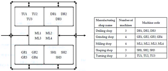
Figure 1.
Existing manufacturing configuration.
Consequently, with the aid of technology and operations experts, four cell-based configurations (obtained by different combinations of the existing machines) were identified. The EMS consisted of a process type layout, involving a total of 17 conventional machines arranged as per the process type. The alternative configurations, that is, cellular manufacturing configurations, CMS1, CMS2, CMS3, and CMS 4, were established as shown in Figure 2. The CMS1 and CMS2 were composed of 17 traditional machines grouped in 8 and 3 cells, respectively formed using a genetic algorithm [61]. Likewise, the CMS3 consisted of 17 traditional machines arrayed in 5 cells utilizing the rank order clustering algorithm [62] while the CMS4 was made up of 17 conventional machines clustered in 4 cells by employing a bond energy algorithm [63,64].
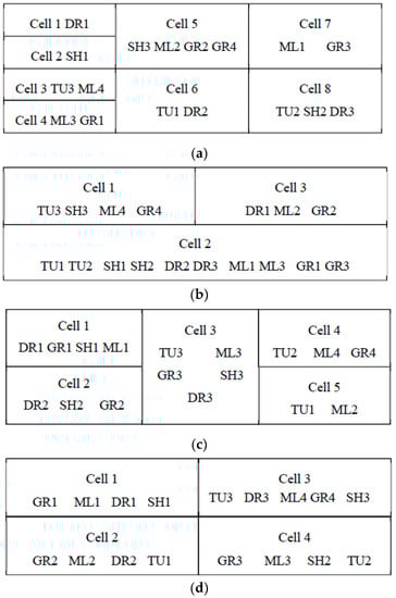
Figure 2.
Alternative manufacturing configurations: (a) CMS1, (b) CMS2, (c) CMS3, (d) CMS4.
Subsequently, five different alternatives needed to be evaluated to obtain the best configuration based on the given requirements. To assess different configurations, the production experts had to consider multiple performance measures and identify the best. Therefore, a systematic approach, which could establish the competitiveness of each alternative configuration, was mandatory. In a nutshell, the problem at hand could be described as the evaluation and ranking of alternative manufacturing configurations, depending on different performance measures.
4. Adopted MCDM Approach
In this section, three methodologies utilized in this work (FAHP, PROMETHEE, and VIKOR) are presented. At the outset, the simulation models of five configurations were developed. The performance of these configurations was computed through simulation experiments by establishing different scenarios. Accordingly, the MCDMs based on PROMTHEE [19,65,66] and VIKOR [67] were adopted to rank the alternative manufacturing configurations.
4.1. Fuzzy Analytic Hierarchy Process
The FAHP, which was originally suggested by Chang [68], was employed to compute the weights. The primary objective behind the application of the fuzzy set concept was dealing with uncertainty owing to imprecision or vagueness in decision making. The various steps of FAHP can be described as follows [69,70].
Step 1. Pairwise Comparison Matrix
A pairwise comparison matrix (employing AHP) was constructed using the Saaty 1–9 scale [71] as shown in Table 2.
Table 2.
Saaty 1–9 scale [66].
Step 2. Fuzzification
In this step, the fuzzified pairwise comparison matrix was generated using triangular fuzzy numbers (TFNs) as depicted in Figure 3. It meant the crisp numeric values obtained using AHP were transformed into fuzzy numbers. The TFNs can be described using Equation (1):
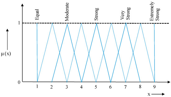
Figure 3.
Conversion of numerical values into fuzzy numbers.
The parameters l, m, and u represent the smallest, the most promising, and the largest values, respectively.
Step 3. Computation of fuzzy weights
The geometric mean was exploited to estimate the fuzzy weights using Equations (2) and (3):
Fuzzy geometric value, ri = [(l1 ⊗ l2 ⊗ …, ⊗li)1/i, (m1 ⊗ m2 ⊗ …, ⊗ mi)1/i, (u1 ⊗ u2 ⊗ …, ⊗ ui)1/i],
Fuzzy weights, wi = ri ⊗ (r1 ⨁ r2 ⨁ … ⨁ ri)−1.
Step 4. Defuzzification
This procedure transformed the fuzzy set or fuzzy number into crisp values or numbers utilizing Equation (4). The center-of-area method was utilized in this paper [72,73]:
Step 5. Normalization
The weights were normalized using Equation (5) to get the weighted total as 1:
4.2. Vikor Method
The different steps required to perform VIKOR-based MCDM methods are explained in this section [21]. Assume that there are m alternatives Si (i = 1, 2, …, m) and n attributes Aj (j = 1, 2, …, n). The primary idea of the VIKOR technique is to identify the positive and negative ideal points in the solution space.
- Step 1. Identify the decision matrix X = (xij)m×n, where xij represents real numbers defining the values of the jth attribute for the choice i.
- Step 2. Obtain the normalized decision matrix, (rij)m×n, using Equation (6):
- Step 3. Estimate the maximum and minimum values in the normalized decision matrix by employing Equations (7) and (8):
- Step 4. Determine the distance of alternatives to the optimal solution, that is, the utility measure (Si) and regret measure (Ri), using Equations (9) and (10), respectively:
- Step 5. Calculate the Qi (rank indexes) values utilizing Equation (11):where S+ = ; S− = ; R+ = ; and R− = , ∈ [0, 1] represents the weight for the policy of “the majority criteria” (or “the maximum group utility”).The excellence ranking will depend on the Si values and the worst rankings will follow the Ri values.
- Step 6. Prioritize the alternatives depending on the Qi values (arranged in increasing order).
In the VIKOR approach, a compromise solution is proposed for the alternative, which is the best ranked through Q (minimum) in case the succeeding two assumptions are fulfilled [21,74]:
C1. Agreeable advantage
Q1 − Q2 ⩾ DQ, where i = 2 is the second-best ranked choice in the order using Q and DQ = 1/(m − 1).
C2. Agreeable stability in decision making
The preference i = 1 must also be the best ranked by R and/or S. If either of the assumptions is not achieved, then a group of compromise solutions is suggested.
- Alternatives i = 1 and i = 2 if only hypothesis C2 is not fulfilled; or
- Alternatives i = 1, 2, …, m, if the hypothesis C1 is not fulfilled, where m is obtained through the correlation QM − Q1 < DQ, for maximum i.
4.3. PROMETHEE
The information for the PROMETHEE approach is a decision matrix comprising an array of possible choices [75]. The PROMETHEE ranks various alternatives depending on the partial ranking, with the following dominance flows, for the positive outranking flow [2]. Suppose that there are m alternatives Si (i = 1, 2, …, m) and n attributes Aj (j = 1, 2, …, n).
- Step 1. Determine the decision matrix X = (xij)m×n, where xij symbolizes the performance score characterizing the values of the jth attribute for the alternative i.
- Step 2. Identify beneficial (needs to be maximized) and non-beneficial (needs minimization) attributes.
- Step 3. In this step, two alternatives at a time are compared for a particular performance measure. The objective is to find out which alternative is better compared to the other alternatives and what the preference value is. The preference value is obtained based on the preference function opted for that performance measure. The different shapes of preference functions, such as usual, U-shape, V-shape, level, linear, Gaussian, etc., are available in Visual PROMETHEE to accommodate most practical situations.
- Step 4. The preference value for each pair of a particular performance measure is estimated as mentioned in Step 3. Since there are generally multiple performance criteria, a global degree of preference, irrespective of performance measures, is estimated. For example, for a pair of S1 and S2, the global degree of preference value is estimated using the following Equation (12):
In the equation, w1, w2, w3,..., wn are the normalized weights allocated to performance measure criteria A1, A2, A3,…., An, respectively. Aj (S1, S2) is the preference value for the pair (S1, S2) for the performance measure ‘j’.
It can be concluded here that the preference between two alternatives should depend on the global degree of the preference value. If the global degree of the preference value (∏(S1, S2)) is equal to zero, then S1 can never even be slightly preferred over S2. Secondly, if (∏(S1, S2)) is equal to one, then S1 should always strongly preferred to S2. Thirdly, if (∏(S1, S2)) is very close to zero but not exactly zero, then S1 has a weak preference over S2. Lastly, if (∏(S1, S2)) is approximately equal to one but not exactly one, then it means S1 has a strong preference over S2.
- Step 5. As stated in the above step, the obtained global degree of preference values for every pair of alternatives is used to get the positive, negative, and net flow for an alternative. For an alternative S1 positive flow, the negative flow and the net flow can be computed as in Equations (13)–(15), respectively:Phi+(S1) = ∏(S1,S2) + ∏(S1,S3) … + ∏(S1,Sm),Phi−(S1) = ∏(S2,S1) + ∏(S3,S1) … + ∏(Sm,S1),Phi(S1) = Phi+(S1) − Phi−(S1).
- Step 6. After computing the net flow values for each alternative, the alternatives are arranged in descending order. The alternative with the higher net flow is preferred over the other alternatives.
5. Implementation
The different MCDM methods that were practiced to obtain the solution for the discussed problem are explained in this section.
5.1. Simulation Model
The different manufacturing configurations (simulation model) were virtually developed before implementing the MCDM approaches. The alternative manufacturing configurations were simulated in ProModel 6.2 (ProModel Corporation, Ann Arbor, USA). In total, 24 scenarios were established as shown in Table 3 for the simulation of the current and newly remodeled alternative manufacturing configurations. The developed simulation model had the following characteristics:
Table 3.
Scenarios generated for the modeling of manufacturing configurations.
- The arrival of clients with mean inter-arrival times was considered at a random interval of times.
- Any number of orders could be placed by the arriving client.
- Any combination of products in the required quantities could be specified.
- Due dates were also assigned to the arriving order.
- The products in each order were machined using different machines depending on the routing strategy and the process plan.
- Different rules were employed to set up the product sequence on the machine.
The performance attributes that focused on customers as well as the system were considered in this study. Therefore, performance measures concerning machine utilization (MU), throughput time (TT), product blocking time (BT) (system-centric), and the earliness (ET) and lateness of products (LT) (customer-centric) were estimated in the simulation model. The evaluating attributes were identified to accomplish the objective of sustainable manufacturing regarding effective machine utilization, optimal space requirements, proper inventory management, higher customer satisfaction, reduced idle time, etc. In this investigation, the affinity between configurability and sustainability was explored in terms of system flexibility and utilization. Certainly, modularization and reconfiguration are crucial to attaining sustainable manufacturing, as emphasized in [76]. Finally, the simulation outcomes were utilized to evaluate the competitiveness of the various manufacturing configurations. The alternative schemes and scenarios were created depending on the following assumptions. For example, M3F1O1B1 represented a scheme in which the mean arrival time between clients was 3 days, an average of 1 order was placed by the client, the lot size for processing was 25, and the first-come-first-serve rule was followed.
- M3: Mean arrival time between clients—3 days.
- M4: Mean arrival time between clients—4 days.
- O1: Average orders per client—1.
- O2: Average orders per client—2.
- O3: Average orders per client—3.
- F1: First to arrive is dealt with first.
- F2: Processing time is shortest.
- B1: Lot of 25 parts.
- B2: Lot of 50 parts.
Five virtual (simulation) models, each representing five different manufacturing configurations, were established. The simulation models were exercised for various operating scenarios. The simulation results related to the scheme M3F1O1B1, for five alternative configurations, can be seen in Table 4. Certainly, there were inconsistencies in the performances of the various configurations depending on the five criteria. It can be observed that a particular configuration could not be selected based on this information because each configuration was good either in one or the other performance aspect. It can be inferred here that no one configuration was best on all five criteria. Hence, it was reasonable to employ a suitable outranking MCDM technique.
Table 4.
Simulation outcomes of five setups for scheme M3F1O1B1.
Since the objective was to evaluate five alternative configurations, the problem was therefore formalized as:
A = {existing manufacturing configuration (EMS), cellular manufacturing configuration 1 (CMS1), cellular manufacturing configuration 2 (CMS2), cellular manufacturing configuration 3 (CMS3), cellular manufacturing configuration 4 (CMS4)}
Five performance measuring criteria were utilized to evaluate these alternatives. The set of performance measuring criteria with their objective stated in the respective bracket is as follows:
P = {MU(maximization), ET(maximization), TT (minimization), LT (minimization), BT (minimization)}
The objective was to evaluate five alternative configurations for 24 different scenarios. Therefore, the overall performance score was computed by averaging the values in all 24 scenarios for the respective performance and the manufacturing configuration (see Table 5).
Table 5.
Overall performance score for different manufacturing configurations (decision matrix).
5.2. Weight Computation
The weights were computed using FAHP in this step. The AHP was utilized to obtain each attribute’s importance by generating a pairwise comparison matrix, as depicted in Table 6. In all, three pairwise comparison matrices for three decision-makers (D1, D2, D3) were obtained. The reason for taking suggestions from more than one expert was to combine their judgments to eliminate any bias.
Table 6.
Pairwise comparison matrices from various decision-makers.
Saaty [71] also defined consistency ratio, CR, to determine the amount of allowed discrepancy in a judgment. Therefore, the CR was also estimated for each specialist to confirm if the decision made by them was acceptable or not. It was confirmed that the CR value for three decision-makers, D1 (7.85%), D2 (8.10%), and D3 (9.82%), was less than 10%; therefore, the judgment made by them was consistent and acceptable.
Subsequently, the fuzzified pairwise comparison matrix was generated using TFNs as depicted in Table 7.
Table 7.
Fuzzified pairwise comparison matrices.
The fuzzy weights computed using the Equations (2) and (3) in Section 4.1 and are depicted in Table 8.
Table 8.
Computation of fuzzy weights.
Consequently, the fuzzy weights were defuzzified using Equation (4). The attributed weights estimated for each decision-maker were combined using the geometric mean [77] procedure as shown in Table 9.
Table 9.
Attribute weights obtained using FAHP.
5.3. VIKOR Application
In this step, the VIKOR-based MCDM technique utilizing the FAHP weight was implemented. It commenced with the definition of a normalized decision matrix (using Equation (6)) as evident in Table 10.
Table 10.
Decision matrix upon normalization.
Subsequently, the best values (vj+) in the normalized decision matrix were determined by employing Equations (7) and (8). The result for each criterion is shown in Table 11. The Si, Ri, and Qi values computed using Equations (9)–(11) for various alternatives can be seen in Table 12.
Table 11.
Best and worst values for the respective attributes.
Table 12.
Si, Ri, and Qi values for different alternatives.
5.4. PROMETHEE Employment
The PROMETHEE-based MCDM technique employing the FAHP weight was applied in this step. It commenced with the pairwise comparison as shown in Figure 4.
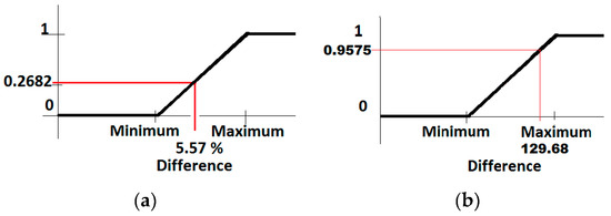
Figure 4.
Pairwise comparison of performance measure related to: (a) Machine utilization; (b) product lateness.
Since maximization was the objective for performance measure MU, CMS1 should be preferred over (better than) CMS4, whereas minimization was the objective for performance measure LT, therefore CMS4 was preferred over (better than) CMS1. Thus, in the pairwise comparison of CMS1 and CMS4 (refer to Table 7), the preference value was equal to (68.48147 − 62.97158)/(83.5133 − 62.97158) = 0.2682 (scheme M3F1O1B1). This meant CMS1 was 26.82% preferred over CMS4 for MU (refer to Figure 4). Whereas, for performance measure LT, the preference value was equal to (574.4222 − 444.7449)/(580.18 − 444.7449) = 0.9575. This meant CMS4 was 95.75% preferred over CMS1 for LT. Here, in the given problem, there were 24 scenarios, 5 performance measures, and 5 configurations, providing a total of 600 pairs of evaluation. Since a larger mathematical computation was needed for many pairwise comparisons, visual promethee software was preferred to do the pairwise comparisons.
In pairwise comparison of CMS1 and CMS4, the preference values with respect to each performance measure were estimated as PMU(CMS1, CMS4) = 0.2682; PET(CMS4, CMS1) = 0.5999; PTT(CMS4, CMS1) = 0.9575; PLT(CMS4, CMS1) = 0.0.6646; and PBT(CMS4, CMS1) = 0.4725. Normalized weights were set for each performance measure (as WMU = 0.163; WET = 0.210; WTT = 0.354; WLT = 0.123; WBT = 0.150).
The global preference value for pair ∏(CMS1, CMS4) was computed as 0.0437 and ∏(CMS4, CMS1) was equal to 0.6175.
The estimated positive, negative, and net flow score for configuration CMS1 are presented in Figure 5.
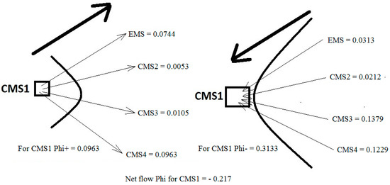
Figure 5.
Positive, negative, and net flow score for the configuration CMS1.
Table 13 depicts the positive, negative, and net flow score computed for different configurations, considering the average performance scores.
Table 13.
Positive and negative preference flows and ranking.
5.5. Sensitivity Analysis
The sensitivity analysis was executed to analyze changes in the output of the system model because of modifications in input parameter values [78,79]. It can be defined as a technique to understand the variation of input values on the final model results [80,81]. The most commonly used sensitive analysis is accomplished by varying the weights of the performance criteria or measures and analyzing the change in results [82]. It suggests that the model is stable and dependable if the solution is not very responsive to variations in the input. Therefore, in the suggested approach, the mutation in the weights of five performance measures was utilized to approve the model. Two designs of criteria weights, as demonstrated in Table 14, were employed for the sensitivity analysis. In design 1, machine utilization was assigned the highest importance, succeeded by earliness and the remaining performance measures. However, in design 2, the weights were computed by employing the entropy weight method [83,84].
Table 14.
Set of weights for sensitivity analysis.
6. Results
According to the VIKOR ranking method, the cellular manufacturing configuration “CMS3” was ranked the best, followed by CMS4, CMS2, CMS1, and EMS (see Table 12). In VIKOR, a compromised solution has to be proposed; therefore, two conditions must be checked, as discussed in Section 4.2. Since Q (CMS4) − Q (CMS3) = 0.0828 and DQ = 0.25, condition 1 (acceptable advantage) was not satisfied. It was not possible to distinguish the best one between CMS3 and CMS4. However, the alternative best ranked one depending on Q values was also best ranked by R and S. It suggests that condition 2 was satisfied. Henceforth, CMS3 and CMS4 were members of the compromise group (because Q (CMS4) − Q (CMS3) < DQ), but the alternative CMS2 could be considered in the compromise group because of Q (CMS2) − Q (CMS3) > DQ. Finally, depending on the VIKOR method, CMS3 could be suggested as the best configuration. The VIKOR method was again employed after removing the CMS4 configuration, leading to the following ranking of CMS3 > CMS2 > CMS1 > EMS. It also satisfied both acceptability criterion.
Similarly, using the PROMETHEE ranking method, the cellular manufacturing configuration “CMS3” was also ranked the best, followed by CMS4, CMS2, CMS1, and EMS, (see Table 13), which is in agreement with the VIKOR method.
Moreover, the results computed in the sensitivity analysis identified that the model was not very sensitive to variations in weights. The outcomes of the sensitivity analysis are reported in Table 15. Thus, it can be deduced that the model was robust and reliable as it exhibited inappreciable variations in output with modifications in the input weights.
Table 15.
Results of the sensitivity analysis.
7. Conclusions
An uncertain and competitive business environment makes industrial practitioners seek flexible approaches in manufacturing strategies. The competitive industrial practitioners adopt several strategies for invariable market situations, where persistent changes in design, as well as demand, seldom occur. The application of MCDM in RCMS was presented in this work. Indeed, the study in this paper was concerned with the manufacturing setup that requires reconfiguration for sustainable operations. The primary challenge in the integration of RCMS and sustainability is the evaluation of all possible alternatives and thereby selecting the best in terms of optimum requirements for specific internal and external market demands.
In this paper, the effect of demand patterns, scheduling rules, and lot sizes were employed to achieve sustainability and enhance effectiveness in terms of system utilization, throughput time, earliness of customer demand satisfaction and lateness of customer demand delivery, and time for which the customer demands are blocked in the system. This work aimed to alleviate irrelevant actions using productive RCMS configuration by achieving enhanced machine utilization, as well as by minimizing tardiness and product blocking times. In previous studies, the majority of techniques have relied on conventional approaches, but this work focused on uncertainty concepts, such as fuzzy AHP. It was also noticed that the utilization of PROMETHEE and VIKOR combined with FAHP in RCMS is still insufficient. Therefore, the prominence of PROMETHEE [58] and VIKOR [59,60] have increased in many fields and this paper introduced decision-making models that can determine rational RCMS policies for the sustainable development of an existing manufacturing system. A total of 24 possible alternative demand scenarios were analyzed based on external demands (that included the arrival pattern of clients and number of orders per client) and internal demands (such as the scheduling rule and lot size). The performance criteria were averaged for various configurations and the resultant outcomes were utilized to assist in the decision-making (MCDM) procedure.
In this work, the MCDM approaches based on PROMETHEE and VIKOR were implemented to rank different configurations. The FAHP was employed to estimate the weights of different performance measures. The simulation outcomes for various configurations were examined by utilizing FAHP-PROMETHEE and FAHP-VIKOR. A cellular manufacturing system with 17 conventional machines arranged in 5 cells (CMS3) (Figure 2) was found to be the best alternative for sustainable operations using both the techniques. It suggests that CMS3 configuration can efficiently and effectively satisfy the requirements of all considered decision-makers. The configuration CMS3 attained a well-balanced performance in terms of all aspects, namely machine utilization (optimal resource consumption), throughput time (higher customer satisfaction), earliness, lateness and blocking time (minimal non-value-added activities), space and inventory management, etc. The CMS3 layout could achieve 66.53% machine utilization, and 156.33 h of earliness, including minimal lateness hours (513.31 h), blocking time (844.53 h), and throughput time (898.94 h). The other configurations (CMS1, CMS2, and CMS 4) were also good, but they performed exceptionally in one or two aspects, but in the rest, they had inadequate performance. For instance, the configuration CMS2 performed supremely in machine utilization but was unable to achieve satisfactory blocking time, throughput time, lateness hours, etc. Henceforth, multiple criteria, as specified by different stakeholders, can be fulfilled using CMS3. It means a single configuration is sufficient for multiple customers and further reconfiguration for a given customer can be avoided, thus saving adequate cost and additional resource wastage. Moreover, similar outcomes from the two techniques also established their reliability and robustness to overcome any uncertainty in the system. Based on the sensitivity analysis, it was validated and confirmed that the presented model was robust and steady.
It is believed that this study would provide an alternative viewpoint to those who want to explore different production configurations for achieving lean, sustainable, and agile manufacturing. Cellular manufacturing and the philosophy of work cells are at the core of lean and agile manufacturing. Their gains are numerous and diverse. Cellular manufacturing simplifies material flow and resource management as well as aiding in achieving sustainability. However, it is mandatory to examine various reasonable cell-based alternatives while inducing any amendment. There is a notable threat to change to any other production setup before evaluating various alternatives. The adopted simulation technique is valuable for generating distinctive scenarios and analyzing the feasible consequences beforehand. The outcomes acquired using simulation need to be reviewed properly, particularly if the choices involve multiple performance measures. Thus, for organizations that aim for lean production and sustainable manufacturing, the approach presented in the paper is helpful in identifying and ranking desirable configurations as a substitute to the existing manufacturing system. The development of a procedure that can assess the distinct alternative configurations in light of the cost and risk associated with cell-based reconfiguration is a topic of future research.
Author Contributions
Conceptualization, A.U.R. and S.H.M.; methodology, A.U.R. and S.H.M.; software, A.U.R. and Y.S.U.; validation, A.U.R., S.H.M. and U.U.; formal analysis, S.H.M.; investigation, S.H.M. and U.U.; resources, U.U. and Y.S.U.; data curation, A.U.R., Y.S.U. and U.U.; writing—original draft preparation, A.U.R. and S.H.M.; writing—review and editing, S.H.M. and U.U.; supervision, A.U.R.; funding acquisition, A.U.R. and U.U.
Funding
This research was funded by Deanship of Scientific Research at King Saud University grant number [RG-1439-005].
Acknowledgments
The authors extend their appreciation to the Deanship of Scientific Research at King Saud University for funding this work through research group number RG-1439-005.
Conflicts of Interest
The authors declare no conflict of interest.
References
- Koren, Y. Reconfigurable manufacturing system: Key to future manufacturing. In Proceedings of the 1998 Japan-USA Symposium on Flexible Automation, Otsu, Japan, 1998; pp. 677–682. [Google Scholar]
- Mehrabi, M.G.; Ulsoy, A.G.; Koren, Y. Reconfigurable manufacturing systems: Key to future manufacturing. J. Intell. Manuf. 2000, 11, 403–419. [Google Scholar] [CrossRef]
- Dashchenko, A.I. Reconfigurable Manufacturing Systems and Transformable Factories; Springer Science & Business Media: Berlin, Germany, 2007; p. 731. [Google Scholar]
- Youssef, A.M.A.; El Maraghy, H.A. Assessment of manufacturing systems reconfiguration smoothness. Int. J. Adv. Manuf. Technol. 2006, 30, 174–193. [Google Scholar] [CrossRef]
- Bi, Z.M.; Lang, S.Y.T.; Verner, M.; Orban, P. Development of reconfigurable machines. Int. J. Adv. Manuf. Technol. 2008, 39, 1227–1251. [Google Scholar] [CrossRef]
- Vakharia, A.J.; Wemmerlov, U. Designing a Cellular Manufacturing System: A Materials Flow Approach Based on Operation Sequences. IIE Trans. 1990, 22, 84–97. [Google Scholar] [CrossRef]
- Arunagiri, A.; Marimuthu, U.; Gopalakrishnan, P.; Slota, A.; Zajac, J.; Paulraj, M.P. Sustainability Formation of Machine Cells in Group Technology Systems Using Modified Artificial Bee Colony Algorithm. Sustainability 2018, 10, 42. [Google Scholar] [CrossRef]
- Unglert, J.; Jauregui-Becker, J.; Hoekstra, S. Computational Design Synthesis of reconfigurable cellular manufacturing systems: A design-engineering model. Procedia CIRP 2016, 57, 374–379. [Google Scholar] [CrossRef]
- Shankar, K.M.; Kumar, P.U.; Kannan, D. Analyzing the Drivers of Advanced Sustainable Manufacturing System Using AHP Approach. Sustainability 2016, 8, 824. [Google Scholar] [CrossRef]
- Cheikh, S.B.; Hajri-Gabouj, S.; Darmoul, S. Manufacturing configuration selection under arduous working conditions: A multi-criteria decision approach. In Proceedings of the 2016 International Conference on Industrial Engineering and Operations Management, Kuala Lumpur, Malaysia, 8–10 March 2016; pp. 1280–1291. [Google Scholar]
- Ateekh-Ur-Rehman, A.U.R. Manufacturing Configuration Selection using Multi-Criteria Decision Tool. Int. J. Adv. Manuf. Technol. 2013, 65, 625–639. [Google Scholar] [CrossRef]
- Hasan, F.; Jain, P.K.; Kumar, D. Optimum configuration selection in Reconfigurable Manufacturing System involving multiple part families. OPSEARCH 2013, 51, 297–311. [Google Scholar] [CrossRef]
- Dou, X.J.; Dai, X.; Meng, Z. Graph theory-based approach to optimize single-product flow-line configurations of RMS. Int. J. Adv. Manuf. Technol. 2009, 41, 916–931. [Google Scholar] [CrossRef]
- Baker, D.; Bridges, D.; Hunter, R.; Johnson, G.; Krupa, J.; Murphy, J.; Sorenson, K. Guidebook to Decision-Making Methods; McGraw Hill Inc.: New York, NY, USA, 2001. [Google Scholar]
- Tabucanon, M.T. Multiple Criteria Decision Making in Industry; Elsevier: Amsterdam, The Netherlands, 1988; p. 339. [Google Scholar]
- Aruldoss, M.; Lakshmi, T.M.; Venkatesan, V.P. A survey on multi criteria decision making methods and its applications. Am. J. Inf. Syst. 2013, 1, 31–43. [Google Scholar]
- Behzadian, M.; Kazemzadeh, R.B.; Albadvi, A.; Aghdasi, M. PROMETHEE: A comprehensive literature review on methodologies and applications. Eur. J. Oper. Res. 2010, 200, 198–215. [Google Scholar] [CrossRef]
- Brans, J.P. L’ingéniérie de la décision. Elaboration d’instruments d’aide à la décision. Méthode PROMETHEE. In Nadeau, L’aide À La Décision: Nature, Instruments Et Perspectives D’avenir; Landry, R.M., Ed.; Presses de l’Université Laval: Québec, QC, Canada, 1982; pp. 183–214. [Google Scholar]
- Brans, J.P.; Vincke, P. A preference ranking organization method: The PROMETHEE method. Manag. Sci. 1985, 31, 647–656. [Google Scholar] [CrossRef]
- Brans, J.P.; Mareschal, B. The PROMCALC and GAIA decision support system for for multicriteria decision aid. Decis. Support Syst. 1994, 12, 297–310. [Google Scholar] [CrossRef]
- Opricovica, S.; Tzeng, G.-H. Compromise solution by MCDM methods: A comparative analysis of VIKOR and TOPSIS. Eur. J. Oper. Res. 2004, 156, 445–455. [Google Scholar] [CrossRef]
- Opricovica, S.; Tzeng, G.-H. Extended VIKOR method in comparison with outranking methods. Eur. J. Oper. Res. 2007, 178, 514–529. [Google Scholar] [CrossRef]
- Sakhuja, S.; Jain, V.; Dweiri, F. Application of an integrated MCDM approach in selecting outsourcing strategies in hotel industry. Int. J. Logist. Syst. Manag. 2015, 20, 304–324. [Google Scholar] [CrossRef]
- Jain, V.; Sangaiah, A.K.; Sakhuja, S.; Thoduka, N.; Aggarwal, R. Supplier selection using fuzzy AHP and TOPSIS: a case study in the Indian automotive industry. Neural Comput. Appl. 2018, 29, 555–564. [Google Scholar] [CrossRef]
- Noor, Z.M.; Md Fauadi, M.H.F.; Jafar, F.A.; Nordin, M.H.; Yahaya, S.H.; Ramlan, S.; Shri Abdul Aziz, M.A. Fuzzy Analytic Hierarchy Process (FAHP) Integrations for Decision Making Purposes: A Review. J. Adv. Manuf. Technol. 2017, 11, 139–154. [Google Scholar]
- Dani, A.R.; De, S.K. Fuzzy Analytical Hierarchical Process for Selecting a Bank. OPSEARCH 2003, 40, 241–251. [Google Scholar] [CrossRef]
- Samanlioglu, F.; Ayag, Z. A fuzzy AHP-PROMETHEE II-approach for evaluation of solar power plant location alternatives in Turkey. J. Intell. Fuzzy Syst. 2017, 33, 859–871. [Google Scholar] [CrossRef]
- Eguia, I.; Lozano, S.; Racero, J.; Guerrero, F. Cell design and loading with alternative routing in cellular reconfigurable manufacturing systems. In Proceedings of the 7th IFAC Conference on Manufacturing Modelling, Management, and Control International Federation of Automatic Control, Saint Petersburg, Russia, 19–21 June 2013; pp. 1744–1749. [Google Scholar]
- Padayachee, J.; Bright, G. A multi-period group technology method for dynamic cellular manufacturing systems. S. Afr. J. Ind. Eng. 2016, 27, 90–100. [Google Scholar] [CrossRef]
- ElMaraghy, H.A. Flexible and reconfigurable manufacturing systems paradigms. Int. J. Flex. Manuf. Syst. 2006, 17, 261–276. [Google Scholar] [CrossRef]
- Koren, Y.; Heisel, U.; Jovane, F.; Moriwaki, T.; Pritschow, G.; Ulsoy, G.; Van Brussel, H. Reconfigurable manufacturing systems. CIRP Ann. 1999, 48, 527–540. [Google Scholar] [CrossRef]
- Xing, B.; Nelwamondo, F.V.; Battle, K.; Gao, W.; Marwala, T. Application of Artificial Intelligence (AI) Methods for Designing and Analysis of Reconfigurable Cellular Manufacturing System (RCMS). In Proceedings of the 2nd International Conference on Adaptive Science & Technology, ICAST 2009, Accra, Ghana, 14–16 December 2009; pp. 402–409. [Google Scholar]
- Koren, Y.; Ulsoy, A.G. Vision, principles and impact of reconfigurable manufacturing systems. Powertrain Int. 2002, 3, 14–21. [Google Scholar]
- Mittal, K.K.; Jain, P.K. An Overview of Performance Measures in Reconfigurable Manufacturing System. Procedia Eng. 2014, 69, 1125–1129. [Google Scholar] [CrossRef]
- Azab, A.; Naderi, B. Modelling the problem of production scheduling for reconfigurable manufacturing systems. Procedia CIRP 2015, 33, 76–80. [Google Scholar] [CrossRef]
- Abbasi, M.; Houshmand, M. Production planning and performance optimization of reconfigurable manufacturing systems using genetic algorithm. Int. J. Adv. Manuf. Technol. 2011, 54, 373–392. [Google Scholar] [CrossRef]
- Bensmaine, A.; Dahane, M.; Benyoucef, L. A non-dominated sorting genetic algorithm based approach for optimal machines selection in reconfigurable manufacturing environment. Comput. Ind. Eng. 2013, 66, 519–524. [Google Scholar] [CrossRef]
- Yamada, Y.; Ookoudo, K.; Komura, Y. Layout Optimization of Manufacturing Cells and Allocation Optimization of Transport Robots in Reconfigurable Manufacturing Systems Using Particle Swarm Optimization. In Proceedings of the 2003 IEEE/RSJ International Conference on Intelligent Robots and Systems (IROS 2003), Las Vegas, NV, USA, 27–31 October 2003; pp. 2049–2054. [Google Scholar]
- Padayachee, J.; Bright, G. Synthesis of Evolving Cells for Reconfigurable Manufacturing Systems. Mater. Sci. Eng. 2014, 65, 012009. [Google Scholar] [CrossRef]
- Bass, F. A New Product Growth for Model Consumer Durables. Manag. Sci. 1969, 15, 215–227. [Google Scholar] [CrossRef]
- Eguia, I.; Molina, J.C.; Lozano, S.; Jesus Racero, J. Cell design and multi-period machine loading in cellular reconfigurable manufacturing systems with alternative routing. Int. J. Prod. Res. 2017, 55, 2775–2790. [Google Scholar] [CrossRef]
- Eguia, I.; Racero, J.; Guerrero, F.; Lozano, S. Cell Formation and Scheduling of Part Families for Reconfigurable Cellular Manufacturing Systems Using Tabu Search. Simul. Trans. Soc. Model. Simul. Int. 2013, 89, 1056–1072. [Google Scholar] [CrossRef]
- Abdi, M.R.; Labib, A.W. Feasibility study of the tactical design justification for reconfigurable manufacturing systems using the fuzzy analytical hierarchical process. Int. J. Prod. Res. 2004, 42, 3055–3076. [Google Scholar] [CrossRef]
- Singh, R.; Khilwani, N.; Tiwari, M. Justification for the selection of a reconfigurable manufacturing system: a fuzzy analytical hierarchy based approach. Int. J. Prod. Res. 2007, 45, 3165–3190. [Google Scholar] [CrossRef]
- Puik, E.; Telgen, D.; Moergestel, L.; Ceglarek, D. Assessment of reconfiguration schemes for Reconfigurable Manufacturing Systems based on resources and lead time. Robot. Comput. Integr. Manuf. 2017, 43, 30–38. [Google Scholar] [CrossRef]
- Wang, J.-W.; Cheng, C.-H.; Kun-Cheng, H. Fuzzy hierarchical TOPSIS for supplier selection. Appl. Soft Comput. 2009, 9, 377–386. [Google Scholar] [CrossRef]
- Hwang, C.L.; Yoon, K. Multiple Attribute Decision Making: Methods and Applications; Springer: Berlin/Heidelberg, Germany, 1981. [Google Scholar]
- Satty, T.L. Multi Criteria Decision Making: The Analytic Hierarchy Process; McGraw-Hill Inc.: New York, NY, USA, 1988. [Google Scholar]
- Torabi, S.A.; Shokr, I. A Common Weight Data Envelopment Analysis Approach for Material Selection. Int. J. Eng. Trans. C Asp. 2015, 28, 913–921. [Google Scholar]
- Govindan, K.; Jepsen, M.B. ELECTRE: A comprehensive literature review on methodologies and applications. Eur. J. Oper. Res. 2016, 250, 1–29. [Google Scholar] [CrossRef]
- Brans, J.P.; De Smet, Y. PROMETHEE Methods. In Multiple Criteria Decision Analysis; Greco, S., Ehrgott, M., Figueira, J., Eds.; International Series in Operations Research & Management Science; Springer: New York, NY, USA, 2016; Volume 233. [Google Scholar]
- Król, A.; Księżak, J.; Kubińska, E.; Rozakis, S. Evaluation of Sustainability of Maize Cultivation in Poland. A Prospect Theory—PROMETHEE Approach. Sustainability 2018, 10, 4263. [Google Scholar] [CrossRef]
- Hashemi, H.; Mousavi, S.M.; Zavadskas, E.K.; Chalekaee, A.; Turskis, Z. A New Group Decision Model Based on Grey-Intuitionistic Fuzzy-ELECTRE and VIKOR for Contractor Assessment Problem. Sustainability 2018, 10, 1635. [Google Scholar] [CrossRef]
- Abdi, M.R. Selection of a Layout Configuration for Reconfigurable Manufacturing Systems using the AHP. In Proceedings of the 8th International Symposium on the Analytic Hierarchy Process Multi-criteria Decision Making, Honolulu, HI, USA, 15–17 February 2005. [Google Scholar]
- Abdi, M.R. Fuzzy multi-criteria decision model for evaluating reconfigurable machines. Int. J. Prod. Econ. 2009, 117, 1–15. [Google Scholar] [CrossRef]
- Bensmaine, A.; Dahane, M.; Benyoucef, L. Process Plan Generation in Reconfigurable Manufacturing Systems using AMOSA and TOPSIS. In Proceedings of the 14th IFAC Symposium on Information Control Problems in Manufacturing, Bucharest, Romania, 23–25 May 2012; pp. 560–565. [Google Scholar]
- Mpofu, K.; Tlale, N.S. Multi-level decision making in reconfigurable machining systems using fuzzy logic. J. Manuf. Syst. 2012, 31, 103–112. [Google Scholar] [CrossRef]
- Brans, J.P.; Mareschal, B.; Figueira, J.; Greco, S.; Ehrgott, M. (Eds.) Multiple Criteria Decision Analysis: State of the Art Surveys; Springer Science + Business Media, Inc.: Berlin, Germany, 2005; pp. 163–196. [Google Scholar]
- Singla, A.; Ahuja, I.S.; Sethi, A.S. Comparative analysis of technology push strategies influencing sustainable development in manufacturing industries using TOPSIS and VIKOR Technique. Int. J. Qual. Res. 2007, 12, 129–146. [Google Scholar]
- Xu, F.; Liu, J.; Lin, S.; Yuan, J. A VIKOR-based approach for assessing the service performance of electric vehicle sharing programs: a case study in Beijing. J. Clean. Prod. 2017, 148, 254–267. [Google Scholar] [CrossRef]
- Wu, X.; Chu, C.-H.; Wang, Y.; Yan, W. A genetic algorithm for cellular manufacturing design and layout. Eur. J. Oper. Res. 2007, 181, 156–157. [Google Scholar] [CrossRef]
- Moona, G.; Kumar, A.; Kumar, H. Restructuring of a plant production layout by using different array-based clustering techniques. Int. J. Adv. Oper. Manag. 2016, 8, 153–167. [Google Scholar] [CrossRef]
- Khanna, K.; Kumar, R. Part family and operations group formation for RMS using bond energy algorithm. Int. J. Eng. Technol. 2017, 9, 1365–1373. [Google Scholar] [CrossRef]
- Huang, S.; Yan, Y. Part family grouping method for reconfigurable manufacturing system considering process time and capacity demand. Flex. Serv. Manuf. J. 2019, 31, 424–445. [Google Scholar] [CrossRef]
- Brans, J.P.; Mareschal, B.; Vincke, P. How to select and how to rank projects: The PROMETHEE method for MCDM. Eur. J. Oper. Res. 1986, 24, 228–238. [Google Scholar] [CrossRef]
- Dulmin, R.; Mininno, V. Supplier selection using a multicriteria decision aid method. J. Purch. Supply Manag. 2003, 9, 177–187. [Google Scholar] [CrossRef]
- Kumar, M.; Samuel, C. Selection of Best Renewable Energy Source by Using VIKOR Method. Technol. Econ. Smart Grids Sustain. Energy 2017, 2, 8. [Google Scholar]
- Chang, D.Y. Applications of the extent analysis method on fuzzy AHP. Eur. J. Oper. Res. 1996, 95, 649–655. [Google Scholar] [CrossRef]
- Wang, C.-N.; Nguyen, V.T.; Thai, H.T.N.; Duong, D.H. Multi-Criteria Decision Making (MCDM) Approaches for Solar Power Plant Location Selection in Vietnam. Energies 2018, 11, 1504. [Google Scholar] [CrossRef]
- Naghadehi, M.Z.; Mikaeil, R.; Ataei, M. The application of fuzzy analytic hierarchy process (FAHP) approach to selection of optimum underground mining method for Jajarm Bauxite Mine, Iran. Expert Syst. Appl. 2009, 36, 8218–8226. [Google Scholar] [CrossRef]
- Saaty, T.L. The Analytic Hierarchy Process: Planning, Priority Setting, Resources Allocation; McGraw-Hill: New York, NY, USA, 1980. [Google Scholar]
- Ayhan, M.B. A fuzzy AHP approach for supplier selection problem: A case study in a gearmotor company. Int. J. Manag. Value Supply Chain. (IJMVSC) 2013, 4, 11–23. [Google Scholar] [CrossRef]
- Ishizaka, A. Comparison of Fuzzy logic, AHP, FAHP and Hybrid Fuzzy AHP for new supplier selection and its performance analysis. Int. J. Integr. Supply Manag. 2014, 9, 1–22. [Google Scholar] [CrossRef]
- Acuña-Soto, C.M.; Liern, V.; Pérez-Gladish, B. A VIKOR-based approach for the ranking of mathematical instructional videos. Manag. Decis. 2018, 57, 501–522. [Google Scholar] [CrossRef]
- Mladineo, M.; Jajac, N.; Rogulj, K. A simplified approach to the PROMETHEE method for priority setting in management of mine action projects. Croat. Oper. Res. Rev. 2016, 7, 249–268. [Google Scholar] [CrossRef]
- Bi, Z.; Liu, Y.; Baumgartner, B.; Culver, E.; Sorokin, J.; Peters, A.; Cox, B.; Hunnicutt, J.; Yurek, J.; O’Shaughnessey, S. Reusing industrial robots to achieve sustainability in small and medium-sized enterprises (SMEs). Ind. Robot 2015, 42, 264–273. [Google Scholar] [CrossRef]
- Forman, E.; Peniwati, K. Aggregating Individual Judgments and Priorities with the Analytic Hierarchy Process. Eur. J. Oper. Res. 1998, 108, 165–169. [Google Scholar] [CrossRef]
- Simanaviciene, R.; Ustinovichius, L. Sensitivity Analysis for Multiple Criteria Decision Making Methods: TOPSIS and SAW. Procedia Soc. Behav. Sci. 2010, 2, 7743–7744. [Google Scholar] [CrossRef]
- Triantaphyllou, E.; Sanchez, A. A Sensitivity Analysis Approach for Some Deterministic Multi-Criteria Decision-Making Methods. Decis. Sci. 1997, 28, 151–194. [Google Scholar] [CrossRef]
- Leonelli, R.B. Enhancing a Decision Support Tool with Sensitivity Analysis, Project Background Report. Master’ Thesis, University of Manchester, School of Computer Science, Manchester, UK, 2012; pp. 1–29. [Google Scholar]
- Syamsuddin, I. Multicriteria Evaluation and Sensitivity Analysis on Information Security. Int. J. Comput. Appl. 2013, 69, 22–25. [Google Scholar] [CrossRef]
- Chen, Y.; Yu, J.; Shahbaz, K.; Xevi, E. A GIS-Based Sensitivity Analysis of Multi-Criteria Weights. In Proceedings of the 18th World IMACS/MODSIM Congress, Cairns, Australia, 13–17 July 2009; pp. 3137–3143. [Google Scholar]
- Zhi-Hong, Z.; Yi, Y.; Jing-Nan, S. Entropy method for determination of weight of evaluating in fuzzy synthetic evaluation for water quality assessment indicators. J. Environ. Sci. 2006, 18, 1020–1023. [Google Scholar]
- Guo, S. Application of entropy weight method in the evaluation of the road capacity of open area. AIP Conf. Proc. 2017, 1839, 020120. [Google Scholar] [CrossRef]


© 2019 by the authors. Licensee MDPI, Basel, Switzerland. This article is an open access article distributed under the terms and conditions of the Creative Commons Attribution (CC BY) license (http://creativecommons.org/licenses/by/4.0/).