Abstract
China is the largest emitter of carbon dioxide (CO2) in the world, and the Chinese government has accordingly proposed a series of measures to achieve a low-carbon economy. Due to the low carbon emission performance (CEP) and the high industry portion of the northern provinces in China, evaluating the CEPs of industrial sectors in northern China is necessary. By considering the different CEP assessments in regional and industrial research, a dual-perspective assessment of CEP was presented to narrow the gap between the regional and industrial perspectives. The dual model of slack-based measure (SBM) and data envelopment analysis (DEA) was combined with the global Malmquist–Luenberger index (GMLI) proposed to measure the static CEP and the dynamic change of the CEP of six provinces in northern China from 2006–15 for the regional and industrial perspectives, respectively. A comparison of the results under the different perspectives proved the irrationality of our evaluation under the sole perspective. For example, for Jilin Province, the CEPs of Mining and Processing of Nonmetal and Other Ores (Sector 4) ranked in the top 30% in the regional perspective. However, in the industrial level, the CEPs of Mining and Processing of Nonmetal and Other Ores (Sector 4) ranked lower. The CEPs of the Production and Supply of Electric Power and Heat Power (Sector 20) of Heilongjiang Province ranked in the bottom 30% in a regional perspective but ranked first at the industrial level. We also found the advantage sectors in the CEP under the region–sector dual perspective. For example, for Jilin Province, the Processing of Petroleum, Coking, and Processing of Nuclear Fuel (Sector 10) and the manufacture of Transport Equipment (Sector 16) were the advantageous sectors. The dual-perspective assessment aimed to evaluate the CEP under diverse views. It also provided a more reliable path to reduce CO2 emissions for managers and regulators.
1. Introduction
Climate change caused by carbon emissions presents severe challenges to human welfare [1,2]. Since the UK proposed the initiative of developing a “low-carbon economy” in 2003, reducing carbon dioxide (CO2) emissions, improving carbon emission performance (CEP), and creating a low-carbon economy have gained consensus from all countries in the world [3]. Nowadays, China has become the largest emitter of CO2 in the world [4,5]. Inevitably, China’s CO2 emissions will constantly increase in the future. Therefore, China’s CO2 emission reduction research has great significance for climate change globally [6,7]. To achieve the goal of CO2 emission reduction, China first promised in 2009 to decrease its CO2 emissions per unit of GDP in 2020 by 40%–45% compared with the 2005 level [8]. Following that, China reiterated the control goal of CO2 emission in 2015 to lower CO2 emissions per unit of GDP in 2030 by 60%–65% compared with the 2005 level [9]. Given that northern China has the higher CO2 emissions and the industry is the primary support of national economic development, it is vital for the country to control CO2 emissions in the northern area [10]. Therefore, scientifically and reasonably measuring the CEP of industrial sectors in northern China is necessary for promoting the development of the green industry and a low-carbon economy.
Two methods are used to evaluate the CEP: the single-factor CEP and the total-factor CEP [11,12]. The first method is mainly based on carbon intensity (CO2 emissions per unit of gross domestic production) [13,14,15], carbon emission per capita [16,17,18], total CO2 emission (calculated by taking a country [a region] as a unit), and carbon productivity (reciprocal of carbon intensity) [19,20]. This method has the advantages of simple application and clear indication, but it overlooks the effects of input factors, such as labor, energy, and capital [21]. Thus, some researchers used the total-factor CEP method to consider relationships between carbon, energy, and economy in CEP evaluation. Therefore, total-factor CEP has been widely used for CEP assessment. The total-factor CEP includes two different techniques: stochastic frontier analysis (SFA) [22,23] and data envelopment analysis (DEA) [24]. SFA is a parameter method that often employs a specific function to identify the production frontier. For example, Herrala and Goel adopted SFA to examine the CEP in 170 countries during 1997–2007 and found vast differences in the efficiency levels and efficiency changes across countries [25]. Dong et al. employed the trans-log SFA to examine the regional CEP. The results showed that the CEP in China is rising and the CEP of eastern China was higher than that of central and western China [26]. Although SFA has been widely applied, the outcomes are often easily affected by the selected production function in the above research [27]. Consequently, building a suitable production function is a bottleneck in SFA research. On the contrary, no such problem exists with the DEA method. DEA is a non-parameter method that does not need to set up a production function or conduct dimensionless quantitative processing of data. When using DEA to measure carbon emission performance, we first utilize linear programming and convex analysis to construct a production frontier, after which we assess the relative efficiency of a decision-making unit (DMU) by comparing the distance deviating from the production frontier [28]. DEA is superior to SFA in terms of sensitivity and scope of application, and it can deal with unexpected output and dynamic changes more scientifically [29,30]. Thus, mainly by emphasizing the industrial and regional perspectives, DEA has gained considerable popularity for CEP evaluation.
From the industrial perspective, extensive research has been conducted on the overall CEPs of different countries. For instance, Zhou et al. used DEA to measure the CEPs of the 18 top emitter countries during 1997–2004 [24]. Wang et al. adopted the DEA method to measure CEPs in 123 countries during 1992–2009. The CEPs of developing countries are thus found to be lower than those of developed countries [31]. Similarly, Wang et al. [8,32] reached a consistent conclusion. To further explore the reasons of low CEP in China, some scholars attempted to measure the CEPs of China at the provincial level. Wang et al. [33] used the method of Zhou et al. [24] to measure the CEP of Chinese provinces. After this study, a numerous CEP studies of Chinese provinces were carried out using DEA models. Lin et al. applied a recently developed non-radial directional distance function to evaluate China’s regional CEP between 1997 and 2009. Their work established that the provinces in the east generally performed better than those in the central and western regions [34]. Zhong et al. [35] and Wang et al. [36] also obtained similar conclusions. To further examine the CEP of different cities, Zhou et al. [37] used the DEA method to measure the CEP of 71 Chinese cities during 2005–2012. Their results showed that the CEP in the east was higher than those in the central and western regions. Moreover, technological progress drove the change of the CEP. They further confirmed that the CEP of the eastern regions were higher than those of the central and western regions. The above results verified the overall CEP of each region, but did not investigate the CEPs of specific industries. Therefore, to fill this gap, researchers have studied the CEPs of different sectors, such as agriculture [38], construction [39], transportation industry [40,41], logistics industry [42], industry [43] and industrial sector [44,45,46,47,48]. Due to the large quantities of carbon emissions caused by the industrial sector, most investigations focused on the industry-level CEP analysis of China. For example, Wu et al. [49] adopted DEA to measure the industrial CEPs in different regions of China. CEPs in the east were higher than those in the central and western regions. Zhang et al. [1] adopted DEA and Moran’s Index to evaluate the industrial CEPs of 30 provinces in China during 2005–12. The outcomes revealed that the CEPs of all 30 regions were generally lower, especially in the northwest. The findings presented by Cheng et al. were similar [43,50]. Given the above research, we can only obtain the CEP rank and potential emission reduction from the perspective of a single industry. Providing a quantitative analysis for improving the CEP from the regional perspective has remained a challenging task. Meanwhile, examining the rank of CEPs in different regions without the consideration of the quantitative driver analysis proved to be insignificant for the reduction of carbon emissions.
From a regional perspective, some scholars analyzed the CEPs of the industrial sectors in a single region. For example, Xie et al. [51] applied a DEA model to measure the CEPs of 37 industrial sectors in China from 2005 to 2014. The result indicated that an obvious heterogeneity of industries in terms of CEPs. Zhang et al. [52] proposed the non-radial global Malmquist CEP index to measure the dynamic changes in the CEPs of 38 sectors in China from 1990 to 2012. They found that the catch-up effect and innovations drove the changes in the CEP. Yu et al. [53] used the DEA method to evaluate the CEPs of 24 industrial sectors in China from 1995 to 2015. Their findings indicated that the difference in the CEPs of 24 industrial sectors gradually decreased during the study period. The above studies examined the CEPs of different industrial sectors in a region and filled the gap in relation to the industrial perspective. However, we cannot compare the CEPs of different sectors due to the various technologies in industries.
Prior research have focused on either the industrial or the regional perspective, but do not consider a dual perspective. To fill the gap, Wang et al. [54] applied a DEA analysis method to estimate the CEPs of the primary, secondary, and tertiary industries of 30 provinces. The CEP of the eastern region was found to be higher than that of the central and western regions, and the CEP in tertiary industries is greater than that in the primary and secondary industries. In summary, from the regional perspective, the ranking of CEPs of different industrial sectors in a region is insignificant for improving the CEP without considering the industrial structure. From the industrial perspective, the ranking of the CEPs of the same industrial sector in different regions is unreasonable given the different techniques used and the variations in economic development levels. Current investigations on the regional and industrial perspectives only discussed the primary, secondary, and tertiary industries. Accordingly, the nonparametric method was adopted to evaluate the CEPs of northern provinces in China from the region–sector dual perspective. The CEPs of industrial sectors in the northern regions was measured accordingly. For the regional perspective, we measured the CEPs of different industrial sectors in a region. For the industrial perspective, we calculated the CEPs of the same industrial sectors from different provinces with consideration of the top and average development levels. By coupling the regional CEPs with those of the industrial sectors, we identified the industrial sectors with low CEP in every province. Meanwhile, the CEPs of the same industry in different regions were proposed to avoid unreasonable outcomes for the various sectors in the same area. In accordance with the results under the dual perspective, we identified the actual advantageous and disadvantageous industrial sectors in every province. Moreover, we introduced the regional methods of carbon emission reduction from the CEPs of the industrial sectors.
Given the non-consideration of the slack variables of the inputs and outputs in the traditional DEA method, a deviation of efficiency measurement may occur in the selection of the radial and angle. To solve this problem, Tone [55] proposed the slacks-based measure (SBM) model based on the slack variables measure. The SBM model is a non-radial and non-angle evaluation method among the DEA model [56]. It directly incorporates the slack of the input and output into the objective function, solves the problem of input and output slack in the traditional DEA model, and also addresses the issue of productivity evaluation under an undesirable output. The SBM projects each DMU to a “furthest” point on the efficient frontiers to identify the maximum slack [55]. Zhou et al. [57] developed a slacks-based DEA model based on the SBM model and for which the undesirable outputs were incorporated to evaluate the impact of environment regulation. Following Zhou et al. [57], Choi et al. [58] developed an SBM DEA model to evaluate the CEP which incorporated a specific slack adjustment for CO2 emissions. The said model reflects the nature of the efficiency evaluation better than other models.
The geometric mean form of the Malmquist–Luenberger (ML) index is not circular and faces a potential linear programming infeasibility problem in evaluating cross-period directional distance functions (DDFs). For this reason, Oh [59] proposed a global ML production index to measure the dynamic change of efficiency which is circular and free from the infeasibility problem.
Therefore, the SBM DEA model and global ML index (GMLI) were adopted to measure the CEPs and estimate the dynamic change of CEPs under the region–sector dual perspective.
2. Methodology
As Figure 1 shows, in a regional perspective, we adopted SBM DEA model to measure the CEPs of the industrial sectors from 2006 to 2015 in Jilin, Heilongjiang, Inner Mongolia, Gansu, Ningxia and Xinjiang. In the SBM DEA model, we used capital, labor and energy of the industrial sectors of a region as the input factors, gross domestic product (GDP) and CO2 emissions of industrial sectors as the desirable output and undesirable output accordingly. Based on the SBM DEA method, we calculated the values and rankings of CEPs of industrial sectors in each province. However, due to the different levels of technique and the character of production, CEPs of various industrial sectors cannot be compared. Therefore, the industrial sectors with low CEPs could be not backward under the comparison with the various sectors. The industrial sectors with high CEPs could be not advanced. Accordingly, there was a gap between the regional results and reality. Thus, the CEP of the same industrial sector should be measured to avoid the impact of the heterogeneity of the technique and production.
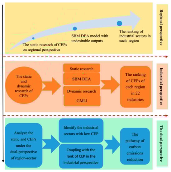
Figure 1.
Technological route map.
Then, in the industrial perspective, due to the low developed level of industry in six provinces, the top one of the six same industrial sectors might be with the lower CEP in reality. Aiming to avoid the impractical results in industrial perspective, we took Beijing as the high level of industries and Liaoning as the average level into the industrial scale research. Therefore, to solve this problem, we adopted SBM DEA model to measure the static CEPs of the same industrial sectors among eight provinces including Jilin, Heilongjiang, Inner Mongolia, Gansu, Ningxia, Xinjiang, Beijing and Liaoning from 2006 to 2015. The SBM DEA model was mainly used to measure the CEP within a cross-sectional data framework and not over time. In addition, there is no comparability for CEP in each year. Therefore, we adopted the GMLI to measure the dynamic change of CEP of the same industrial sector among eight provinces over time. To explore the driver of change of CEP, we decomposed the value of GMLI into efficiency change (EC) and best practice gap change (BPC) components. Although this, we can obtain the emission reducing potential of each industry in each region. In the industrial perspective, we can only obtain the ranking of CEPs of each province in each industry. However, it is unreasonable to evaluate the CEP without consider the different techniques and economic development levels in different regions.
Finally, from the regional perspective, the ranking of CEPs of different industrial sectors in a region is insignificant to improve the CEP without considering of industry heterogeneity. From the industrial perspective, the ranking of CEPs of the same industrial sector in different regions is unreasonable under the different techniques and economic development levels. Therefore, we analyzed the static and dynamic CEPs of the industrial sectors in six undeveloped provinces during 2006–15 periods under the dual-perspective of region-sector in the paper. Coupling with the results of CEP under regional and industrial perspective, we proposed the pathway of carbon emissions reduction in industrial scale in six provinces.
2.1. SBM DEA Model with Undesirable Output
SBM DEA Model with Undesirable Output
We assume n DMUs (decision making units), each with three factors: inputs, good (desirable) outputs, and bad (undesirable) outputs. Each unit uses m input factors to produce s1 desirable outputs and s2 undesirable outputs.
If the input and output factors are represented by three vectors: x ∈ Rm, and , then the matrices , , and can be defined respectively as follows:
The production possibility set (PPS) can be described as follows:
where is the non-negative intensity vector, thereby indicating that the above definition corresponds to the constant returns to scale (CRS) condition.
Based on the PPS and Tone’s SBM model [55], the undesirable outputs can be measured as follows:
where the vector denotes the shortage of desirable outputs, and vectors and correspond to the excesses of inputs and undesirable outputs, respectively. The subscript 0 means a DMU whose efficiency is under evaluation. The objective function has values in the range [0, 1]. For a given evaluated DMU, if and , the DMU is SBM-efficient. If , then the DMU is inefficient. Hence, it can be improved and rendered efficient by deleting the excesses in inputs and bad outputs and augmenting the shortage in desirable outputs.
In this paper, we used capital (K), labor (L), and energy (E) as the input factors, and GDP (Y) and CO2 emissions (C) as the desirable output and undesirable output, respectively.
On the basis of Equation (1), the production technology set can be defined as:
On the basis of Equations (2) and (3), the SBM DEA model to measure the CEP can be defined as [58]:
In Equation (4), is a non-negative intensity vector. Here, denotes the shortage of desirable outputs, and , , , and refer to the excess inputs of K, L, E, and the undesirable output C, respectively. The subscript “0” means a DMU whose efficiency is under evaluation. The subscript “j“ means the observation j. The observation is efficient in the presence of CO2 emissions if , thereby suggesting that .
Meanwhile, the CEP can be measured by the ratio of the target CO2 emissions to real CO2 emissions using the equation
2.2. Global Malmquist-Luenberger Index (GMLI)
The DEA model described in Equations (1)–(5) are mainly used to measure the CEP within a cross-sectional data framework and not over time. In addition, no comparability for the CEP in each year is found. For a specific DMU, the changes in the CEP over time should be tracked [24].
The GMLI was first proposed by Oh [59] as an alternative to an environmentally sensitive productivity growth index, which can estimate the dynamic change of CEP over time. Since then, the GMLI has been widely applied in different areas [60,61]. The GMLI equation is defined below.
In Equation (6), represents the directional distance function. According to Equation (3), the production technology set at period T is defined as follows:
where .
Therefore, the global production technology set is defined as follows:
where and were the efficiency values of DMUn based on its inputs, desirable outputs, and undesirable outputs at period for the reference technology at and . and are the efficiency values of DMUn based on its inputs, desirable outputs, and undesirable outputs at period for the reference technology at and . In addition, and are the efficiency values of DMUn based on its inputs, desirable outputs, and undesirable outputs at period and under the reference technology of the global production technology set.
GMLI can be used to evaluate the dynamic CEP of DMUn from period to period . , and indicate that the CEP of DMUn has gained, remained unchanged, or decreased from period to , respectively. Meanwhile, , the efficiency change term, measures change in the technical efficiencies during the two periods. and correspond to the efficiency gain and loss, respectively, and indicates the catching-up or lag with the contemporaneous benchmark technology frontier.
, the best practice gap change between the two time periods, represented the change of the technique between the two periods. , corresponded to technical progress or regress.
3. Case Study
3.1. Research Zone
The northern provinces included Jilin, Heilongjiang, Gansu, Ningxia, Inner Mongolia, and Xinjiang were chosen as the research zone in the paper, as shown in Figure 2. GDP of these provinces were lower than the national average value from 2006 to 2015. However, the carbon emissions of these provinces were higher than average level of China accordingly. Generally, the industry was the primary support of economic development in the research zone. The portion of the industry in the six provinces were all more than 40%. Therefore, the low carbon efficiency and the high industry portion were the characters of the research zone. How to control the regional carbon emissions from the industrial perspective was significant to the carbon emissions reduction in the provinces. Thus, the CEPs of 22 industrial sectors, as shown in Table 1 in the six provinces were estimated based on the regional evaluation and industrial results to propose the pathway of carbon emissions reduction in undeveloped provinces in northern China.
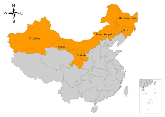
Figure 2.
The geographical location of the study area.

Table 1.
The numbers of 22 industrial sectors.
3.2. Data
In the research, we used capital, labor and energy of the industrial sectors as the input factors. GDP and CO2 emissions were adopted as the desirable output and undesirable output accordingly.
In input factors, we used the number of employees to represent labor input. The net value of fixed assets at 2006 constant price was used to indicate the capital stock. We can obtain the above data from the Statistical Yearbook of each province, China Statistical Yearbook (2007–2016) [62], China Industrial Economic Statistical Yearbook (2007–2016) [63].
In the paper, we used the total industrial terminal consumption of raw coal, coke, crude oil, gasoline, kerosene, diesel oil, fuel oil, natural gas and electricity as the energy input. The converting coefficient of standard coal in the statistical yearbook was applied to uniform the energy consumption from the different kinds of energy. We obtained the abovementioned data from the China Energy Statistical Yearbook and Statistical Yearbook of each province.
Meanwhile, we applied GDP at 2006 constant price as the desirable output in our research. According to the Intergovernmental Panel on Climate Change (IPCC) [64], we can calculate the CO2 emissions from energy consumption and corresponding carbon emission coefficients. We regarded CO2 emissions of industrial sectors as undesirable output. The original data are from the Statistical Yearbook of each province and China Statistical Yearbook. Descriptive statistics of the five basic variables are shown in Table 2.
Table 2.
Description of variables.
4. Results and Discussion
4.1. Results
4.1.1. Regional Perspective
The average CEP values during 2006–2015 in each province varied (Figure 3). However, we observed some similar characteristics of industrial sectors through the regional results. For instance, Sector 4 in three provinces had the highest CEP with the value of 1. By contrast, the CEP of Sector 21 in each province was under 0.3. Evaluations in six provinces revealed that Gansu had the highest CEP level. The lowest value of CEP in Gansu was 0.05 for Sector 13 and was higher than the lowest value of CEP in the five other provinces. Furthermore, most frontier industries were found in Gansu. Unlike Gansu, Xinjiang Province had the lowest CEP. In Xinjiang, the lowest CEP value appeared in Sector 13. Moreover, regional homogeneity was obvious in six provinces. In the northeastern provinces of Jilin and Heilongjiang, the advantageous sectors were more similar than those in the other provinces. The two provinces had CEP values of 1 for Sector 4. The disadvantageous industry in Jilin was same as that in Heilongjiang, namely, Sector 20, which was one of the sectors with low CEP. Regional homogeneity also occurred in the northwestern provinces. Sector 2 was the frontier industry with a CEP of 1 in Gansu, Ningxia, and Xinjiang.
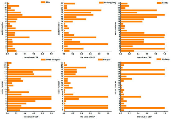
Figure 3.
The average value of carbon emission performance (CEP) of each industry in the period of 2006–15 in six provinces.
For the comprehensive analysis, the yearly CEP values of each industrial sector in the six provinces were calculated by SBM (shown in Figure 4.). The year-by-year regional results revealed an obvious transformation in each province. In Jilin, Sector 16 was always the frontier industrial sector in the whole research period. This outcome is due to the fact that the automobile industry is one of the key construction projects in the old northeastern industrial base of Jilin Province. Unlike the case of Jilin, Sector 7 in Heilongjiang was the frontier industrial sector from 2006 to 2011. However, the CEP of Sector 7 decreased to 0.4 in 2012. As a result, Sector 4 replaced Sector 7 to become the frontier industrial sector. Sector 7 involves a light industry, which has low carbon emissions. However, Sector 4, as the heavy industry, obtained a higher income based on the national economic incentive after 2012. The technical frontier industrial sectors in Jilin and Heilongjiang were both heavy industries. As the old industrial bases, the northeastern provinces had the technical advantage in enhancing the CEP of the heavy industries. Sectors 4 and 17 became the technical frontier industry at different times in Gansu. Except for Sectors 4 and 17, all other sectors were light industries with lower emissions. Thus, the heavy industry was not the dominant one in Gansu. Light industry could obtain more earnings with lower carbon emissions. The same phenomenon existed in Ningxia and Xinjiang, which had three main technical frontier industrial sectors each. For Ningxia, the pillar industry before 2012 was Sector 6, then Sector 19 became dominant in the following two years, and the highest CEP from 2012 belonged to Sector 7. Due to the huge amounts of water pollution emissions, the development of Sector 6 was constrained by the government at all levels after 2011. For Xinjiang, Sector 17 had the leading CEP from 2006 to 2011. In the following year, Sector 19 replaced Sector 17 to become the technical frontier industry. In 2012 to 2015, the CEP of Sector 22 was 1. Unlike the northeastern provinces, their counterparts in the northwestern region had no obvious advantages in the technical frontier. The condition of Inner Mongolia was similar to that of the northwestern region, namely, Sector 21 was the pillar industry before 2010. In the following years, Sectors 7 and 19 were the dominant industries. The benefit from gas production in Inner Mongolia declined with the push of the west-to-east gas transmission project. Therefore, light industry with lower emissions replaced heavy industry.
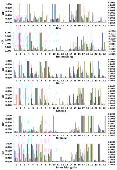
Figure 4.
The CEP of 22 industrial sectors in six provinces in the period of 2006–15.
4.1.2. Industrial Perspective
(1) Static carbon emission performance
Most of the industrial sectors in the production frontier are in Inner Mongolia (Figure 5). The percentage of industrial sectors in the production frontier in Inner Mongolia exceeded 50% of the 15 typical industrial sectors. Thus, the CEP of Inner Mongolia was superior to that of the other provinces. However, from a regional perspective, Gansu had the highest CEP. The conflict confirmed that a gap existed between the regional evaluation and the industrial results. The heterogeneity was evident in every industry assessment. For instance, the CEP of Sector 4 in Heilongjiang was in the production frontier under the industrial perspective. In the same way, the CEP of Sector 4 in Heilongjiang was also one under the regional perspective. Sector 4 was the advantageous industry in Heilongjiang. On the contrary, Sector 4 for Jilin was in the production frontier under the regional perspective, but its CEP was only 0.24 under the industrial perspective. Hence, conflicts between the regional results and the industrial evaluation exist in most industries.
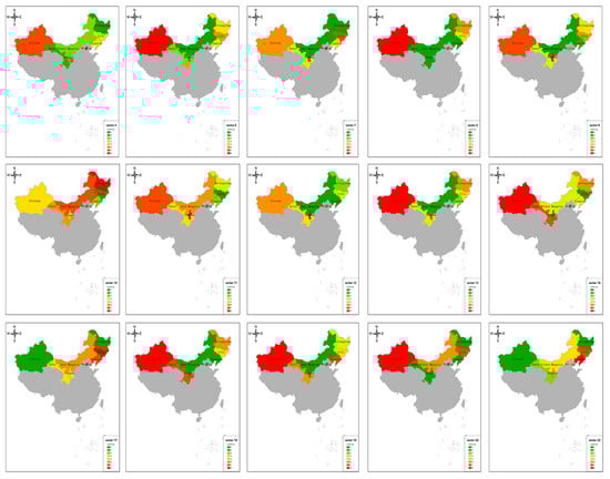
Figure 5.
The ranking of average value of CEP in eight provinces at the industrial level.
As shown as Figure 6, the annual evaluation of each industrial sector showed the transformation of the production frontier in a time series. Sector 2 in Inner Mongolia was in the production frontier after 2007 (Figure 6.). Given that Inner Mongolia was the most critical natural gas base, the technical level of Sector 2 in Inner Mongolia was the highest in eight research zones. For Sector 4, the frontier transformed from Inner Mongolia to Heilongjiang in 2011. The building material sector was the pillar industry of Heilongjiang, therefore, the technical level of Sector 4 in Heilongjiang was the highest in eight provinces. For Sector 6, the production frontier region transformed between Inner Mongolia and Ningxia. The change was caused by the high earnings due to the constraints imposed upon the small paper manufacturers. The same phenomenon occurred in Sector 7, wherein Inner Mongolia remained on the production frontier during the whole research period. Due to the higher income and lower emissions, industry transformation in Inner Mongolia occurred. For Sector 10, Liaoning and Jilin became the production frontier region at a different time. For Sector 11, most provinces were in the production frontier, including Jilin, Liaoning, Heilongjiang, Inner Mongolia, and Beijing. Spirited competition was present among the eight provinces. As for the Manufacture of Non-metallic Mineral Products (Sector 12), Inner Mongolia was always in the production frontier during the research period. For Sector 13, the CEP of Inner Mongolia was equal to unity since 2006. Conversely, Beijing was always in the production frontier except during 2008 and 2009. The relocation of steelworks in Beijing in 2008 led to the change. For Sector 16, Jilin was the production frontier region from 2006 to 2016, because the automobile industry is one of the pillar industrial sectors of Jilin Province and has advanced technology. The CEP of Inner Mongolia, Ningxia, and Beijing were on the production frontier at different times. By contrast, the CEP of Xinjiang has been the lowest during the research period, and its technology fell behind the production frontier. For the Manufacture of Electrical Machinery and Apparatus (Sector 17), the CEP of Xinjiang has been in production frontier except for 2012–2013, when it was replaced by Gansu, Inner Mongolia, and Beijing. For the Manufacture of Computers, Communication and Other Electronic Equipment (Sector 18), the CEP of Inner Mongolia was at the production frontier from 2006–14, but fell behind the production frontier in 2015 because of the massive emission of CO2. The Manufacture of Instrumentation and Cultural Office Machinery (Sector 19) of Inner Mongolia has been on the production frontier, whereas the CEP of Gansu and Jilin ranked as the lowest two, thereby indicating that the technology of these two provinces was relatively backward. For the Production and Supply of Electric Power and Heat Power (Sector 20), the CEP of Beijing has always been on the production frontier with its advanced technology and management level. Jilin performed poorly during the study period. For the Production and Supply of Water (Sector 22), the CEP of Heilongjiang was always on the production frontier except in 2015 when it was replaced by Xinjiang, thereby indicating that Xinjiang’s technology showed a trend of improvement.
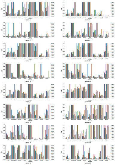
Figure 6.
The value of CEP in 8 provinces at the industrial level in the period of 2006–2015.
We note several findings from the above results. First, the level of carbon performance in Beijing is not the highest among the eight provinces. This circumstance caused the industry transformation in Beijing from the secondary industry to the third industry to be terminated. Thus, its earnings from the secondary industry was relatively lower than that of the other provinces. On the contrary, Inner Mongolia had the highest CEP. However, transformation from the heavy industry to the light industry transpired. The CEPs of heavy industries in Inner Mongolia were equal to 1 in the earlier years but were lower than 1 in recent years. Hence, the development of heavy industries in Heilongjiang and Ningxia filled the gap in the heavy industries caused by the transformation in Inner Mongolia.
(2) Dynamic carbon emission performance
As shown as Figure 7 and Figure 8, northeastern regions share a similar Sector 2. The GMLI of Inner Mongolia had a sudden increase in 2011–2012 because of the improvement of BPC. As for the average of GMLI in 2006–2015, the GMLI values of Sector 2 in all provinces exceeded 1. Thus, the CEPs of Sector 2 in these eight provinces enhanced from 2006 to 2015, among which BPC played a critical role in the improvement of CEP. For Sector 4, the GMLI of each province was equal to 1. As for Sector 6, Inner Mongolia had the highest GMLI because it has the most advanced technology relative to the other seven regions. As for Sector 7, the GMLI of Inner Mongolia suddenly decreased in 2007–2008, thereby indicating that the carbon efficiency decreased in 2008 as caused by the decrease of EC. For Sector 8, the GMLI of Inner Mongolia was under 1 only in 2008–2009, 2009–2010, and 2014–2015, an outcome which suggests that the CEP was decreasing in 2009, 2010, and 2015 because of BPC. For Sector 10, the GMLI of Jilin was under 1 from 2007–2008 and from 2010–2011, thereby indicating a decrease in CEPs in 2008 and 2011. For Sector 9, the GMLI in Inner Mongolia fluctuated significantly, with a maximum of 1.54 in 2011–2012 and a minimum of 0.87 in 2012–2013 (which was caused by BPC). For Sector 11, the GMLI in Jilin fluctuated significantly, with the maximum of 1.27 in 2009–2010 and a minimum of 0.72 in 2011–2012 (which was caused by BPC). The GMLI of Liaoning always exceeded 1 during the study period, thereby suggesting that the CEP keeps increasing during 2006–2015. For Sector 12, the GMLI of Heilongjiang fluctuated most significantly, with a maximum of 1.89 in 2011–2012 and a minimum of 0.72 in 2012–2013 (which was caused by EC). For Sector 13, the GMLI of Beijing always varied during the study period, an outcome which implies an unstable development of this industry in Beijing. For Sector 16, the GMLI of Jilin was below 1 only in 2010–2011 and 2012–2013, which can be attributed to the BPC. That result suggests that the CEP in 2011 and 2013 declined. Although the CEP of Jilin was always at the production frontier, it still tried to improve its CEP value. The most significant change in the GMLI occurred in Inner Mongolia, with a maximum of 1.59 in 2011–2012 and a minimum of 0.7 in 2012–2013 (which caused by EC). For Sector 17, the change of GMLI in each region was significant over time. For Sector 18, the GMLI in Inner Mongolia exceeded 1 during the research period except for 2011–2012 and 2014–2015, an outcome which was caused by BPC. Thus, the CEP of Inner Mongolia kept increasing during 2006–2015. Similar to the findings for Sector 17, the GMLI of Sector 19 always varied during 2006–2015. However, in terms of average GMLI, only the GMLI in Heilongjiang was below 1. EC drove the descent of CEP. For Sector 20, the CEP of Beijing was always at the production frontier during 2006–2015, but its GMLI did not always exceed 1 and was below 1 in 2007–2008, 2008–2009, and 2010–2011 because of the decline of BPC. For Sector 22, the GMLI of Heilongjiang fluctuated significantly, with a value below 1 in 2006–2009 and 2012–2015 and above 1 in 2009–2012, thereby indicating the unstable development of the sector.
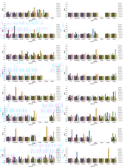
Figure 7.
Dynamic carbon emission performance of eight provinces at the industrial level, 2006–2015.
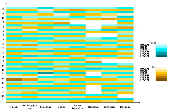
Figure 8.
The decompositions of GMLI in 8 provinces at the industrial level, 2006–2015.
In summary, most industrial sectors in the eight regions showed an ascent in carbon efficiency (Table 3). Especially in Jilin, the GMLI of all industrial sectors exceeded 1. The outcome is the same in Beijing, which achieved the top level of carbon efficiency. Backwardness was noted in only one sector in Liaoning and Xinjiang. For Inner Mongolia, the Production and Supply of Electric Power and Heat Power (Sector 20) fell behind in carbon efficiency. From the dynamic assessment, the northwestern region showed backwardness in numerous industrial sectors. The GMLI values of four industrial sectors in Ningxia and eight industrial sectors in Gansu were below 1.
Table 3.
Dynamic carbon emission performance of eight provinces at the industrial level, 2006–2015.
Compared with the result from a regional perspective, the industrial perspective indicated low ranking for some sectors with high CEP in regional results (such as Sector 17 in Jilin). Thus, considering the conflict between the two perspectives is necessary.
4.1.3. The Dual-Perspective of Region–Sector
As shown in Figure 9. for Jilin Province, the CEPs of Sector 4 ranked in the top 30%. However, at the industrial level, the CEPs of Sector 4 ranked lower. Thus, a conflict exists between the regional and the industrial perspectives. Sectors 10 and 16 were the advantageous industries that developed well from the region–sector dual perspective. On the contrary, Sector 5 did not perform well from this perspective. Thus, we should give more attention to these four industrial sectors in improving the technology level.
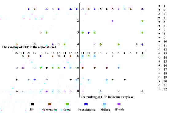
Figure 9.
Ranking of carbon emission performance under the dual-perspective of region–sector.
From the view of the region, the CEPs of Sectors 4 and 19 in Heilongjiang ranked in the top 30%. However, at the industrial level, the CEPs of these two industrial sectors ranked lower. Combined the regional and the industrial views, Sector 4 was revealed to be the advantageous industry. Sector 3 did not perform well from the region–sector dual perspective. Notably, the CEPs of Sector 20 ranked in the bottom 30% from the regional perspective but ranked first at the industrial level. Thus, this industry had no room to improve carbon efficiency at the current technical level.
From the perspective of the region, the CEPs of Sector 2 in Gansu Province ranked in the top 30%, whereas Sector 22 ranked in the bottom 30%. Results for Gansu from the industrial perspective show a different ranking in that the, CEPs of Sector 2 were below 1. In contrast to the top 30% industrial sectors, the CEP of Sector 20 was ranked top 1 at the industrial perspective. Thus, an industry with a high CEP value at the regional perspective might not develop well from the industrial perspective. In summary, Sector 8 was the advantageous industry which developed well from the region–sector dual perspective, whereas Sector 22 did not perform well from this perspective.
Coupling the regional results with the industrial results revealed that the CEPs of Sector 6 in Ningxia ranked in the top 30%. However, at the industrial level, the CEPs of Sector 6 ranked lower. Thus, the technology in Sector 6 was backward and behind the production frontier. From the dual perspective, Sector 2 represented profitable industries. On the contrary, Sector 5 did not perform well from this perspective.
From the dual perspective of the regional industrial sector, the CEP of Sector 16 in Inner Mongolia ranked in the top 30%. However, at the industrial level, the CEP of Sector 16 ranked lower. Sector 2 represented profitable industries from the region–sector dual perspective. On the contrary, the CEPs of Sectors 21 and 13 ranked in the bottom 30% but ranked first at the industrial level. Therefore, industrial sectors with low CEP values in Inner Mongolia might not develop badly compared with others.
From the regional perspective, the CEPs of Sector 2 in Xinjiang ranked in the top 30%. On the contrary, Sector 9 ranked in the bottom 30%. However, at the industrial level, the CEPs of Sector 2 ranked lower. Compared with the regional scale and the industrial level, results showed that an industry with high CEP value at the regional perspective might not develop well under the industrial perspective. Sectors 17 and 22 were the advantageous industries at the region–sector dual perspective.
Due to the varied economic development levels and industrial structures, conflicts exist between the regional and industrial results. Therefore, we examined the CEP values of the northern provinces of China under the region–sector dual perspective in this paper.
4.1.4. Uncertainty Analysis
The major sources of uncertainty exist in the carbon coefficient. In the paper, we assumed that the data of cost, labor, GDP, energy consumption in the research period were all accurate. They have no contribution on the uncertainties in research. Additionally, we assumed that the result from research by Liu et al. was correct. According to the above assumption, the carbon emissions calculated in the paper were more than exist in reality. However, the CEP assessment was the one of research targets but not carbon emissions. Meanwhile, the CEP assessment was the relative comparison. The ranking of carbon emissions was more important than the value of carbon emissions. Thus, in the premise of certain energy consumption, the different carbon coefficients only caused the different value of carbon emissions but cannot change the ranking of carbon emissions in different regions or industrial sectors. From this point, the different carbon efficient could not cause the difference in CEP results.
4.2. Discussion
In the regional perspective, different regions had the different ranking of CEPs. For example, in Jilin Province, the six sectors represent the key hindrances to enhancing the carbon efficiency of the entire province. While in Heilongjiang Province, sectors with low carbon efficiency should introduce more advanced techniques from other regions for improving their carbon efficiency. In contrast with the top 30% industries, Sectors 3 and 10 should be improved to enhance carbon efficiency. In Gansu Province, Sector 8 was the advantageous sector in Gansu Province. Different from the above provinces, the advantageous sectors were obvious in terms of CEP values. Sectors 2 and 5 were ahead of the other sectors in Inner Mongolia in carbon efficiency. In Xinjiang Autonomous Region, the bottom 30% sectors under the regional view also lag the industrial technical frontiers of the respective industries under the industrial perspective. In other words, the disadvantage in the production technique and management caused the backwardness in the carbon efficiency of Xinjiang. In Ningxia Autonomous Region, the result was the complete opposite to that for Xinjiang. Five top 30% sectors of Ningxia were found on the technical frontier.
In the industrial perspective, both Sectors 5 and Sector 22 in Jilin Province lag the industrial frontier. As the energy processing sectors, the Production and Supply of Electric Power and Heat Power (Sector 20) had the characteristic of low energy conversion. In Heilongjiang, Production and Supply of Electric Power and Heat Power (Sector 20) lowered the carbon efficiency of Heilongjiang while the sector was on the industrial frontier. In Gansu Province, the Manufacture of Textile, Wearing Apparel and Accessories, Leather, Fur, Feather and Related Products and Footwear (Sector 7) lagged in the industrial frontier. In Inner Mongolia, Sector 2 and Sector 5 were on the technical frontier along with the same sectors in all provinces. Different from Inner Mongolia, Sectors 2 and 15 were behind the industrial frontier. For Ningxia, Sectors 2 and 20 were the benchmarks of their respective sectors.
In summary, irrationality occurs in the CEP assessment under the regional or industrial perspectives. From the regional perspective, sectors with high CEP might lag the industrial technical frontier. Conversely, from the industrial perspective, the sectors on the industrial technical frontier might be the bottleneck of enhancing carbon efficiency in the research zone. Thus, the evaluation from the region–sector dual perspective was necessary. Meanwhile, the conflict between the regional and industrial results was more evident in the northeastern provinces like Jilin and Heilongjiang. The results indicated the consistency of the results under the respective views in the northwestern provinces like Xinjiang and Ningxia. The process of industrial development caused the difference. In the northeast, heavy industry was the pillar industry due to the long history of industrial development. Therefore, some sectors in the study area had high carbon intensity and advanced technology. However, during the industrial transformation, emerging industries with high carbon efficiency lacked advanced and efficient technique and management. By contrast, the northwest emphasized industries that depended on natural resource, such as mining. The long development led to a high technical level. Sectors based on such resource were the pillar industries that provided the most economic benefits. Despite the relatively late start of the other sectors with low carbon intensity, no significant advantages were observed in both technical level and economy scale.
5. Conclusions
Aiming to the gap between the CEP evaluations under the regional view and the industrial perspective accordingly, a dual-perspective coupling the regional assessment with the industrial estimation was presented in the paper. We took the northern provinces of China as a case study. The dual model of SBM DEA model and GMLI models were adopted to evaluate the static CEP and the dynamic change of CEP in research. Based on the model, we not only analyzed the CEP of 22 industrial sectors in the six regions from 2006 to 2015 but also measured the static and dynamic CEP of eight regions in 22 industrial sector from 2006 to 2015. We then identified the truly advantage and disadvantage industrial sectors in a region and propose suggestions for local policies addressing CEP improvement.
A comparison of the results under the different perspectives proved the irrationality of our evaluation under the sole perspective. For example, for Jilin Province, the CEPs of Mining and Processing of Nonmetal and Other Ores (Sector 4) ranked in top 30% in the regional perspective. However, in the industrial level, the CEPs of Mining and Processing of Nonmetal and Other Ores (Sector 4) ranked lower. The CEPs of the Production and Supply of Electric Power and Heat Power (Sector 20) of Heilongjiang Province ranked in the bottom 30% in a regional perspective but ranked first at the industrial level. We also found the advantage sectors in the CEP under the region–sector dual perspective. For example, for Jilin Province, the Processing of Petroleum, Coking, and Processing of Nuclear Fuel (Sector 10) and the manufacture of Transport Equipment (Sector 16) were the advantageous sectors. Considering the industrial transformation and the heterogeneity in the industrial process of the different regions, accelerating the development of emerging sectors was proposed as a way to enhance carbon efficiency.
Based on the above results, we put forward the following policy recommendations. First, it was inevitable to constantly promote regional economic development, especially to advocate coordinated development among northwestern China and northeastern China. Aiming at the different CEP under the region–sector perspective, northeastern and northwestern China should support regional coordinated development. Second, policy makers should focus on technology improvement and innovation and industrial structure adjustment in northeastern and northwestern China. Third, different policies and management mode should be applied for advantage and disadvantage sectors in a region. In Jilin Province, the automobile industry is one of the key construction projects in the northeast old industrial base. Therefore, the technology and management mode of Manufacture of Transport Equipment should be exported to the other provinces in the study area. On the contrary, more advanced technology in the Production and Supply of Electric Power and Heat Power with high conversion efficiency should be imported from Heilongjiang and Gansu for improving the carbon efficiency of this sector in Jilin, while in Heilongjiang, Mining and Processing of Nonmetal and Other Ores and Manufacture of General and Special Purpose Machinery were the benchmarking in the dual perspectives. Thus, the production technology and management mode in the two sectors could provide a development reference for the same sectors in other provinces. For Gansu, the conflict between the regional results and the industrial results was more evident. From the industrial perspective, there were no industrial sectors on the frontier. Meanwhile, the industrial sectors with higher CEP in regional results have the low carbon efficient, such as Manufacture of Textile, Wearing Apparel and Accessories, Leather, Fur, Feather and Related Products and Footwear, lagged behind those of the other sectors. Therefore, Sector 7 should consider the importation of the technique and management from Heilongjiang and Ningxia. For Inner Mongolia, Sectors 2 and 5 were ahead of the other sectors in Inner Mongolia in carbon efficiency. From the industrial scale, the above were on the technical frontier along with the same sectors in all provinces. Therefore, developing the two sectors is an effective way to reduce carbon emissions in Inner Mongolia. In Xinjiang, Sectors 2 and 15 were behind the industrial frontier, although the four sectors lead in terms of CEP values from the regional results. The dual perspective results indicate that the four relatively advanced sectors should improve their technique and management to be close to the frontier. For Ningxia, Sectors 2 and 20 were the benchmarks of their respective sectors. For reducing carbon emissions, we should focus on the development of these two sectors.
No fixed production frontier was available in DEA method. The unconditional advanced sectors could not be obtained from DEA. Thus, comparison between the regional results and the industrial results must be introduced. In our future work, the fixed production frontier like SFA may be introduced quantitatively into efficiency assessment for the more reasonable rank of different regions and sectors. In addition, with the status of different sectors in six northern provinces representing the production frontier, the uncertainty in the assessment exists in the study. The relationship between the carbon emissions and the carbon efficiency was not discussed in our research, but it will be tackled in our next work.
Author Contributions
Conceptualization, X.W. (Xian’En Wang) and S.W. (Shimeng Wang); methodology, X.W. (Xian’En Wang); software, S.W. (Shimeng Wang); validation, W.L., J.S. and H.D.; formal analysis, S.W. (Shuo Wang); investigation, W.L., J.S. and H.D.; resources, X.W. (Xipan Wang); data curation, X.W. (Xipan Wang); writing—original draft preparation, S.W. (Shimeng Wang); writing—review and editing, S.W. (Shuo Wang); visualization, J.S.; supervision, H.D.; project administration, S.W. (Shuo Wang); funding acquisition, X.W. (Xian’En Wang).
Funding
This research was funded by Major Projects of the National Social Science, grant number 15ZDA015.
Conflicts of Interest
The authors declare no conflict of interest.
References
- Zhang, Y.-J.; Hao, J.-F.; Song, J. The CO2 emission efficiency, reduction potential and spatial clustering in China’s industry: Evidence from the regional level. Appl. Energy 2016, 174, 213–223. [Google Scholar] [CrossRef]
- Kounetas, K. Heterogeneous technologies, strategic groups and environmental efficiency technology gaps for European countries. Energy Policy 2015, 83, 277–287. [Google Scholar] [CrossRef]
- Juudit, O.; Jukka, H.; Seppo, J. New Energy Efficient Housing Has Reduced Carbon Footprints in Outer but Not in Inner Urban Areas. Environ. Sci. Technol. 2015, 49, 9574–9583. [Google Scholar]
- Wang, K.; Yu, S.; Zhang, W. China’s regional energy and environmental efficiency: A DEA window analysis based dynamic evaluation. Math. Comput. Model. 2013, 58, 1117–1127. [Google Scholar] [CrossRef]
- Li, Y.; Sun, L.; Feng, T.; Zhu, C. How to reduce energy intensity in China: A regional comparison perspective. Energy Policy 2013, 61, 513–522. [Google Scholar] [CrossRef]
- Yan, D.; Lei, Y.; Li, L.; Song, W. Carbon emission efficiency and spatial clustering analyses in China’s thermal power industry: Evidence from the provincial level. J. Clean. Prod. 2017, 156, 518–527. [Google Scholar] [CrossRef]
- Yao, X.; Zhou, H.; Zhang, A.; Li, A. Regional energy efficiency, carbon emission performance and technology gaps in China: A meta-frontier non-radial directional distance function analysis. Energy Policy 2015, 84, 142–154. [Google Scholar] [CrossRef]
- Wang, Q.; Chiu, Y.H.; Chiu, C.R. Non-radial metafrontier approach to identify carbon emission performance and intensity. Renew. Sustain. Energy Rev. 2017, 69, 664–672. [Google Scholar] [CrossRef]
- Liu, Y.; Zhao, G.; Zhao, Y. An analysis of Chinese provincial carbon dioxide emission efficiencies based on energy consumption structure. Energy Policy 2016, 96, 524–533. [Google Scholar] [CrossRef]
- Shan, Y.; Liu, J.; Liu, Z.; Xu, X.; Shao, S.; Wang, P.; Guan, D. New provincial CO2 emission inventories in China based on apparent energy consumption data and updated emission factors. Appl. Energy 2016, 184, 742–750. [Google Scholar] [CrossRef]
- Chen, S.; Golley, J. ‘Green’ productivity growth in China’s industrial economy. Energy Econ. 2014, 44, 89–98. [Google Scholar] [CrossRef]
- Xin, Y.; Guo, C.; Shuai, S.; Jiang, Z. Total-factor CO2 emission performance of China’s provincial industrial sector: A meta-frontier non-radial Malmquist index approach. Appl. Energy 2016, 184, S0306261916311515. [Google Scholar]
- Sun, J.W. The decrease of CO2 emission intensity is decarbonization at national and global levels. Energy Policy 2005, 33, 975–978. [Google Scholar] [CrossRef]
- Zhu, Z.S.; Liao, H.; Cao, H.S.; Wang, L.; Wei, Y.M.; Yan, J. The differences of carbon intensity reduction rate across 89 countries in recent three decades. Appl. Energy 2014, 113, 808–815. [Google Scholar] [CrossRef]
- Cheng, Z.; Li, L.; Liu, J. Industrial structure, technical progress and carbon intensity in China’s provinces. Renew. Sustain. Energy Rev. 2017, 81. [Google Scholar] [CrossRef]
- Lee, C.-C.; Chang, C.-P. Stochastic convergence of per capita carbon dioxide emissions and multiple structural breaks in OECD countries. Econ. Model. 2009, 26, 1375–1381. [Google Scholar] [CrossRef]
- Jobert, T.; Karanfil, F.; Tykhonenko, A. Convergence of per capita carbon dioxide emissions in the EU: Legend or reality? Energy Econ. 2010, 32, 1364–1373. [Google Scholar] [CrossRef]
- Lin, B.; Li, X. The effect of carbon tax on per capita CO2 emissions. Energy Policy 2011, 39, 5137–5146. [Google Scholar] [CrossRef]
- Lu, M.; Wang, X.; Cang, Y. Carbon Productivity: Findings from Industry Case Studies in Beijing. Energies 2018, 11, 2796. [Google Scholar] [CrossRef]
- Hu, X.; Liu, C. Carbon productivity: A case study in the Australian construction industry. J. Clean. Prod. 2016, 112, 2354–2362. [Google Scholar] [CrossRef]
- Wang, Q.; Zhao, Z.; Peng, Z.; Zhou, D. Energy efficiency and production technology heterogeneity in China: A meta-frontier DEA approach. Econ. Model. 2013, 35, 283–289. [Google Scholar] [CrossRef]
- Lin, B.; Du, K. Modeling the dynamics of carbon emission performance in China: A parametric Malmquist index approach. Energy Econ. 2015, 49, 550–557. [Google Scholar] [CrossRef]
- Wang, C.; Zhan, J.; Bai, Y.; Chu, X.; Zhang, F. Measuring carbon emission performance of industrial sectors in the Beijing-Tianjin-Hebei region, China: A stochastic frontier approach. Sci. Total Environ. 2019, 685, 786–794. [Google Scholar] [CrossRef] [PubMed]
- Zhou, P.; Ang, B.W.; Han, J.Y. Total factor carbon emission performance: A Malmquist index analysis. Energy Econ. 2010, 32, 194–201. [Google Scholar] [CrossRef]
- Herrala, R.; Goel, R.K. Global CO2 efficiency: Country-wise estimates using a stochastic cost frontier. Energy Policy 2012, 45, 762–770. [Google Scholar] [CrossRef]
- Dong, F.; Li, X.; Long, R.; Liu, X. Regional carbon emission performance in China according to a stochastic frontier model. Renew. Sustain. Energy Rev. 2013, 28, 525–530. [Google Scholar] [CrossRef]
- Andor, M.; Sommer, S.; Parmeter, C. Combining Uncertainty with Uncertainty to Get Certainty? Efficiency Analysis for Regulation Purposes. Eur. J. Oper. Res. 2019, 274, 240–252. [Google Scholar] [CrossRef]
- Kao, C. Network data envelopment analysis: A review. Eur. J. Oper. Res. 2014, 239, 1–16. [Google Scholar] [CrossRef]
- Thijssen, G.J. Environmental efficiency with multiple environmentally detrimental variables; estimated with SFA and DEA. Eur. J. Oper. Res. 2000, 121, 287–303. [Google Scholar]
- Zhao, L.; Zha, Y.; Zhuang, Y.; Liang, L. Data envelopment analysis for sustainability evaluation in China: Tackling the economic, environmental, and social dimensions. Eur. J. Oper. Res. 2019, 275, 1083–1095. [Google Scholar] [CrossRef]
- Wang, L.; Chen, Z.; Ma, D.; Zhao, P. Measuring Carbon Emissions Performance in 123 Countries: Application of Minimum Distance to the Strong Efficiency Frontier Analysis. Sustainability 2013, 5, 5319–5332. [Google Scholar] [CrossRef]
- Wang, Q.; Su, B.; Zhou, P.; Chiu, C.-R. Measuring total-factor CO2 emission performance and technology gaps using a non-radial directional distance function: A modified approach. Energy Econ. 2016, 56, 475–482. [Google Scholar] [CrossRef]
- Wang, Q.W.; Zhou, P.; Zhou, D.Q. Research on Dynamic Carbon Dioxide Emissions Performance, Regional Disparity and Affecting Factors in China. China Ind. Econ. 2010, 33, 45–54. [Google Scholar]
- Lin, B.; Du, K. Energy and CO2 emissions performance in China’s regional economies: Do market-oriented reforms matter? Energy Policy 2015, 78, 113–124. [Google Scholar] [CrossRef]
- Zhong, J. Biased Technical Change, Factor Substitution, and Carbon Emissions Efficiency in China. Sustainability 2019, 11, 955. [Google Scholar] [CrossRef]
- Wang, S.; Wang, H.; Zhang, L.; Dang, J. Provincial Carbon Emissions Efficiency and Its Influencing Factors in China. Sustainability 2019, 11, 2355. [Google Scholar] [CrossRef]
- Zhou, Z.; Liu, C.; Zeng, X.; Jiang, Y.; Liu, W. Carbon emission performance evaluation and allocation in Chinese cities. J. Clean. Prod. 2018, 172, 1254–1272. [Google Scholar] [CrossRef]
- Fei, R.; Lin, B. The integrated efficiency of inputs–outputs and energy—CO2 emissions performance of China’s agricultural sector. Renew. Sustain. Energy Rev. 2017, 75, 668–676. [Google Scholar] [CrossRef]
- Hu, X.; Si, T.; Liu, C. Total factor carbon emission performance measurement and development. J. Clean. Prod. 2017, 142, 2804–2815. [Google Scholar] [CrossRef]
- Ning, Z.; Xiao, W. Dynamic total factor carbon emissions performance changes in the Chinese transportation industry. Appl. Energy 2015, 146, 409–420. [Google Scholar]
- Ning, Z.; Peng, Z.; Kung, C.C. Total-factor carbon emission performance of the Chinese transportation industry: A bootstrapped non-radial Malmquist index analysis. Renew. Sustain. Energy Rev. 2015, 41, 584–593. [Google Scholar]
- Yang, J.; Tang, L.; Mi, Z.; Liu, S.; Li, L.; Zheng, J. Carbon emissions performance in logistics at the city level. J. Clean. Prod. 2019, 231, 1258–1266. [Google Scholar] [CrossRef]
- Cheng, Z.; Li, L.; Liu, J.; Zhang, H. Total-factor carbon emission efficiency of China’s provincial industrial sector and its dynamic evolution. Renew. Sustain. Energy Rev. 2018, 94, 330–339. [Google Scholar] [CrossRef]
- Lee, M.; Zhang, N. Technical efficiency, shadow price of carbon dioxide emissions, and substitutability for energy in the Chinese manufacturing industries. Energy Econ. 2012, 34, 1492–1497. [Google Scholar] [CrossRef]
- Zhang, N.; Choi, Y. Total-factor carbon emission performance of fossil fuel power plants in China: A metafrontier non-radial Malmquist index analysis. Energy Econ. 2013, 40, 549–559. [Google Scholar] [CrossRef]
- Zhang, N.; Choi, Y. A comparative study of dynamic changes in CO2 emission performance of fossil fuel power plants in China and Korea. Energy Policy 2013, 62, 324–332. [Google Scholar] [CrossRef]
- Lin, B.; Chen, X. Evaluating the CO2 Performance of China’s Non-ferrous Metals Industry: A Total Factor Meta-frontier Malmquist Index Perspective. J. Clean. Prod. 2019, 209, 1061–1077. [Google Scholar] [CrossRef]
- Lin, B.; Tan, R. China’s CO2 emissions of a critical sector: Evidence from energy intensive industries. J. Clean. Prod. 2017, 142, 4270–4281. [Google Scholar] [CrossRef]
- Wu, F.; Fan, L.W.; Zhou, P.; Zhou, D.Q. Industrial energy efficiency with CO2 emissions in China: A nonparametric analysis. Energy Policy 2012, 49, 164–172. [Google Scholar] [CrossRef]
- Cheng, Z.; Shi, X. Can Industrial Structural Adjustment Improve the Total-Factor Carbon Emission Performance in China? Int. J. Environ. Res. Public Health 2018, 15, 2291. [Google Scholar] [CrossRef]
- Xie, B.-C.; Duan, N.; Wang, Y.-S. Environmental efficiency and abatement cost of China’s industrial sectors based on a three-stage data envelopment analysis. J. Clean. Prod. 2017, 153, 626–636. [Google Scholar] [CrossRef]
- Zhang, N.; Wang, B.; Liu, Z. Carbon emissions dynamics, efficiency gains, and technological innovation in China’s industrial sectors. Energy 2016, 99, 10–19. [Google Scholar] [CrossRef]
- Yu, S.; Hu, X.; Fan, J.-L.; Cheng, J. Convergence of carbon emissions intensity across Chinese industrial sectors. J. Clean. Prod. 2018, 194, 179–192. [Google Scholar] [CrossRef]
- Wang, Y.; Duan, F.; Ma, X.; He, L. Carbon emissions efficiency in China: Key facts from regional and industrial sector. J. Clean. Prod. 2019, 206, 850–869. [Google Scholar] [CrossRef]
- Tone, K. A slacks-based measure of efficiency in data envelopment analysis. Eur. J. Oper. Res. 2001, 130, 498–509. [Google Scholar] [CrossRef]
- Chang, Y.T.; Zhang, N.; Danao, D.; Zhang, N. Environmental efficiency analysis of transportation system in China: A non-radial DEA approach. Energy Policy 2013, 58, 277–283. [Google Scholar] [CrossRef]
- Zhou, P.; Ang, B.W.; Poh, K.L. Slacks-based efficiency measures for modeling environmental performance. Ecol. Econ. 2007, 60, 111–118. [Google Scholar] [CrossRef]
- Choi, Y.; Ning, Z.; Zhou, P. Efficiency and abatement costs of energy-related CO2 emissions in China: A slacks-based efficiency measure. Appl. Energy 2012, 98, 198–208. [Google Scholar] [CrossRef]
- Oh, D.H. A global Malmquist-Luenberger productivity index. J. Prod. Anal. 2010, 34, 183–197. [Google Scholar] [CrossRef]
- Xia, K.; Guo, J.-K.; Han, Z.-L.; Dong, M.-R.; Xu, Y. Analysis of the scientific and technological innovation efficiency and regional differences of the land–sea coordination in China’s coastal areas. Ocean Coast. Manag. 2019, 172, 157–165. [Google Scholar]
- Qin, X.; Wang, X.; Xu, Y.; Wei, Y. Exploring Driving Forces of Green Growth: Empirical Analysis on China’s Iron and Steel Industry. Sustainability 2019, 11, 1122. [Google Scholar] [CrossRef]
- National Bureau of Statistics of China (NBSC). China Statistical Yearboo; China Statistics Press: Beijing, China, 2007–2016.
- National Bureau of Statistics of China (NBSC). China Industrial Economic Statistical Yearbook; China Statistics Press: Beijing, China, 2007–2016.
- IPCC. IPCC Guidelines for National Greenhouse Gas Inventories. 2006. Available online: https://www.ipcc-nggip.iges.or.jp/public/2006gl/ (accessed on 30 October 2018).
© 2019 by the authors. Licensee MDPI, Basel, Switzerland. This article is an open access article distributed under the terms and conditions of the Creative Commons Attribution (CC BY) license (http://creativecommons.org/licenses/by/4.0/).