Driver Behavior Models for Heavy Vehicles and Passenger Cars at a Work Zone

Abstract

Traffic impact assessment is a key step in the process of work zone planning and scheduling for transportation agencies. Microscopic traffic simulation models enable transportation agencies to conduct detailed analyses of work zone mobility performance measures during the planning and scheduling process. However, traffic simulation results are valid only when the simulation model is calibrated to replicate driver behavior that is observed in the field. Few studies have provided guidance on the calibration of traffic simulation models at work zones and have offered driver behavior parameters that reproduce capacity values that are observed in the field. This paper contributes to existing knowledge of work zone simulation by providing separate driver behavior model parameters for heavy vehicles and passenger vehicles. The driver behavior parameters replicate the flow and speed at the work zone taper and at roadway segments upstream of the work zone. A particle swarm optimization framework is proposed to improve the efficiency of the calibration process. The desired time headway was found to be 2.31 seconds for heavy vehicles and 1.53 seconds for passenger cars. The longitudinal following threshold was found to be 17.64 meters for heavy vehicles and 11.70 meters for passenger cars. The proposed parameters were tested against field data that had not previously been used in the calibration of driver behavior models. The average absolute relative error for flow rate at the taper was 10% and the mean absolute error was 54 veh/h/ln. The GEH statistic for the validation dataset was 1.48.

1. Introduction

Work zones intrinsically reduce roadway capacity and contribute to travel delay and congestion on urban and rural roadways [1]. Therefore, transportation agencies assess mobility and safety impacts of work zones when designing and planning roadway projects and seek to mitigate such impacts on both road users and nonusers. A traffic impact study is often conducted and measures of effectiveness, such as travel delay and length of the queue at a work zone, are estimated and taken into account in the development of work zone transportation management plans. In general, work zone traffic impact assessment techniques can be classified into two broad categories: analytical methods and traffic simulation models. Analytical methods employ queuing theory [2] and parametric and non-parametric models [3,4] to estimate work zone performance measures. These methods are coded into custom spreadsheets or are developed as standalone work zone-specific analytical tools. These tools are often computationally efficient and do not demand substantial efforts to code the work zone. The Missouri Department of Transportation’s work zone impact analysis spreadsheet, QuickZone, CA4PRS, and FreeVal-WZ are examples of such tools.

Traffic simulation models, on the other hand, are often computationally intensive and require more effort to code the work zone. However, a simulation model provides a detailed analysis of the impact of a work zone on corridor mobility and traffic operations at upstream on-ramps, off-ramps, and detour routes. A traffic simulation model also allows for the study of complex and nonconventional work zone configurations. The application of work zone traffic simulations is not limited to the development of work zone transportation management plans. Traffic simulation models are also used to develop and evaluate a work zone variable speed limit algorithm [5], assess the impact of connected vehicles on work zone safety [6], and evaluate merging strategies for work zones [7]. It is worth mentioning that traffic simulation results are only valid when the model is calibrated to replicate traffic patterns that are observed in the field; the Federal Highway Administration (FHWA) traffic analysis toolbox [8] and other researchers [9,10,11,12,13] have provided general guidelines for such calibration of traffic simulation models. However, few studies have offered specific guidance on the development and calibration of work zone simulation models [14,15]. The research that is described in this paper makes the following contributions to the existing body of knowledge on work zone traffic simulation.

First, previous research [16,17] indicates that heavy vehicle and passenger car headways at work zones follow different statistical distributions, suggesting that the driver behavior models of heavy vehicle and passenger car drivers in work zones are different. This paper investigates this hypothesis and offers driver behavior parameters for passenger cars and heavy vehicles in a work zone. To the best of the authors’ knowledge, this is the first time that heavy vehicle driver behavior models have been provided for work zones.

Second, driver behavior models are calibrated with two goals in mind: (1) to replicate capacity at work zone taper, and (2) to replicate traffic conditions upstream of the work zone. The goal is to ensure that measures of effectiveness (MOEs) that are obtained from simulation models replicate the MOEs that would occur at the work zone site.

Third, this paper proposes a framework based on the particle swarm optimization (PSO) algorithm to calibrate car-following and lane-changing model parameters in a work zone. In the calibration process, the feasible region of driver behavior model parameters is searched to find the set of parameters that replicates traffic conditions that are observed in the field. The objective of the PSO framework is to increase the efficiency of the search for a solution while ensuring that the final solution represents drivers’ behavior. The proposed framework is applicable to the calibration of driver behavior at any transportation facility.

This paper is organized as follows: first, a brief overview of the Wiedemann 99 [18] driver behavior model is provided. Second, literature on the calibration of work zone traffic simulation models is reviewed and summarized. Section three outlines the proposed framework for the calibration of driver behavior models. Section four presents results of the application of the proposed framework to a work zone on Interstate 44 in St. Louis, Missouri, in the United States. Section five summarizes the findings of the research and provides recommendations for future research.

Wiedemann 99 Driver Behavior Model

Rainer Wiedemann proposed two car-following models that were developed based on psycho-physical aspects of driving behaviors [18]. The first model is referred to as Wiedemann 74, which represents driver behavior on urban arterials. The second model is referred to as Wiedemann 99 and represents driver behavior on freeways. The Wiedemann 99 model consists of 10 parameters, which are listed in

Table 1. Wiedemann 99 car-following model parameters.

Parameter	Default Value	Description
CC0	1.50 m	Average standstill distance between two vehicles.
CC1	0.90 s	Desired headway time between lead and following vehicles.
CC2	4.00 m	Additional distance over the desired safety distance. At this stage, the driver recognizes a preceding slower vehicle.
CC3	−8.00 s	The time in seconds before a vehicle starts decelerating to the safety distance.
CC4	−0.35	Negative speed variation between lead and following vehicles. Low values result in a more sensitive driver reaction to the acceleration or deceleration of the preceding vehicle.
CC5	0.35	Positive speed variation between lead and following vehicles. Value is the positive number corresponding to the negative value of CC4.
CC6	11.44	Influence of distance on speed oscillation. Large values lead to a greater speed oscillation with increasing distance.
CC7	0.25 m/s2	Oscillation during acceleration.
CC8	3.50 m/s2	Desired acceleration from standstill.
CC9	1.50 m/s2	Desired acceleration at 80.45 km/h.

. The descriptions and default values of the Wiedemann 99 model are also reported in Table 1. The Wiedemann 99 model is implemented in VISSIM traffic simulation software. However, it is the responsibility of the software user to determine the driving behavior model parameters to represent driver behavior in any transportation facility and geographical area. Lane change (LC) distance is another parameter in VISSIM that affects the behavior of drivers. Lane change distance represents the earliest distance upstream of a link at which drivers start looking for opportunities to change a lane so that they will be in their desired lane before arriving at the destination link. The default LC value in VISSIM is 200 meters [18].

2. Literature Review

This section reviews literature that is associated with the calibration of VISSIM simulation models of uninterrupted flow facilities. The literature review is split into three categories: first, methods for calibrating simulations containing freeways without the presence of work zones are presented. The second section highlights research methods for calibrating simulations that include work zones and lane closures. The third section provides an overview of the application of PSO to solve various optimization problems.

Woody [9] outlined a process for calibration of freeway facility models in VISSIM. Suggested measures of effectiveness (MOE) for comparing simulated values to field values were travel time, vehicle speed, and queue length. Woody also performed a sensitivity analysis on driver behavior parameters to determine the effect of each parameter on the model’s performance. A one-lane conceptual model was coded and used to conduct the sensitivity analysis. Four simulation scenarios were developed for each of the 10 car-following parameters. When testing a specific parameter, all other parameters were kept at default values and the maximum flow rate was then collected from VISSIM based on 10 simulation runs. The sensitivity analysis showed that the most influential parameters on maximum observed volumes were headway (CC1), following variation (CC2), and oscillation acceleration (CC7).

Dong et al., [10] calibrated driver behavior parameters for urban freeways across the state of Iowa. Standstill distances were obtained from manual processing of videos and vehicle headway values were obtained from radar detectors. Analysis of default Wiedemann 99 model parameters indicated that the default values do not represent the driver behavior that is observed in the field. A range of possible values for driver behavior parameters was determined and multiple simulation scenarios were developed and examined. T-tests and GEH statistics were used to identify the best set of driver behavior parameters.

Gomes et al., [11] presented a method for calibrating simulation models of a congested freeway in Pasadena, California. Several combinations of CC0, CC1, and the pair of speed variation parameters, CC4/CC5, were investigated. Measures of effectiveness such as travel time and vehicle count were not used in the calibration process due to a lack of computing power and time restrictions, and the authors relied on visual identification of bottlenecks and queue characteristics, such as queue length, to identify the best set of CC0, CC1, and CC4/CC5 values.

Yeom et al., [14] created a guide for calibrating freeway work zone models by investigating several work zone scenarios with various lane configurations. The queue discharge rates (QDR) that were obtained from the simulation model and were observed from the field were used to evaluate sets of driver behavior parameters. The authors tested an extensive combination of possible values for driving behavior parameters to determine which parameters affect work zone capacity the most. The results showed that CC1 and CC2 were the two driver behavior parameters in the Wiedemann 99 model that were pivotal in replicating the work zones in the simulation model. The values of CC1 and CC2 depended on the work zone lane configuration. The author also suggested that a lane change distance value that is five times the default lane change distance value of VISSIM should be used in work zone simulation models.

Kan et al., [15] developed a VISSIM calibration model for replicating time-dependent capacity, speed, and queue length for a 2-to-1 freeway work zone with a 72 km/h speed limit. To calibrate their model, 10 replications were run for each CC0 (standstill distance) and CC1 value; that is, for finding CC1, replications were run for a fixed CC0 value while CC1 was increased by increments of 0.5 s. Likewise, for finding CC0, CC1 was fixed while CC0 values were increased by 0.76 m increments. Paired t-tests were then used to compare field data with the model, and the authors found that the optimal range for CC1 values is between 1.5 and 2.4 seconds, with numbers outside this range resulting in significantly different speed data. Also, p-values indicated that high CC1 values must be paired with lower CC0 values, and vice versa.

Weng et al., [16] suggested classifying different vehicle headway distributions near work zones into four follower–leader relationships: car–car, car–truck, truck–car, and truck–truck. Field headways were observed and estimated for peak and non-peak hours on two work zone sites in Singapore using a video camera. Using the maximum likelihood estimation and Kolmogorov-Smirnov tests, results concluded that the inverse Gaussian distribution worked best for truck–car and truck–truck relationships, while the lognormal distribution was more suitable for car–car and car–truck relationships. Headway observations also suggested that trucks maintain a higher headway than cars.

Similarly, Kong and Guo [17] investigated the interaction between cars and trucks in the Jiangsu Province of China to determine if different vehicle types observed different headway values. Using six common distribution models, they found that for freeways with flow rates from 2055 to 4333 veh/h, car–truck interactions resulted in higher headway times than car–car interactions, signifying a need for separate headway values for cars and trucks. Their results showed that the lognormal model is more appropriate for car–car and truck–truck classifications, while the inverse Gaussian model fits the car–truck and truck–car headway type.

Park and Schneeberger [19] outlined a step-by-step process for calibrating a VISSIM model for a coordinated actuated signal system of intersections along an arterial road in Virginia. Their procedure consisted of creating a simulation model, evaluating default parameter results, experimenting and running simulations with several parameter adjustments, conducting a feasibility test, performing parameter calibration using genetic algorithm (GA), evaluating results with statistical analysis, and then validating the model. A similar calibration technique was then demonstrated by Park and Qi [20] with two case studies: one involving another actuated signalized intersection and another involving a freeway work zone using four days’ worth of traffic data for an 8 km freeway segment featuring a work zone lane closure in Virginia.

In both studies, the analysis of variance (ANOVA) test was used to find the effect that several calibration parameters had on the travel time, which was the measure of effectiveness. The fitness value was defined as the difference between the average travel time from the field and from the simulation, divided by the average travel time from the field. For the intersection, the average travel time that was determined in the simulation using default parameter values was 23.4 s, which was significantly less than the field value of 56.75 s. The Latin Hypercube Sampling method was used to generate 200 scenarios with five random seeded runs for each scenario, which aided in determining desired speed distribution and minimum gap time (both p-value = 0.0) as the more important calibration parameters. A t-test was conducted to compare the GA-based results with those from the default parameter sets and the best-guess parameter sets based on the engineers’ judgment. The GA-based set produced an average travel time of 50.33 s—similar to the field results—while the latter two sets produced travel times of 23.40 s and 29.53 s, respectively.

Tettamanti and Varga [21] highlighted the importance of mathematical optimization software during the development and validation stages of traffic control measures. They introduced a VISSIM-MATLAB environment that resulted from collecting the most important properties from VISSIM COM (Component Object Model) and VISSIM API (Application Package Interface). Tettamanti et al., [22] expanded on this integrated environment by suggesting a calibration method based on a GA algorithm to accurately reflect traffic conditions. The variation of the fitness function was plotted over time, illustrating the maximum relative error that was obtained during the calibration process. The error was the difference between the link speed based on the calibrated parameters and the real-world mean speed. The resulting fitness function always remained under 22% and was considered accurate enough for calibration purposes. The desired speed distribution was created based on the free flow speeds that were obtained from the traffic sensors in the field.

Chen et al., [23] calibrated the Wiedemann 99 car-following model parameters for 10 weather scenarios by connecting a real world driving simulator with VISSIM traffic simulation software. Traffic data that were collected during a 90 min period were used to create the baseline simulation model during ideal weather conditions. Weather-related events were created in the driving simulator and were compared to baseline scenario to determine the effect of weather on roadway capacity.

The PSO algorithm is an optimization method that is inspired by the behavior of flocks of birds [24]. Deng et al., [25] utilized the PSO algorithm to solve a bi-level optimization problem involving plug-in electric vehicles (PEVs) and their impact on electricity distribution networks and on electricity price. The upper-level objective function considered the cost of obtaining energy from the grid, of energy losses in the network, and of purchasing electricity from distributed generators. The lower-level model objective function considered the charging schedule of PEVs. Dai et al., [26] proposed a method that combined multi-agent systems with the PSO algorithm to optimize the design of an integrated system of PEV charging stations and a battery energy storage system. Malik and Kim [27] utilized the PSO algorithm and neural networks to develop a combined destination and route choice model for recreational trips. The proposed method took into account travelers’ preferences, travel distance, traffic congestion, weather conditions, and the utility of the recreational sites and their constraints to suggest a destination and a route for visiting that destination. Zhao et al., [28] proposed a multi-objective hierarchical model to solve a shelter location-allocation problem. The model optimized the location of immediate shelters, short-term shelters, and long-term shelters. The PSO algorithm was utilized to determine the optimum location of shelters on the basis of minimizing the distance between evacuees and shelters.

Differentiation from Previous Literature

This paper distinguishes itself from the aforementioned literature in the following ways: first, to the best of the authors’ knowledge, this is the first paper to propose driver behavior model parameters for heavy vehicles at a work zone. The previous driver behavior studies have not studied heavy vehicles driver behavior parameters at work zones and provided one set of driver behavior models for various vehicle types in work zones. This paper presents two sets of separate driver behavior model parameters for passenger cars and heavy vehicles at work zones.

Second, the objective of the calibration of driver behavior parameters in previous studies was to replicate work zone capacity at the work area or at the taper. These studies did not take into account the upstream traffic conditions in the calibration process. In other words, the calibration process was not sensitive to queue spillbacks upstream of the work zone. This paper calibrates the simulation model to replicate traffic flow at a work zone taper and a 3 km long segment upstream of the taper. The goal of this paper is to derive behavior parameters that replicate capacity at taper and replicate traffic conditions upstream of the work zone, such as length of queue and travel time at the work zone.

Third, a framework based on the PSO algorithm is proposed to calibrate the driver behavior parameters. The PSO algorithm is expected to improve the computational efficiency of the calibration process. To the best of the authors’ knowledge, this is the first paper to investigate the PSO algorithm for the calibration of driver behavior model parameters. Particle swarm optimization is used to develop train timetables [29], optimize the structure of short-term traffic flow prediction models [30], optimize traveler information systems [31], and to optimize the vertical alignment of roadways to reduce travel time, fuel consumption, and costs associated with the maintenance of pavements [32].

Fourth, data collected during 3 days of the work zone are used to calibrate the driver behavior parameters, and data from 10 days are used to evaluate the calibration model. The evaluation data was not used in the calibration process. To the best of the authors’ knowledge, this is the first time that driver behavior parameters that were obtained from the calibration process have been validated.

3. Framework for Determining Driver Behavior Parameters

The goal of this research is to propose a set of driver behavior model parameters that produce traffic patterns in the simulation model that are similar to the traffic conditions that are observed in the field. The field data that were used in this paper for determining driver behavior parameters were collected in a long-term work zone in St. Louis, Missouri, in the United States. More information regarding the work zone configuration and data collection methods is provided in Section 4: Case Study. It is worth mentioning that the framework that is proposed in this paper is applicable to various roadway facilities, such as arterials and roundabouts, and is not limited to work zones.

Previous work zone driver behavior model calibration studies are similar in that they all agree that desired time headway (CC1) and longitudinal following threshold (CC2) are the parameters that should be calibrated [9,14,31]. Introducing a second vehicle class (i.e., trucks) to the calibration process doubles the size of the solution region or search space for optimal driver behavior parameters, and there is a trade-off between the dimension of search space and the time required to identify optimal solutions. Thus, this paper focuses on the calibration of desired time headway for passenger cars ($CC{1}_P$) and for heavy vehicles ($CC{1}_T$), as well as longitudinal following threshold for passenger cars ($CC{2}_P$) and for heavy vehicles ($CC{2}_T$). Lane change ($LC$) distance is another parameter that is shown to affect lane-changing behaviors in traffic simulation models. However, this value is the same for all vehicle classes in VISSIM and cannot be calibrated separately for different vehicle classes. Therefore, this paper is searching for driver behavior parameters for passenger cars and heavy vehicles (i.e., desired time headway, longitudinal following threshold, and lane change distance) that minimize dissimilarities between traffic simulation data and ground truth data. This objective is presented in Equation (1).

$$minimize f\left(\mathit{x}\right), \mathit{x}=\left(CC{1}_P,CC{2}_P,CC{1}_T,CC{2}_T, LC\right)\in R^n$$

(1)

where,

• $f$ is the objective function,
• $\mathit{x}$ is the vector of optimization parameters,
• $CC{1}_P$ is the desired time headway for passenger cars,
• $CC{2}_P$ is the longitudinal following threshold for passenger cars,
• $CC{1}_T$ is the desired time headway for heavy vehicles,
• $CC{2}_T$ is the longitudinal following threshold for heavy vehicles,
• $LC$ is the lane change distance,
• $R^n$ is the search space.

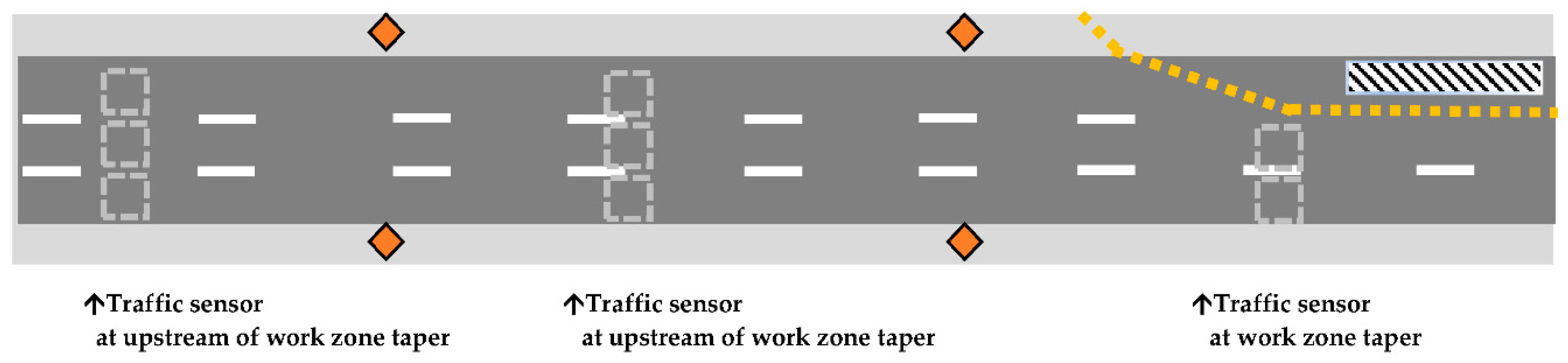
As previously stated, the goal of the calibration is to find the driver behavior parameters that minimize the dissimilarities between traffic stream parameters that are obtained from the simulation model and ground truth traffic stream parameters. Traffic stream parameters include speed and flow at the work zone taper, and speed and flow at locations upstream of the work zone taper. Ground truth traffic stream parameters are often collected by traffic sensors, as shown in Figure 1. Traffic stream parameters in the simulation models are often collected by coding data collection points in the simulation model.

Equation (2) describes the objective function in detail. Average absolute relative error (AARE) is selected as the measure of dissimilarity between the simulation data and ground truth data. The first expression of Equation (2) represents the AARE between the flow rate obtained from the simulation model and the ground truth flow rate at the taper. The second statement of Equation (2) calculates the AARE between the speed obtained from the simulation model and the ground truth speed at the taper. The third expression computes AARE between the simulation and ground truth flow rate at locations upstream of the taper. The fourth expression calculates AARE between the simulation and ground truth speed at locations upstream of the taper.

$$f\left(\mathit{x}\right)={{\displaystyle \sum }}_{d=1}^k{{\displaystyle \sum }}_{i=1}^n\alpha \times \left|\frac{{\widehat{q}}_{i,d}-q_{i,d}}{q_{i,d}}\right|+{{\displaystyle \sum }}_{d=1}^k{\displaystyle \sum }_{i=1}^n\beta \times \left|\frac{{\widehat{u}}_{i,d}-u_{i,d}}{u_{i,d}}\right|+\cdots$$

$${{\displaystyle \sum }}_{d=1}^k{\displaystyle \sum }_{j=1}^m{\displaystyle \sum }_{i=1}^n\gamma \times \left|\frac{{\widehat{v}}_{i,j,d}-v_{i,j,d}}{v_{i,j,d}}\right| + {{\displaystyle \sum }}_{d=1}^k{\displaystyle \sum }_{j=1}^m{\displaystyle \sum }_{i=1}^n\delta \times \left|\frac{{\widehat{s}}_{i,j,d}-s_{i,j,d}}{s_{i,j,d}}\right|$$

(2)

where,

• ${\widehat{q}}_{i,d}$ and ${\widehat{u}}_{i,d}$ are flow rate and speed at the taper at time interval $i$ on day $d$ obtained from the simulation model.
• $q_{i,d}$ and $u_{i,d}$ are ground truth flow rate and speed at the taper at time interval $i$ on day $d$.
• $k$ is the total number of days that work zone was simulated.
• $n$ is the total number of simulation time intervals in each day.
• $m$ is the number of data collection points upstream of the work zone.
• $\alpha$ and $\beta$ are weights of average absolute relative error of flow and speed at the taper.
• ${\widehat{v}}_{i,j,d}$ and ${\widehat{s}}_{i,j,d}$ are flow and speed at location j at time interval i on day $d$ obtained from the simulation model.
• $v_{i,j,d}$ and $s_{i,j,d}$ are ground truth flow and speed at location j at time interval i on day $d$.
• $\gamma$ and $\delta$ are weights of average absolute error of flow and speed at data collection points upstream of the work zone.

Table 2. Solution bounds for driver behavior parameters.

	Parameter	Lower Bound	Upper Bound
1	$CC{1}_P$	0.9 s	2.0 s
2	$CC{1}_T$	1.5 s	3.5 s
3	$CC{2}_P$	3.99 m	12.00 m
4	$CC{2}_T$	4.57 m	17.76 m
5	$LC$	200 m	1200 m

provides the solution bounds for the driver behavior parameters. The range of passenger car parameters was selected to cover all the values that were suggested by other researchers. The upper bound of the heavy-vehicle driver behavior parameters was calculated to be 50% higher than the passenger car upper bounds. Enumerating all the possible solutions for the driver behavior model parameter will result in approximately 1 billion solutions. Since the brute-force approach to finding the optimal solution is not practical, the Particle swarm optimization (PSO) algorithm was proposed to find the optimum driver behavior parameters for passenger cars and heavy vehicles. PSO is a population based stochastic optimization algorithm. This algorithm is inspired by the social behavior of bird flocks where a group of individuals named particles travel through the search region at steps. At the end of each step, all particles are evaluated according to the objective function and a new velocity for each particle is selected. The velocity of each particle is determined based on the position of best particle in the swarm and based on the best position of each particle in the previous steps. The optimization steps are repeated until there is no significant improvement in the objective function value or until the maximum number of iterations is achieved [28].

The PSO algorithm starts with creating an initial swarm of size N, shown as $\left\{{\mathit{x}}_1^0,\dots ,{\mathit{x}}_i^0,\dots ,{\mathit{x}}_N^0\right\}$ where ${\mathit{x}}_i^0$ is the initial position of particle $i$, ${\mathit{x}}_i^0=\left\{CC{1}_{P,i}^0,CC{2}_{P,i}^0,CC{1}_{T,i}^0,CC{2}_{T,i}^0,L{C}_i^0\right\}$. The superscript $0$ indicates that the ${\mathit{x}}_i^0$ is the initial position of the $i^{th}$ particle. In other words, the current iteration $k$ of the algorithm is zero. The initial position of a particle is randomly selected within the bounds of each parameter. A set of initial velocities, $\left\{{\mathit{v}}_1^0,\dots ,{\mathit{v}}_i^0,\dots ,{\mathit{v}}_N^0\right\}$, is created for the initial swarm [33,34,35]. Uniform random values within the variable bounds are selected as initial velocity for each particle. In the next step, work zone traffic is simulated based on deriver behavior parameters of a particle and the objective function value of a particle is calculated based on Equation (2). The pseudocode below outlines the remaining steps of the PSO algorithm.

Step 1: For each particle i of the swarm, randomly select a subset of particles in the swarm. Refer to this subset as A

• Step 1.1: Identify $g_i^k$, which is the particle in subset A with the best objective function value,
• Step 1.2: Identity $b_i^k$, which is the best position that particle i has ever achieved
• Step 1.3: Update the velocity of particle $i$ according to Equation (3):

  $${\mathit{v}}_i^{k+1}=\omega {\mathit{v}}_i^k+{\varphi }_1·y_1·\left(g_i^k-x_i^k\right)+{\varphi }_2·y_2·\left(b_i^k-x_i^k\right)$$

  (3)

  where $k$ indicates the current iteration,
  • $\omega$ is the inertia,
  • ${\varphi }_1$ is the social-adjustment weight,
  • $y_1$ and $y_2$ are random uniformly distributed values between 0 and 1,
  • ${\varphi }_2$ is the self-adjustment weight.
• Step 1.4: Update the position of the particle according to Equation (4):

  $${\mathit{x}}_i^{k+1}={\mathit{x}}_i^k+{\mathit{v}}_i^{k+1}$$

  (4)

If the position of ${\mathit{x}}_i^{k+1}$ is at a bound, set the ${\mathit{v}}_i^{k+1}$ to zero.

Step 2: Evaluate all the particles in the ${\left(k+1\right)}^{th}$ iteration of the swarm.

Step 3: If iteration $\left(k\right)$ is less than three, then $\omega =2\times \omega$, otherwise, $\omega =\omega /2$.

Step 4: If the termination condition is not met, return to step 1.

The set of driver behavior parameters (i.e., the particle) that corresponds with the lowest objective function value is selected as the work zone driver behavior parameters. This set of driver behavior parameters is used to simulate the work zone on days that were not used in the calibration process. This is to ensure that the PSO algorithm did not suffer from overfitting and the proposed driver behavior model parameters can be generalized to days that are not previously seen by the model. This process is commonly referred to as “validating” the model, in contrast with “calibration” of the model.

In addition to AARE, Root Mean Square Error (RMSE), Mean Absolute Error (MAE), and the GEH statistic were used to assess the driver behavior parameters. RMSE and MAE were calculated for speed and flow rates that were obtained in 15 min intervals, and GEH was calculated for flow rates that were obtained in one hour intervals. These performance measures are shown in Equations (5) to (7).

$$RMSE=\sqrt{{{\displaystyle \sum }}_{d=1}^k{{\displaystyle \sum }}_{i=1}^n{\left({\widehat{t}}_{i,d}-t_{i,d}\right)}^2/\left(k\times n\right)}$$

(5)

$$MAE={{\displaystyle \sum }}_{d=1}^k{{\displaystyle \sum }}_{i=1}^n\left|{\widehat{t}}_{i,d}-t_{i,d}\right|/\left(k\times n\right)$$

(6)

where,

• ${\widehat{t}}_{i,d}$ is the traffic parameter at time interval $i$ on day $d$ obtained from the simulation model.
• $t_{i,d}$ is the ground truth traffic parameter at time interval $i$ on day $d$.
• $k$ is the total number of days that the work zone was simulated.
• $n$ is the total number of simulation time intervals in each day.

The GEH statistic is another measure that is commonly used to evaluate traffic simulation models [36].

$$GEH={\sum }_{d=1}^k{\sum }_{i=1}^n\sqrt{\frac{2\ast {\left(E_{i,d}-V_{i,d}\right)}^2}{E_{i,d}+V_{i,d}}}$$

(7)

where $GEH$ is the GEH statistic, $E$ is the volume obtained from the simulation model (veh/hr), and $V$ is the ground truth volume (veh/hr). Other variables were defined previously.

4. Case Study

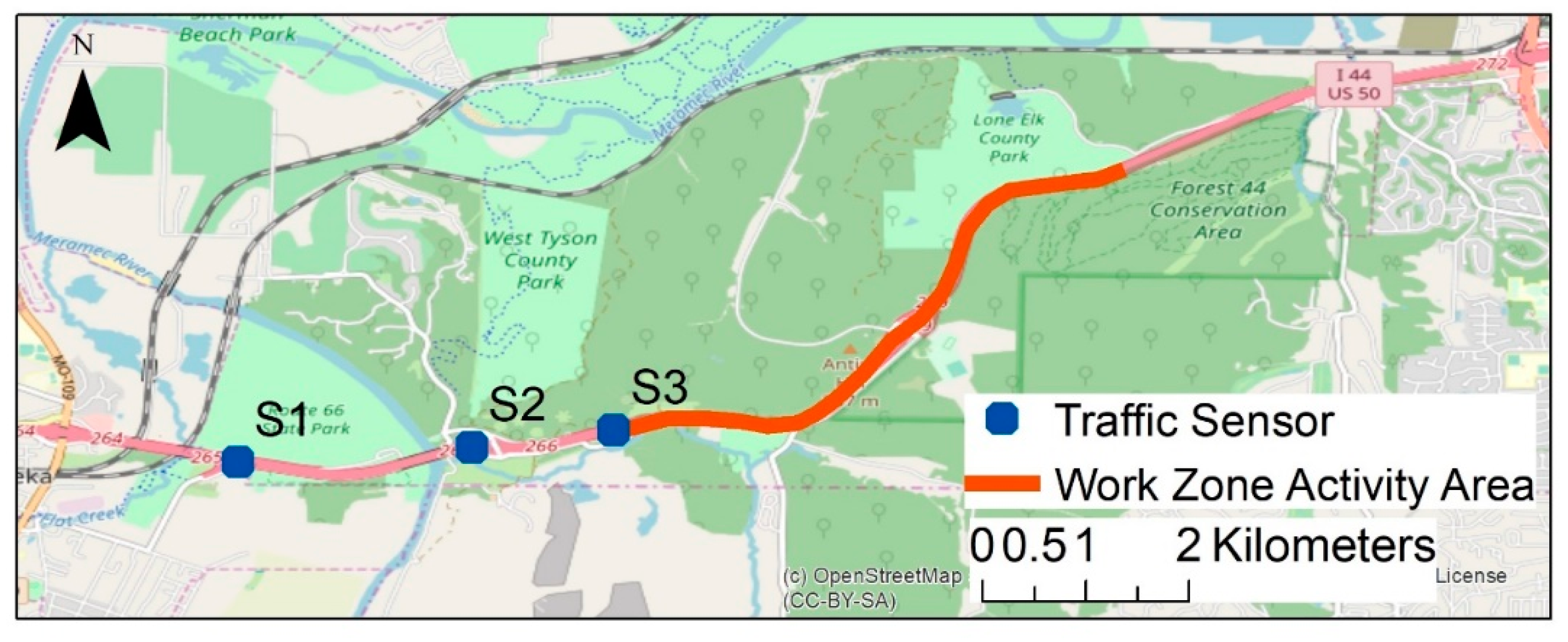
Data from a long-term work zone in the suburbs of St. Louis, Missouri were used to calibrate the driver behavior parameters. The work zone site is located southwest of St. Louis on Interstate 44 (I-44) between Antire Road and Lewis Road. Each direction has three lanes of travel, and one of the three lanes in each direction was closed for a project that involved pavement repairs and road resurfacing. The length of the work area was 5.15 km. The speed limit on Interstate 44 is 105 km/h, and the speed limit was reduced to 88 km/h in the work zone. The freeway annual average daily traffic (AADT) is 68,181, including 8020 heavy vehicles (11.8% of the AADT). No alternative routes were available because of the suburban setting. Portable traffic sensors were installed at the eastbound work zone to collect speed, flow, and occupancy data. Figure 2 shows the location of the work zone and of the portable traffic sensors. Sensor 1 (S1) was placed 2.90 km upstream of the taper, sensor 2 (S2) was installed 1.03 km upstream of the taper, and sensor 3 (S3) was located at the taper. Data that were collected by these sensors were utilized to determine the driver behavior parameters. The sensors’ data were aggregated to 15 min intervals.

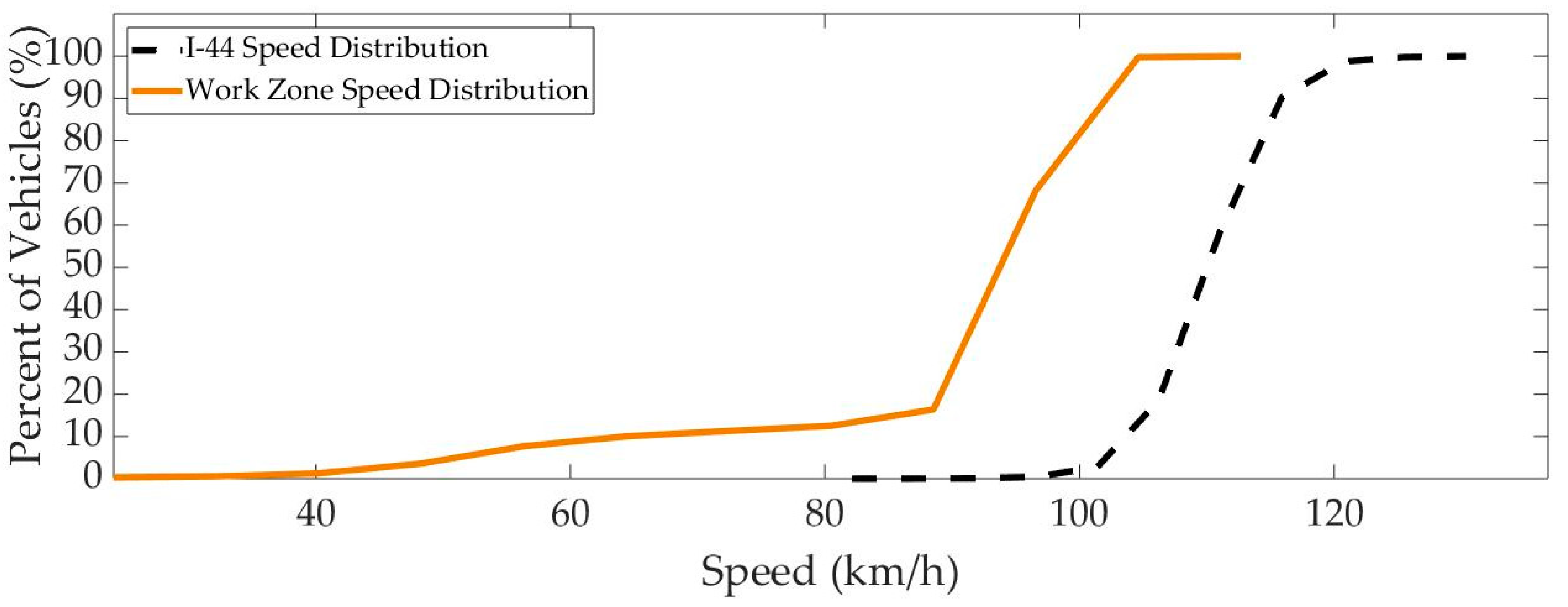
The 4 km segment of I-44, which is upstream of the taper, was coded in VISSIM simulation software. Speed data from S1 and S3 were used to develop desired speed distributions for I-44 upstream of the work zone and for the work area. Figure 3 illustrates these desired speed distributions. The cumulative speed distributions represent freeway speeds when volume was equal to or less than 1400 veh/h/ln at the sensor. In other words, only speed data from free-flow traffic periods were used to develop the cumulative speed distributions (CDFs). This definition is consistent with the definition of free flow speed in Highway Capacity Manual, Sixth Edition. The taper length and location of the work zone speed distribution were determined according to the Manual on Uniform Traffic Control Devices (MUTCD) guidelines for temporary traffic control at work zones [37]. The model was coded to simulate traffic from 4:30 a.m. to 10:00 a.m. Traffic volumes that were measured at sensor S1 were used as vehicle inputs for the model. The simulation period of 4:30 a.m. to 5:00 a.m. was considered a warm-up period; no performance measures were collected during this time. A VISSIM-COM script was written in MATLAB to automatically update the vehicle input volumes for any given day and to run the PSO optimization algorithm.

5. Results and Discussion

The work zone driver behavior parameters were determined through a stepwise implementation of the proposed PSO optimization method that was described in Section 3.

Table 3. The particle swarm optimization (PSO) algorithm search progress.

Step	Number of Particles in the Swarm	Number of PSO Iterations	Number of Days Simulated	Number of Simulation Random Seeds
1	10	43	3	1
2	10	21	3	3
3	10	38	3	5
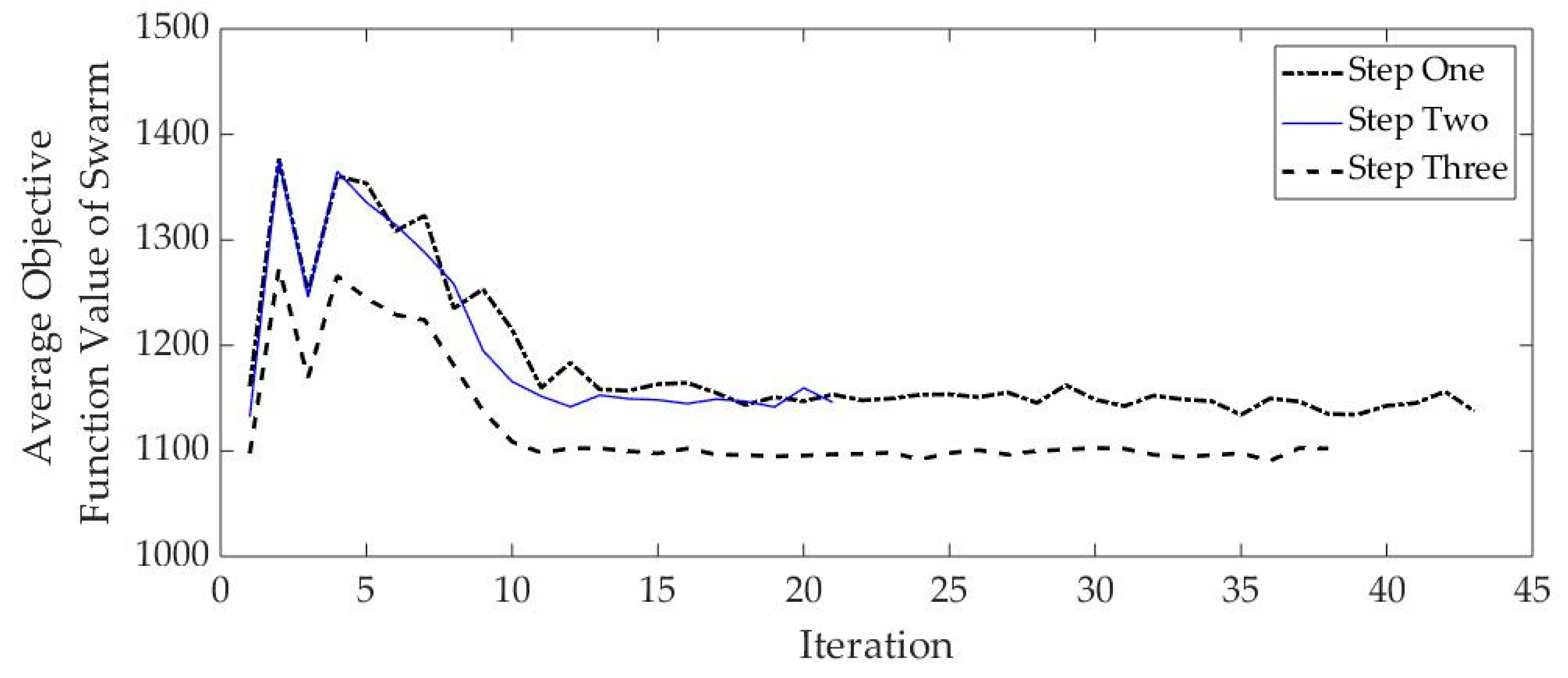
Validation	1	1	10	10

provides calibration parameters for each step and Figure 4 illustrates the PSO objective function value in each step. In the first step, 10 sets of driver behavior parameters were randomly generated and were simulated with three days of data and with one simulation random seed. Ten particles with lowest objective function values were transferred to step 2 to be used as the initial swarm of the optimization process. In step 2, particles were evaluated using three days of work zone traffic data; the simulation of each day was repeated with three different random seeds. Each particle was evaluated by averaging the performance measures that were obtained from each simulation seed. The PSO algorithm stopped at iteration 21 when no significant improvements were observed in the objective function. In step 3, each particle was evaluated using traffic data from three days. Each day was simulated using five different random seeds. The optimization algorithm stopped at iteration 39.

The particle with the smallest objective function value was selected as a possible solution for the optimization problem. The desired time headway was found to be 2.31 seconds for heavy vehicles ($CC{1}_T$) and 1.53 seconds for passenger cars ($CC{1}_P$). The longitudinal following threshold was found to be 17.64 meters for heavy vehicles ($CC{2}_T$) and 11.70 meters for passenger cars ($CC{2}_P$). The lane change distance for both heavy vehicles and passenger cars was assumed to be the same and was found to be 573 meters. These driver behavior parameters were further validated with 10 days of data that were not previously used in the calibration process. Each day was simulated 10 times with 10 different simulation seeds. The overall performance measures for each day were obtained by calculating the average of the performance measures of each simulation. The performance measures for the calibration and validation datasets are listed in

Table 4. Performance measures for the calibration and testing datasets.

Location	Dataset	Flow Rate			Speed
		AARE (%)	RMSE (veh/h/ln)	MAE (veh/h/ln)	AARE (%)	RMSE (km/h)	MAE (km/h)
Upstream	Calibration	5	35	25	23	25	12
	Validation	3	28	17	27	23	13
Taper	Calibration	10	76	58	22	21	18
	Validation	10	78	54	19	20	16

AARE: average absolute relative error; RMSE: Root Mean Square Error; MAE: Mean Absolute Error.

.

Table 4 provides the AARE, RMSE, and MAE for flow rate and speed for the calibration and validation datasets for a location 2.90 km upstream of the work zone taper, and for the taper. The performance measures that were obtained for the calibration and validation datasets are consistent. This consistency indicates that the calibration process did not suffer from overfitting and the proposed work zone driver behavior parameters were able to simulate traffic conditions for previously unseen traffic data. For example, the RMSE for flow rate at the taper for the calibration dataset was 75 veh/h/ln, while the RMSE for flow rate at the taper for the validation dataset was 78 veh/h/ln. Similar trends were observed at a location upstream of the taper and for speed. The GEH statistic was calculated for the calibration and validation datasets. The GEH statistic for the calibration dataset was 1.17 and the GEH statistic for the validation dataset was 1.48. The GEH statistic for both the calibration and testing dataset were less than 5, indicating that vehicles were able to enter the simulation network. While the performance measures for flow rate are ideal for both calibration and validation datasets, the AARE of speed for the calibration and validation datasets ranged between 19% and 23%, and the MAE of speed for the calibration and validation datasets ranged between 12 km/h to 18 km/h. These error indexes are attributed to the work zone desired speed distributions, as discussed below.

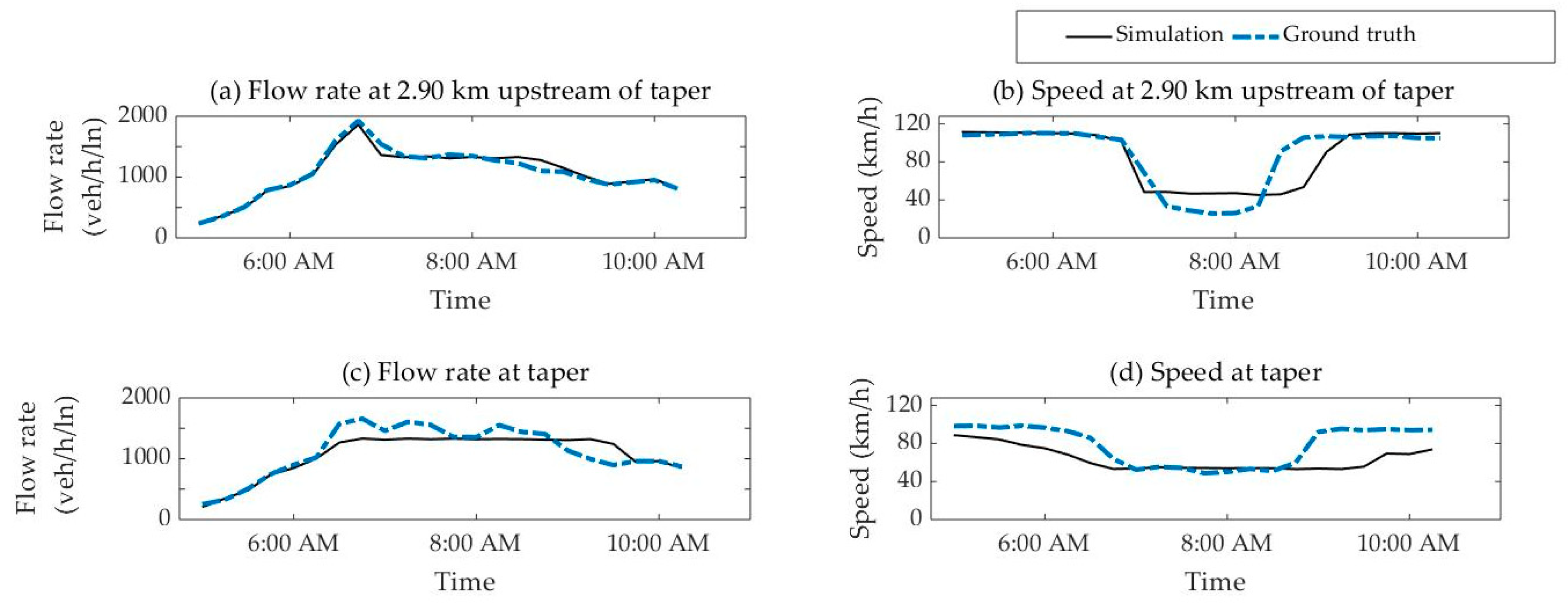
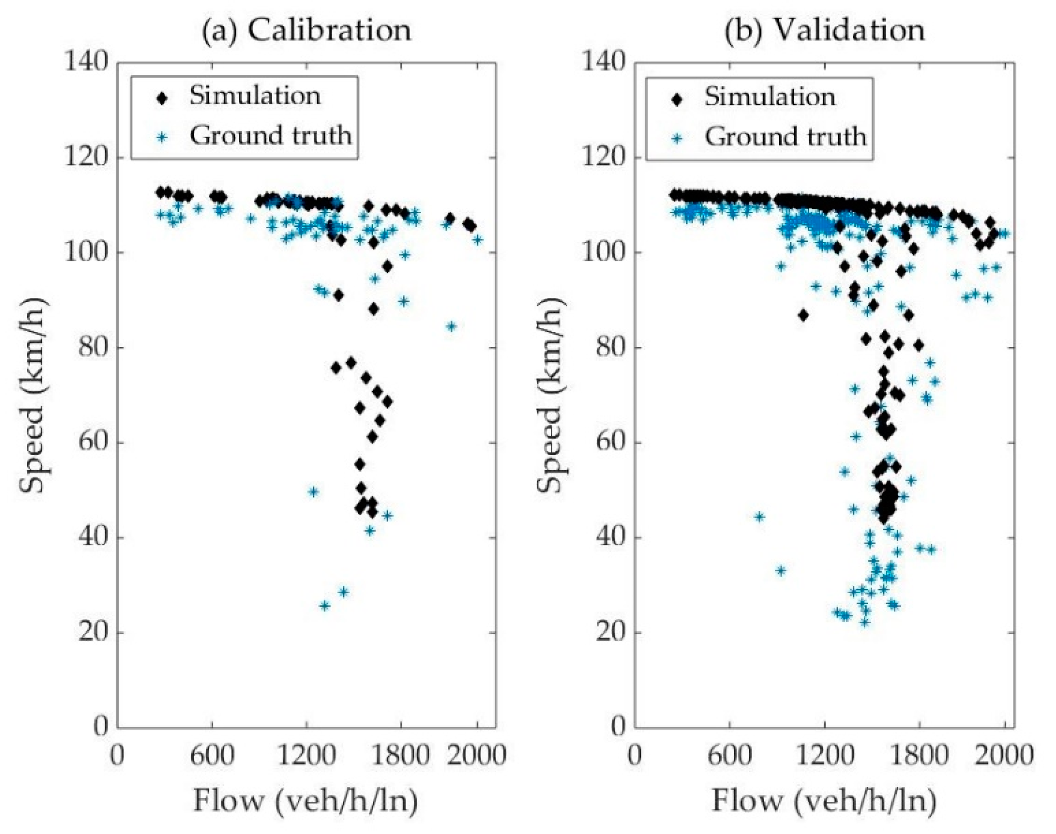
Figure 5 illustrates the time series of simulation and ground truth flow rate and speed data that were obtained for a day in the validation dataset. Figure 6 shows the speed-flow data for the calibration dataset and validation dataset at the taper. The simulation model replicates the flow rates that were observed in the field fairly consistently; however, it overestimates the speed upstream of the work zone and underestimates the speed at the taper. The overestimation and underestimation of speed is potentially attributed to the desired speed distributions that were defined for upstream of the work zone and for the taper as the simulation software is obligated to replicate the speed CDFs that are shown in Figure 3. These speed distributions were defined based on the HCM definition and force the vehicles to drive within this range. In future research, guidelines can be developed for defining desired speed distributions at work zones. Calibration and validation speed-flow plots illustrated in Figure 6 indicate that driver behavior models produced the work zone capacity that is observed in the field.

Previous studies often focused on replicating capacity at the work zone taper and did not report error indexes for flow and speed at locations upstream of the work zone [11,14,18]. The error indexes that were obtained for work zone driver behavior parameters are consistent with error indexes that were reported for traffic simulation models at other types of transportation facilities. Dong et al., [10] reported a GEH statistic of 3.84 for the calibration of driver behavior parameters on Iowa freeways. Giuffrè et al., [13] reported a GEH statistic of 5 for traffic simulation models that were developed for roundabouts. The GEH statistic that was obtained for work zone driver behavior parameters was 1.17 and 1.48 for the training and validation datasets, respectively. GEH statistic values lower than 5 are acceptable, with smaller values being more desirable. Chen et al., [23] reported MAE values for speed ranging from 15 km/h to 20 km/h for the calibration of driver behavior parameters for various weather conditions. These speed MAE values that were reported for work zone driver behavior parameters are between 12 km/h and 18 km/h, which is comparable to MAEs reported in [23].

There are trade-offs between the training dataset size and the validation dataset size; increasing the training dataset size might improve the performance measures obtained from the simulation model, however a larger training dataset will increase the computational cost of the optimization process. The performance measures that were obtained for the training and validation datasets are consistent with performance measures reported in the literature [10,13,23]. This indicates that three days of training data was sufficient for deriving driver behavior parameters from field data. For future research, it is recommended to develop work zone driver behavior parameters for various traffic compositions, for various lane closure configurations, and for short-term and long-term work zones. Another opportunity for future research is to develop computationally efficient methods to calibrate all the 10 parameters of the Wiedemann 99 model for passenger cars and heavy vehicles in work zones.

6. Conclusions

Traffic simulation models allow transportation agencies to conduct detailed analyses of work zone mobility performance measures. Traffic simulation is a particularly advantageous tool when a work zone temporary traffic control plan includes complex lane split and lane shift patterns or when there are concerns about the impact of the work zone on upstream transportation facilities.

A key step in coding the traffic simulation model is calibration of the model parameters that relate to driver behavior. A common goal in this process is to ensure that the simulation model replicates the work zone capacity values that are observed in the field. In this paper, work zone driver behavior model parameters were calibrated such that both flow and speed values were replicated at the taper and at roadway segments upstream of the work zone. The paper further investigated the hypothesis that heavy vehicle and passenger car driver behavior model parameters are different in work zones. Calibration of driver behavior parameters at a long-term 3-to-2 work zone on Interstate 44 in St. Louis, Missouri indicated that the desired time headway for heavy vehicles is 2.31 seconds, while the desired time headway for passenger cars is 1.53 seconds. The longitudinal following threshold was found to be 17.64 m for heavy vehicles and 11.70 m for passenger cars. The lane change distance for both heavy vehicles and passenger cars was assumed to be the same and was found to be 573 m. The simulation software does not allow users to set different lane change distances for heavy vehicles and passenger cars. It is recommended to study the impact of different lane change distances for heavy vehicles and passenger cars in future research.

The calibration of a simulation model is an optimization problem where the objective is to find a set of driver behavior parameters that replicates traffic conditions that are observed in the field, and the solution region is a multidimensional space of feasible values for driver behavior parameters. This paper proposed a framework based on the particle swarm optimization (PSO) algorithm to calibrate the driver behavior model in the work zone. The PSO framework is computationally efficient compared to the brute-force search methods that were used in the literature and was successful in identifying optimal driver behavior parameters.