Residential Land Use Change in the Wissahickon Creek Watershed: Profitability and Sustainability?

Abstract

The Wissahickon Creek Watershed is one of five major watersheds in the Philadelphia metro region. The main objective of the work in this paper was to determine and compare the energy and environmental impacts of placing housing in the Watershed according to profitability and environmental sustainability criteria, respectively, in the context of increasing urbanization. Future population and employment for the Watershed have been projected by the Delaware Valley Regional Planning Commission. Housing requirements for the projected populations in each municipality were computed, and their location was influenced by the local zoning ordinances. Suitability analysis using ArcGIS 10.6 generated areas for development based alternatively on profitability and local sustainability. CommunityViz 5.2 Scenario 360 software was used to place buildings within the appropriately-zoned areas. Using Argonne National Laboratory’s Greenhouse Gases, Regulated Emissions, and Energy Use in Transportation (GREET1 2018) software and water quality monitoring information from the Philadelphia Water Department, impacts were directly estimated. The impacts were related to effects on ecosystem functioning, ecosystem goods and services, and broad value estimated for the latter. The effects were used to indicate what might be appropriate policies to reduce the negative environmental consequences of residential development in the watershed. Unexpectedly, the environmental impacts of the profitable and sustainable scenarios were not very different. This suggests that profitability and sustainability need not be mutually exclusive.

1. Introduction

In 2018, it was estimated by the Population Division of the Department of Economic and Social Affairs of the United Nations that 55% of the world’s inhabitants live in urban areas. This is projected to rise to 68% by 2050 [1]. The movement to “major urban agglomerations” involves a choice between the cities and their suburbs and ultimate land use change. To accommodate this increasing population, residential development can take place on infilled or reclaimed land with higher density and existing infrastructure, or on newly-developed land with lower density and little or no infrastructure.

The work for this paper involved a major metropolitan watershed that encompasses both a segment of the City of Philadelphia, and all or part of 15 suburban municipalities. The main objective was to determine and compare the economic, energy, and environmental impacts of scenarios of placing housing according to profitability criteria on the one hand, and environmental sustainability criteria on the other. The profitability criteria involved the profit generated by the average housing unit sale, as well as neighborhood characteristics (e.g., an income index and a crime index), in each zip code within the municipalities. The sustainability criteria included proximity to infrastructure and institutions already in place. Both scenarios had areas that were restricted from development. The prior expectations were that the scenario based on profitability would have higher profit, and that based on sustainability would have significantly smaller environmental impacts.

Different aspects of the work in this paper have been investigated by previous authors. Much of the literature on the geographical aspects of housing, as shown in Hasanzadeh et al. [2], deals with the demand side. Using public participation Geographic Information Systems (GIS), the authors investigated whether people inhabited the parts of the urban structure that their classification of urbanists, semi-urbanists, and nature-lovers suggested they would. The majority did not. On the housing supply side, Saiz [3] used US Geological Survey Digital Elevation Model and National Land Cover data in GIS to examine geographical restrictions on supply in US metropolitan statistical areas over 500,000. The author concluded that those areas with greater restrictions (including regulatory) had higher housing prices and a lower price elasticity of housing supply. Hudson [4] contrasted the treatment of sustainable housing development with the traditional approach in the US, of development without much concern for natural capital. Sandberg [5] approached sustainable housing by looking at proposed downsizing of dwellings in Finland. Musse et al. [6] applied a “backcasting” approach to providing low-income housing in a Brazilian city through a vision of a sustainable future. Koshkar et al. [7] studied the impact of urban growth and residential densification on urban–suburban green space and ecosystem services in sections of the Stockholm region. Göçmen, Z. et al. [8] surveyed many county and municipal governments in Wisconsin, USA to ascertain the types of sustainable practices, e.g., New Urbanism, that the agencies implemented with respect to future residential development. Stachuro [9] examined the behavioral implications of creating “eco-districts” with their own sustainable infrastructure within urban areas. Hanlon [10] concentrated on suburban re-development after decades of expansion in Baltimore, MD, USA. Sorrentino et al. [11] and Sorrentino et al. [12] used housing buildout in an urban–suburban watershed to determine the relative impacts of alternative development scenarios. Dunphy et al. [13] proposed a business model that values sustainable retrofit at more than monetary values and involved co-production by sellers and buyers.

Use of the GREET 2018 model to estimate air pollution and greenhouse gas emissions appeared in Almeida et al. [14]. Using life-cycle analysis, the focus was on how different battery technologies would influence electric automobile emissions over time. Their approach was similar to the work in this paper in that scenarios were evaluated in terms of emissions. However, their scale was national and not related per se to housing location.

In the water-related dimension, a recent example of the hydrological modeling approach is Guo et al. [15]. The authors incorporated low impact development (LID) into a Storm Water Management Model (SWMM), and built scenarios showing the effects of green roofs, permeable pavement, and other LID technologies on runoff. Chao et al. [16] reported the results of implementing sustainable residential development on water consumption in two urban regions in Australia. Xian et al. [17] used remote sensing to assess the impacts on water-quality parameters of increased impervious surface and population density in the Tampa Bay, FL, USA watershed. Nesheim and Barkved [18] evaluated the sustainability potential of watersheds altered for hydropower production in Norway, using a process that combined ecosystem services valuation with the value of uses that accrue to beneficiaries from the human intervention itself.

Watershed planning can take the form of the very sophisticated decision-making paradigms in Azarnivand and Banihabib [19], where complex and heterogeneous inputs were reconciled with stakeholder concerns to achieve sustainable watershed development. In a less technical and more practical approach, Berg and BenDor [20] proposed the use of form-based regulation to replace traditional zoning in land-use decisions, to accomplish the dual goals of a superior built environment and water quality protection in eastern North Carolina, USA. Using a planning and design-centric approach at a metropolitan scale, Ahmed et al. [21] analyzed urban spatial morphology, street connectivity, and water drainage patterns to develop a regional Blue-Green Infrastructure network, which identifies suitable locations for future development in order to accommodate highly-increasing urban populations in a sustainable way. Fan and Shibata [22] used the Soil and Water Assessment Tool (SWAT) to estimate amounts of the hydrological provisioning services of irrigation, electricity production, and household usage. The authors combined the SWAT outcomes with a cost assessment of each hydrological ecosystem service (e.g., water usage by hydropower plants and households, and for irrigation in crop production) in the watershed. Areal zonation was used to analyze the spatial conservation prioritization of the ecosystem services. A common thread in the recent literature is that sustainable development is becoming increasingly imperative as urban–suburban areas grow.

The next section contains a description of the study area and the various elements of the methodology used to generate the results. These results are shown in the third section. A discussion of the results takes place in the fourth section, followed by policy implications, some conclusions, and future research goals.

2. Methodology

Once the geographical area was chosen, data were collected from the sources listed in Table 2. Two suitability analyses were performed using ArcGIS 10.6 that generated the areas meeting the criteria for each scenario. A buildout using CommunityViz 5.2 Scenario 360 placed the maximum number of housing units in the WCW, and those within the suitable areas were counted. The housing units were overlaid on the zip codes, census tracts, and sub-basins to estimate the various impacts. The impacts were related to ecosystem goods and services valuation.

2.1. The Geographical Study Area

The Wissahickon Creek is located in southeastern Pennsylvania (PA) and flows from its headwaters approximately 37 kilometers south, where it then drains into the Schuylkill River in Philadelphia (Figure 1). The Philadelphia metro region is the seventh largest in the US. The Wissahickon Creek Watershed (WCW) is one of five major creek watersheds in that region. The preservation of its natural capital allows it to provide several ecosystem goods and services to a variety of beneficiaries.

The WCW covers an area of 166 km². Its topography is characterized by both flat and sloping terrain. There are steep slope areas near Sandy Run and along the main stem of the Wissahickon Creek. The elevation of the watershed ranges from approximately 7 meters (m) in the south to 149 m in the north. Much of the upper portion of the watershed lies within the Gettysburg–Newark Lowland Physiographic Province. The lower portion is within the Piedmont Lowlands and Piedmont Uplands Provinces. The bedrock geology of the watershed is diverse, with more than 10 different geologic formations underlying the area. Two of the larger bedrock formations are the Stockton and the Lockatong.

The climate of the region is characterized by warm summers, cold winters, and moderate springs and autumns. The mean annual temperature is roughly 12 degrees Celsius. The approximate average annual precipitation is 107 centimeters (cm) and snowfall is 49 cm.

From the early 17th Century, the WCW was inhabited by the Lenni-Lenape Indians, who subsisted on the abundant hunting, fishing, and farming opportunities there [23]. The land uses of the WCW remained forest and agricultural for centuries, until it became developed as part of the inner-ring suburbs of Philadelphia in the mid-to-late 1800s. By the turn of the 20th century, many of the communities had direct rail connections with Philadelphia. Following World War II and throughout the 1950s, a surge in residential and commercial development occurred, spurred by the opening of manufacturing plants and shopping centers, and the construction of major roadways.

Today, the watershed contains all or portions of 15 municipalities in Montgomery County and stretches into the City of Philadelphia. The 2010 population for the watershed was approximately 160,000 [24]. It contains a mix of land uses, including agriculture, commercial, residential, institutional, and greenspace. (Figure 2). However, development that has occurred did not always take place in a well-planned manner, and there is what some consider to be sprawl in many areas. In PA, planning and growth management are the responsibility of the more than 2500 municipalities which exercise zoning, development, and land use controls under the authority of the PA Municipalities Planning Code Act of 1968. Counties prepare comprehensive plans to guide land use and growth management of each municipality, but the latter are not required to follow them [25]. Municipalities often make decisions without regard for their neighbors, thereby thwarting plans to manage development regionally to contain sprawl. Competition among municipalities for taxable properties exacerbates sprawl [26]. While conservation groups and government agencies have been successful in preserving many acres of open space in the WCW, large portions of the remaining open space are in private ownership and could face future development [27].

The PA Department of Environmental Protection (PA DEP) has classified the Wissahickon and its tributaries as a trout-stocked fishery. The most popular fish caught are rainbow trout, smallmouth bass, and brown trout. Other species in the Creek include largemouth bass and sunfish.

The Wissahickon Creek Conservation Landscape contains 1933 acres of forest within its 6517 acres. Redback and two-sided salamanders, American toad, bullfrog and green frog, eastern painted turtle, and northern ringneck and black-racer snakes, are among the native inhabitants of the landscape. The Green Ribbon Preserve follows the Creek, and much of it is floodplain. Tree species in the most eroded areas along the Creek include sycamore, box-elder, slippery elm, and red and silver maple. The understory is sparse due to frequent scouring by floodwaters and high deer presence. Swamp white oak, pin oak, white ash, green ash, black walnut, cottonwood, shagbark and shellbark hickory, red maple, honey locust, and tulip trees make up the floodplain-terrace communities, while shrubs and vines include spicebush, silky dogwood, northern arrow-wood, and summer and frost grape. On the herbaceous layer, one can find enchanter’s nightshade, white avens, skunk cabbage, fowl mannagrass, New York and sensitive fern, jewelweed, rice cutgrass, jumpseed, and false nettle. Riparian Highlands display red oak, American beech, tulip tree, mockernut hickory, white ash, white oak, and flowering dogwood. Spicebush, blackhaw, and northern arrow-wood dominate the shrub layer. Herbaceous species include mayapple and spring-beauty. Besides the usual forest fauna of squirrels, chipmunks, and other creatures, two hundred different species of birds over the course of a year are attracted by the mixed-habitat of waterway, woodland, and meadow, as well as the richly-landscaped private properties which surround the park [27].

Like many other areas in the modern PA landscape, however, the Wissahickon Valley is rife with invasive species. Among plants, this is particularly true in the herbaceous and shrub layers. Obtuse-leaved privet, Japanese honeysuckle, false indigo, siebold viburnum, Indian strawberry, stinging nettle, and Japanese knotweed are common invasives [27]. In the context of a generally declining bird population, a specific problem in the Wissahickon is the negative impact that feral pet cats have on the songbirds and other year-round animal residents [28].

The headwaters of the Creek begin in a stormwater basin for a parking lot of the Montgomery Mall in Montgomery Township, Montgomery County. The impact of human development on the Creek is evident from its origin. Development and human activities have threatened water quality and quantity. Some threats include the discharge of sewage treatment plant effluent, deforestation of riparian areas, and increased sedimentation. The base flow of the Creek is low and has been reported to be dry at times in the headwaters. Causes of low base flow can be attributed to groundwater pumping and increased impervious surface, which decreases infiltration. In fact, over 30 percent of the watershed is covered by impervious surface [29]. In addition, some of the groundwater withdrawals in the upper portion of the watershed are exported to municipalities outside of the area as public water supply.

Because of the low base flow, many portions of the Creek experience flows almost entirely derived from treated effluent discharged by the five publicly-owned wastewater treatment facilities during dry weather conditions. According to the Philadelphia Water Department (PWD) [30], sewage treatment facilities comprise 99% of the total point source discharges in the watershed. There have been instances of industrial toxin releases and bacteria releases from failed sewage treatment plant processes, causing the PA DEP to issue temporary bans on fishing, drinking, and swimming [31].

The Wissahickon Creek and many of its tributaries are considered impaired waters by the Pennsylvania Integrated Water Quality Monitoring and Assessment Report [32]. In 2003, the US Environmental Protection Agency (EPA) Region III established Total Maximum Daily Loads (TMDLs) for nutrients and siltation in the WCW [33]. As noted above, the major source of nutrients in the Creek is the wastewater treatment plants. These nutrients can cause eutrophic conditions, in which bacterial decomposition of excess algae depletes oxygen. In addition, sediment from erosion of its banks due to stormwater runoff can add nutrients.

In order to address stormwater runoff, water quality, and flooding problems in the WCW, an Act 167 Stormwater Management Plan has been completed [34]. Act 167 Plans are required under the Pennsylvania Stormwater Management Act of 1978, which directs each county in PA to prepare and adopt a plan for each designated watershed. The WCW’s Act 167 plan provides an assessment of stormwater conditions and has produced a model stormwater ordinance for adoption by municipalities to implement best stormwater management practices.

Since the municipalities in the WCW are anticipated to continue growing in population and employment at a steady pace over the next several decades [35,36], it is important to balance the current and future needs of land and water.

2.2. Building Two Residential Development Scenarios

Lyle [37] discusses the use of “semi-formal” models in ecological planning. By semi-formal, the author means models that avoid strict quantification of all involved processes, but convey order, form and function through simplicity and visual communication. The scenario analysis performed in this work falls in that category. While mathematically specifying the complex ecological functioning of the WCW described in the previous section was avoided, land use and other publicly-available information was used to create a context for the analysis. Suitability models in ArcGIS 10.6 [38] designated non-restricted areas within the WCW that were suitable with respect to profitability and sustainability respectively. A housing distribution/buildout model in CommunityViz Scenario 360 [39] placed housing units within the zoning restrictions of the municipalities in the WCW.

The Delaware Valley Regional Planning Commission (DVRPC) [35], the federally-designated Metropolitan Planning Organization for the region, has published projected population changes for each municipality in its domain to 2045. In what follows, only 2045 estimates were used to place housing, although projections are given for five-year intervals up to that year. Average occupancy is known for each municipality in the WCW, and these were divided into the added population estimates to get the estimates of new housing units. Average occupancy is assumed to remain constant over the entire period. Using the 2015 updates to the 2010 Census and 2015–2016 data on occupancy,

Table 1. Population projections and housing units needed.

Municipality	2015 Pop	2015–2016 Occupied Units	2015* Pop/ 2016 Units	2045 Pop	2015 to 2045 Pop -Change	Housing Units Needed	% Muni in the WCW	Housing Units Needed in the WCW
Abington Township	55,590	20,955	2.65	59,083	3493	1317	0.2294	302
Ambler Borough	6505	2644	2.46	7422	917	373	1	373
Cheltenham Township	37,014	14,349	2.58	39,607	2593	1005	0.0139	14
Horsham Township	26,587	9964	2.67	32,541	5954	2231	0.056	125
Lansdale Borough	16,512	6467	2.55	19,152	2640	1034	0.2365	245
Lower Gwynedd Township	11,548	4567	2.53	12651	1103	436	0.8829	385
Montgomery Township	26,025	9255	2.81	28735	2710	964	0.1401	135
North Wales Borough	3250	1342	2.42	3392	142	59	1	59
Springfield Township	19,574	7419	2.64	20,574	1000	379	0.0734	28
Upper Dublin Township	26,211	9441	2.78	29,745	3534	1273	0.9457	1204
Upper Gwynedd Township	15,928	6340	2.51	17,053	1125	448	0.903	405
Upper Moreland Township	24,231	9537	2.54	25,749	1518	597	0.6186	369
Whitemarsh Township	17,663	6710	2.63	20,476	2813	1069	0.029	31
Whitpain Township	19,180	7153	2.68	20,661	1481	552	0.5638	311
Worcester Township	10,435	3720	2.81	12,943	2508	894	0.4168	373
Philadelphia City/County	1,567,443	582,594	2.69	1,696,133	128,690	47,832	0.064	3061

was compiled.

As noted, what differentiates the two scenarios below is the focus on profit in the one and on sustainability in the other. These manifested themselves in the criteria used for each suitability analysis. While profit is widely known as revenue minus cost, the concept of sustainability is not so precise. The scenarios will be labeled ECON and ENV, the latter based on the notion of metropolitan sustainability [40]. This author argued for sustainability that included, among other things, compact urban design, conservation of open space and sensitive ecosystems, decreased automobile use, appropriately-placed housing, and reduced waste and pollution.

Table 2. The sources of data for suitability and buildout.

Data	Source	Year of Publication
Land Use	DVRPC	2015
Floodplains: 100, 500 years	CSC	2016
Streams	CSC	2016
Slope	CSC	2016
Parks and Open Spaces	DVRPC	2015
Points of Interests (School, Place of Worship, Hospital/Clinic, Employment Center, College/University)	CSC	2016
Wetlands	CSC, DVRPC	2016
Bus Stops	DVRPC	2015
Train Stations	S.E. Penn. Transportation Authority	2014
Zip Codes	PA Spatial Data Access/US Census	2016
House Construction Cost	Means Residential Construction Cost Data	2018
Housing Prices	Trulia.com	2018
Average Income Tax Rate	US Internal Revenue Service	2018
Mortgage Rate	Wall Street Journal	2018
Zoning ordinances of the 15 municipalities in the WCW	Municipal Web Sites	2019

gives the sources of data for the suitability analyses and the residential buildouts. DVRPC was referred to above. CSC is the Center for Sustainable Communities at Temple University, SEPTA is the Southeastern PA Transportation Authority, and PASDA is the PA Spatial Data Access.

2.2.1. The Economically Suitable Scenario: ECON

In general, housing demand is largely a function of the price of the house, the income of the buyer, and other “hedonic” characteristics of the relevant neighborhood. Examples of the latter are the quality of the school system and the safety of the neighborhood. The characteristics of the individual house, such as style, number of bedrooms and bathrooms, are also determinants of demand. However, since the object of the present study was location, the individual characteristics of a buyer’s target house were not directly relevant.

The importance of the characteristics of the neighborhood on housing demand is well-established in the literature. For example, Galster et al. [41] showed that the environment, infrastructure, demographics, neighborhood social status, and the community institutions all have an influence on housing demand. These variables are more difficult to estimate than the particular physical characteristics of the house, but there is a good number of studies that attempted to estimate the hedonic pricing of neighborhood characteristics (e.g., [42,43,44,45,46]). As an example directly relevant to our WCW study, the Reinvestment Fund [46] found in their analysis of the City of Philadelphia that a 1% increase in a structural decline score (based on building vacancies and demolitions, lien sales for unpaid taxes, and water shut-offs due to unpaid bills) in a neighborhood reduced the sales price of homes in that area by $173.84 per m²; a 1% increase in the crime score (based on higher levels of drug use and possession, a range of aggravated and weapons related offenses, and arson) reduced the sales price of homes in that block by $115.82 per m²; and each 1% increase in the school catchment area PA System of School Assessment proficiency score (based on state-wide mathematics and reading tests) increased the sales price of homes in that block by $60.28 per m².

More importantly, since a house is a durable good, the appropriate price that drives demand is not the purchase price, but the after-tax user cost (ATUC) of owning a house (H). Furthermore, in the US, individuals are allowed to deduct the annual interest paid on a house mortgage from their income for tax purposes. The annual mortgage payment is adjusted to reflect the deduction of mortgage interest from federal taxable income. As used by Sorrentino et al. [12], the following equation is the effective price of a house:

$${\mathrm{ATUC}}_{\mathrm{H}}={\mathrm{P}}_{\mathrm{H}}\ast \left(\mathrm{L}\ast \mathrm{MC}+\mathrm{M}+\mathrm{RET}\right)+\mathrm{U}-{\mathrm{P}}_{\mathrm{H}}\ast \mathrm{L}\ast \mathrm{MR}+\mathrm{RET})\ast \mathrm{ATR}$$

(1)

The variables are designated as follows: P_H is the price of a housing unit; L is the loan-to-value ratio; MC is the mortgage constant; M is the maintenance costs as a percent of P_H; U is the utility costs; MR is the mortgage interest rate; RET is the real estate taxes as a percent of P_H; ATR is the average income tax rate.

Studies of US housing markets agree on the appropriate price of housing as ATUC (e.g., [47,48]). There is also close agreement on the percentages used for maintenance cost, real estate taxes, and average income tax rate. These consensus values were used here. The loan-to-value ratio is the amount of the purchase price that a bank will finance. The mortgage constant is a statistic that, when multiplied by the loan amount, yields the annual payment of principal and interest on a home loan. Utility costs were estimated from actual values for a sample of homes randomly chosen within the WCW zip codes on the Trulia website [49]. Finally, tax savings were deducted from the ATUC due to the deductibility of mortgage interest.

It was assumed here that housing demand drives housing supply [50]. Higher demand in a geographic area (say, due to a highly-ranked school system), causes higher prices in that area. Higher prices make it more profitable for developers to build in that area. Hence, demand-side variables were included in the economic suitability analysis. The focus of this paper was where housing developers locate the new houses they build, subject to the zoning restrictions in the municipalities. Obviously, this is a question of supply and is driven by the developers’ profit motivation. However, the question of whether building sustainably can also be profitable was an important part of this investigation.

Housing supply is modeled by economists as a stock and flow model. The supply is determined by the existing stock minus the removal of deteriorated units plus the addition of newly-built units. However, only the sales of those houses in the existing stock in a specific geographic area determine the market price in that area. The developer decides whether they can make a profit building and selling a house at that price. They simply make the product, sell it in a one-off transaction, and reap the profit as the difference between the sales price and the cost of production. Specifically, developer profit for a single unit is the settlement price minus the salesperson’s commission (generally 6% of the sales price), the settlement costs, land costs (a rule of thumb is that improved lots should be about 25% of the total house cost), housing construction costs, infrastructure costs (water, sewer, roads), “soft” costs (appraisal, permit application, review, and inspection fees), and overhead (generally computed as a standard percentage of the sum of the other costs—usually 10%) [51]. Most previous models of the supply of housing estimate a national or metropolitan region housing supply ([52,53,54]). In this work, a unique approach disaggregated prices and costs by zip codes within the WCW.

Profit data for the zip codes are given in

Table 3. Housing price-related (2018 $) data in the Wissahickon zip codes.

Zip Code	Median House Price ($)	ATUC ($)	Common Level Ratio	Full Price/m2 ($)	House Price/m2 ($)	Build Cost/m2 ($)	Profit/m2 ($)
18936	$232,000.00	$22,383.97	0.6211	1790.05	1342.54	1200.65	141.89
19001	$256,300.00	$22,903.66	0.6211	1872.94	1404.70	1200.65	204.06
19002	$411,250.00	$30,360.64	0.6211	1891.02	1418.26	1200.65	217.62
19006	$353,000.00	$28,420.19	0.6211	1758.84	1319.13	1200.65	118.48
19025	$353,000.00	$28,791.55	0.6211	1750.55	1312.91	1200.65	112.27
19031	$300,500.00	$24,484.02	0.6211	1922.99	1442.24	1200.65	241.60
19034	$475,000.00	$34,937.43	0.6211	2020.19	1515.14	1200.65	314.50
19038	$230,000.00	$22,190.97	0.6211	1881.87	1411.40	1200.65	210.76
19044	$214,500.00	$18,944.40	0.6211	1740.54	1305.40	1200.65	104.76
19075	$242,750.00	$22,560.24	0.6211	1834.72	1376.04	1200.65	175.40
19090	$200,850.00	$19,779.38	0.6211	1609.00	1206.75	1200.65	6.11
19118	$452,000.00	$32,034.64	0.3058	2271.53	1703.65	1200.65	503.00
19119	$233,200.00	$19,066.74	0.3058	1311.92	983.94	1200.65	–216.71
19127	$180,000.00	$14,214.45	0.3058	1456.91	1092.68	1200.65	–107.97
19128	$207,500.00	$18,126.17	0.3058	1578.33	1183.74	1200.65	–16.90
19129	$153,000.00	$14,706.29	0.3058	1561.64	1171.23	1200.65	–29.41
19144	$127,000.00	$12,907.87	0.3058	728.51	546.38	1200.65	–654.26
19150	$128,000.00	$13,519.67	0.3058	1025.81	769.36	1200.65	–431.29
19422	$439,000.00	$30,817.25	0.3058	1819.65	1364.74	1200.65	164.10
19428	$338,000.00	$25,912.26	0.6211	1823.21	1367.40	1200.65	166.76
19436	$439,900.00	$30,249.14	0.6211	1841.18	1380.89	1200.65	180.24
19444	$373,750.00	$27,693.02	0.6211	1936.01	1452.01	1200.65	251.36
19446	$243,500.00	$21,592.01	0.6211	1622.13	1216.60	1200.65	15.96
19454	$260,000.00	$21,370.06	0.6211	1827.19	1370.39	1200.65	169.75
19462	$335,000.00	$26,221.99	0.6211	1904.15	1428.11	1200.65	227.47

.

Table 4. Neighborhood characteristics data in the WCW zip codes.

Zip Code	Educational Attainment	Index of Household Income	Crime Index	School District Name	School District Rating
18936	13	1.81	1	North Penn	0.748
19001	14.08	0.8	3	Abington	0.826
19002	15.72	0.89	3	Wissahickon	0.931
19006	15.81	0.85	3	Lower Moreland	0.907
19025	17	1.33	1	Upper Dublin	0.924
19031	15.41	0.92	3	Colonial	0.881
19034	16.1	1	6	Upper Dublin	0.924
19038	15.05	0.83	6	Cheltenham Township	0.582
19044	11.14	0.81	6	Hatboro-Horsham	0.665
19075	14.81	0.88	1	Springfield Township	0.787
19090	11.32	0.75	6	Upper Moreland	0.726
19118	17.5	0.88	10	Philadelphia	0.185
19119	14.95	0.74	10	Philadelphia	0.185
19127	14.65	0.72	10	Philadelphia	0.185
19128	14.47	0.82	10	Philadelphia	0.185
19129	14.87	0.72	10	Philadelphia	0.185
19144	12.97	0.52	10	Philadelphia	0.185
19150	12.9	0.56	10	Philadelphia	0.185
19422	16.23	1.11	10	Wissahickon	0.931
19428	14.8	0.94	6	Colonial	0.881
19436	16.48	0.92	10	Wissahickon	0.931
19437	19.11	3.44	1	Wissahickon	0.931
19444	16.12	1.09	3	Colonial	0.881
19446	14.49	0.83	3	North Penn	0.748
19454	14.89	0.95	3	North Penn	0.748
19462	14.7	0.89	3	Colonial	0.881

contains neighborhood characteristics used as suitability criteria for profitability.

The areas that were more and less suitable for residential development according to elements in Table 2 and Table 3 were the output of the Suitability Analysis tool in ArcGIS 10.6. The DVRPC 2015 land-use layer clipped to the boundary of the WCW was the base layer in the analysis. After the clipped land-use shapefile was converted to a raster file, the land-use categories were reclassified according to the following: transportation, utility, community service, recreation and associated parking, wooded, and water as 0; light manufacturing, commercial and associated parking as 1; multi-family and row home parking as 2; agriculture and associated parking as 4; residential single family detached, multi-family residential, mobile home, row home, and vacant as 5.

Residential development requires sellers and buyers. The only explicit seller-side variable was profit per square foot, though the attractiveness of a house and area to buyers is essential to realizing that profit. That attractiveness was based on the effective price of a housing unit in each zip code (ATUC) as well as characteristics of the neighborhood. A spreadsheet with each of these variables quantified over the WCW-clipped zip codes was joined to the WCW-clipped zip code layer. A raster was created from the zip code layer using the values of each variable independently. To make the values of the variables commensurate, the values were reclassified. In each case, the Natural Breaks Classification (ranks 1–5) was chosen. For ATUC, this yielded 5 as the lowest, and 1 as the highest. For school district ranking, educational attainment, and the index of household income, the highest level was given a 5 and lowest a 1. For the crime index, the reverse ranking gave 5 to the lowest and 1 to the highest.

To determine the ultimate array of suitable areas, the criteria represented by the reclassified rasters were given weights. These weights were based on a survey of developers and real-estate agents. The survey was distributed in 2016 to 30 professionals in the Philadelphia metro area, of which 19 responded within three weeks. The average weights for each criterion suggested by survey participants were calculated for suitability analysis. The values were school district rating (29%), crime rate (19%), ATUC (18%), profit per square meter (12%), educational attainment (7%), household income (10%), and land use (5%).

To accommodate the DVRPC population projections for the municipalities within the WCW, the Buildout Wizard in CommunityViz Scenario 360 was used. The zoning ordinances of the 15 suburban municipalities and Philadelphia were reviewed and parameters recorded. A constraint layer of impervious surface in the WCW was imposed. This caused the buildout to avoid roads, existing buildings, and parking lots. Within each zoning code in each municipality, permitted dwelling units per acre, minimum building separation (feet), and minimum road setback (feet) were inputted into the Buildout Wizard. When the zoning code contained many categories and sub-categories, averages were used.

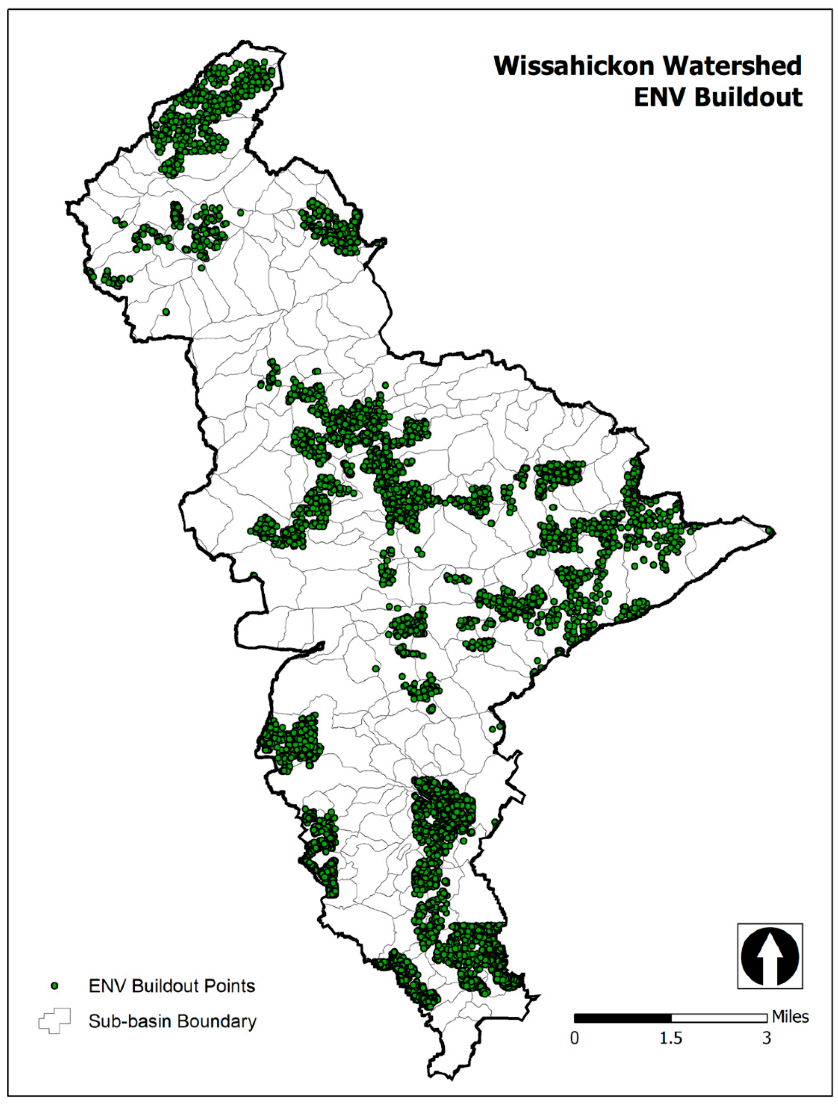
2.2.2. The Environmentally Suitable Scenario: ENV

Besides land-use (treated the same way as above), the variables of interest with respect to sustainability were slope, designation as water and floodplains, proximity to train stations and bus stops, proximity to points of interest, and proximity to parks and open spaces. Slope was based on a digital elevation model (DEM). The ArcGIS Slope tool used on the WCW-clipped DEM generated a set of values that were then reclassified. Again using the Natural Breaks classification, 5 was assigned to the lowest slope and 1 to the highest. The process of preparing the water and floodplains raster was more complicated. A buffer of 50 feet was placed on the streams file. To the streams, floodplains, and wetlands layers a field named water type was added. The field was populated with 100-year, 500-year, floodway, wetland, stream, and outside. The water-related files (100-year floodplain, 500-year floodplain, floodway, stream buffer, wetlands) were merged, and the Union tool brought them into the WCW boundary layer. A raster grid was created using water type as the value field, and it was reclassified to floodway, stream buffer, and wetlands as 0, 100 years as 1, 500 years as 2, and everything else as 5.

The “proximity to” variables (train stations and bus stops, points of interest, and parks and open spaces) were all treated the same way. The different feature classes were merged, Euclidean distance was used for distances made to be within the WCW boundary, the distance values were reclassified using the Natural Breaks classification, and 5 was given to the closest and 1 to the farthest away. Points of interest were schools, places of worship, hospitals/clinics, employment centers, and colleges/universities. The parks were from Montgomery County and Philadelphia. Open spaces were in a protected open space layer.

The criteria represented by the reclassified rasters were given weights. The weights were based on a survey of municipal officials, planners, and nonprofit environmental advocacy groups. The survey was distributed in 2016 to 42 municipal officials and Environmental Advisory Council volunteers, of which 31 responded with complete surveys. Average weights for each criterion suggested by survey participants were calculated for the suitability analysis. The weights were proximity to train stations and bus stops (23%), water and floodplains (17%), slope (16%), land-use (16%), proximity to parks and open spaces (16%), and proximity to points of interest (12%).

2.3. Economic and Environmental Impact Analyses

The overall profitability of each scenario was determined by the distribution of buildings in the zip codes, which was based on the suitability analyses combined with the CommunityViz Scenario 360 buildouts. Statewide shapefiles of zip codes and census tracts were clipped in ArcGIS to the WCW. Spatially joining the clipped zip codes with the buildings placed by the Buildout Wizard according to profitability yielded the number of buildings in each scenario in each zip code. Using profit per square meter (PSM) as the measure, the PSM in each zip code was weighted by the buildings placed in that zip code as a percent of all buildings placed in each scenario. The weighted sum of the PSM in all zip codes was the Weighted PSM or WPSM.

The environmental effects of the location of residential development in the WCW are expressed below in terms of additional air and greenhouse emissions resulting from automobile use by new residents in the zip codes (ECON) and census tracts (ENV), and water quality changes caused by new residents in the watershed’s sub-basins (ECON, ENV). Spatially joining the clipped census tracts with the buildings placed by the Buildout Wizard in ECON and ENV yielded the number of buildings in each scenario in each census tract.

The Greenhouse Gases, Regulated Emissions, and Energy Use in Transportation (GREET1 2018) Program [55] was used to generate energy use, criteria air pollution emissions, and greenhouse gas emissions for a user-chosen, generic, passenger hybrid automobile that uses spark ignition (SI) and internal combustion with California reformulated gasoline along with an electric motor (ICEV). The data for vehicle kilometers travelled (VKT) were converted from miles travelled, available from the Bureau of Transportation Statistics at the US Department of Transportation [56]. The data were assembled from the National Highway Travel Survey, and were available for census tracts by state. The VKT in each census tract was weighted by the buildings placed in that census tract as a percentage of all buildings placed in each scenario. The weighted sum of the VKT in all census tracts was the Total VKT or TVKT for each scenario.

Several authors (e.g., [57,58,59,60,61]) used a composite water quality index (WQI) to characterize a variety of water bodies. Brown et al. [61] used an iterative Delphi survey process among experts to determine those components thought to be the most relevant for assessment, and to assign relative weights to those chosen. Walsh and Wheeler [60] noted that this approach, with a few enhancements, was still being used by the US EPA, state governments, and other countries. Of the four alternative forms of the WQI discussed by those authors, the arithmetic mean (additive form) and a variant of the geometric mean (multiplicative form) were chosen for this work. The former does not revert to a zero index value when any of the parameter values is zero. When the parameter values are not zero, the presence of a low parameter value affects the index more acutely in the latter. Lumb et al. [58] noted that these forms of the WQI are the most popular. Important criteria that they both satisfy are: ease of use, a reasonable balance between oversimplification and technical complexity, and applicability for showing trends over time, comparisons of different locations, and public information purposes [60].

The effects of residential development on water quality (WQ) in the WCW involved certain biological, chemical, and physical components. The data on the values of these components were provided by the Philadelphia Water Department [62], though some of the data were collected by the US Geological Survey, the PA DEP, Temple University’s Center for Sustainable Communities, and the Wissahickon Valley Watershed Association. The health of the biological communities in the WCW was represented by the Index of Biotic Integrity (IBI) computed for benthic macroinvertebrates [63]. Some index values of these communities were also provided by the PWD [62].

To estimate the differences the two development scenarios had on WQ and IBI, a division of the WCW into 213 sub-basins was used. Spatial join was used in ArcGIS 10.6 to find the housing units in each sub-basin in both scenarios. The sub-basins that drained into the monitoring stations listed in Table 6 were given the WQI and IBI values of that station. The number of housing units placed in those sub-basins, as a percentage of all units placed, was used as a weight on the WQI and IBI for each monitoring station in each scenario. Summing over the monitoring stations yielded the additive form of the weighted WQI (WWQI) and weighted IBI (WIBI) for each scenario. Equations (2) and (3) show the forms of these indices. Equation (4) shows the geometric form of the WWQI. As noted above, this form is particularly sensitive to a low or missing value of any parameter.

$${\mathrm{WWQI}}_{add}={{\displaystyle \sum }}_{\mathrm{i}=1,2,4}^{10}{\mathrm{w}}_{\mathrm{i}}{\ast \mathrm{WQI}}_{\mathrm{i}}.$$

(2)

Station i = 3 did not have enough parameter data to be included.

$$\mathrm{WIBI}={{\displaystyle \sum }}_{\mathrm{i}=2,3,5}^{10}{\mathrm{w}}_{\mathrm{i}}\ast IB{I}_i.$$

(3)

Stations i = 1,4 did not have enough parameter data to be included.

$${\mathrm{WWQI}}_{mult}={{\displaystyle \prod }}_{i=1}^{9}WQ{I}_i^{w_i}.$$

(4)

Station i = 10 received zero buildings in both scenarios. A zero value for WQI₁₀ would have given the entire WQI a zero value; this was avoided by deleting it.

As the data for the various impacts were reported for different spatial units, Spatial Join in ArcGIS 6.2 was used to covert building counts among the zip codes, census tracts, and sub-basins.

2.4. Ecosystem Goods and Services Valuation

An important consequence of the environmental impacts is the effect on the ecosystems within the WCW, and their value. Air emissions and greenhouse gas emissions (indirectly), and water quality and biotic integrity changes will have effects on local ecosystems. The land-use polygons in Figure 2 of concern for ecosystem effects are recreation, water, and wooded.

While the determination of the values of ecological parameters is important, “…measuring or assessing ecosystem services requires moving beyond ecological measures that are not explicitly linked to human benefits to make causal connections between changes in a natural system to the ecosystem services outcomes that are valued by people” [64] (Section 1, p. 14). Ringold et al. [65] stressed that analysts should differentiate between “intermediate” biophysical elements and “final” ecosystem goods and services (FEGS). The latter must be tied to beneficiaries. Formal classifications of the FEGS have been the subject of considerable effort over the past few decades, often mimicking the North American Industrial Classification System (NAICS). Examples are [66,67,68]. The generally-accepted broad categories of FEGS are provisioning, regulation, cultural, and supporting.

Table 5. Impacts on final ecosystem goods and services (FEGS) and beneficiaries.

Impacts of Residential Development	FEGS Category	FEGS via a More Benign Scenario	Beneficiaries	Benefit
Stormwater runoff added to baseflow; streambank erosion; nutrient and sediment buildup	Provisioning	Cleaner water supply	Philadelphia Water Dept. and drinking water consumers	Reduced increase in water-treatment costs
Auto traffic air and greenhouse emissions; air pollution deposition	Regulation	Higher air pollution mitigation; higher greenhouse gas mitigation; lower deposition	Downwind citizens; downstream citizens; nearby residents	Reduced health problems; reduced property damage
Degradation of the local natural environment	Cultural *	Reduced degradation during nature visits	Visitors and nature-lovers	Reduced loss of value
Negative feedback loops	Supporting	Natural biological, chemical, and physical cycles	All the above	???

* This is taken to mean all of Residential; Recreational; Inspirational; and Learning and Non-Use.

links the impacts of the more benign scenario to ultimate benefits to classes of beneficiaries. In terms of land-use change, development in the residential polygons affects the structure and function of the elements within the recreation, water, and wooded polygons.

The application of the sequential elements of the methodology led to the outcomes discussed in the next section.

3. Results

The buildouts using the CommunityViz 5.2 Scenario 360 followed the ArcGIS 6.2 suitability analyses using profitability and sustainability criteria, respectively. As noted above, these results were examined in terms of profit, air pollution, and greenhouse gas emissions, and water-quality in the WCW. The value of ecosystem goods and services can be affected by the environmental impacts.

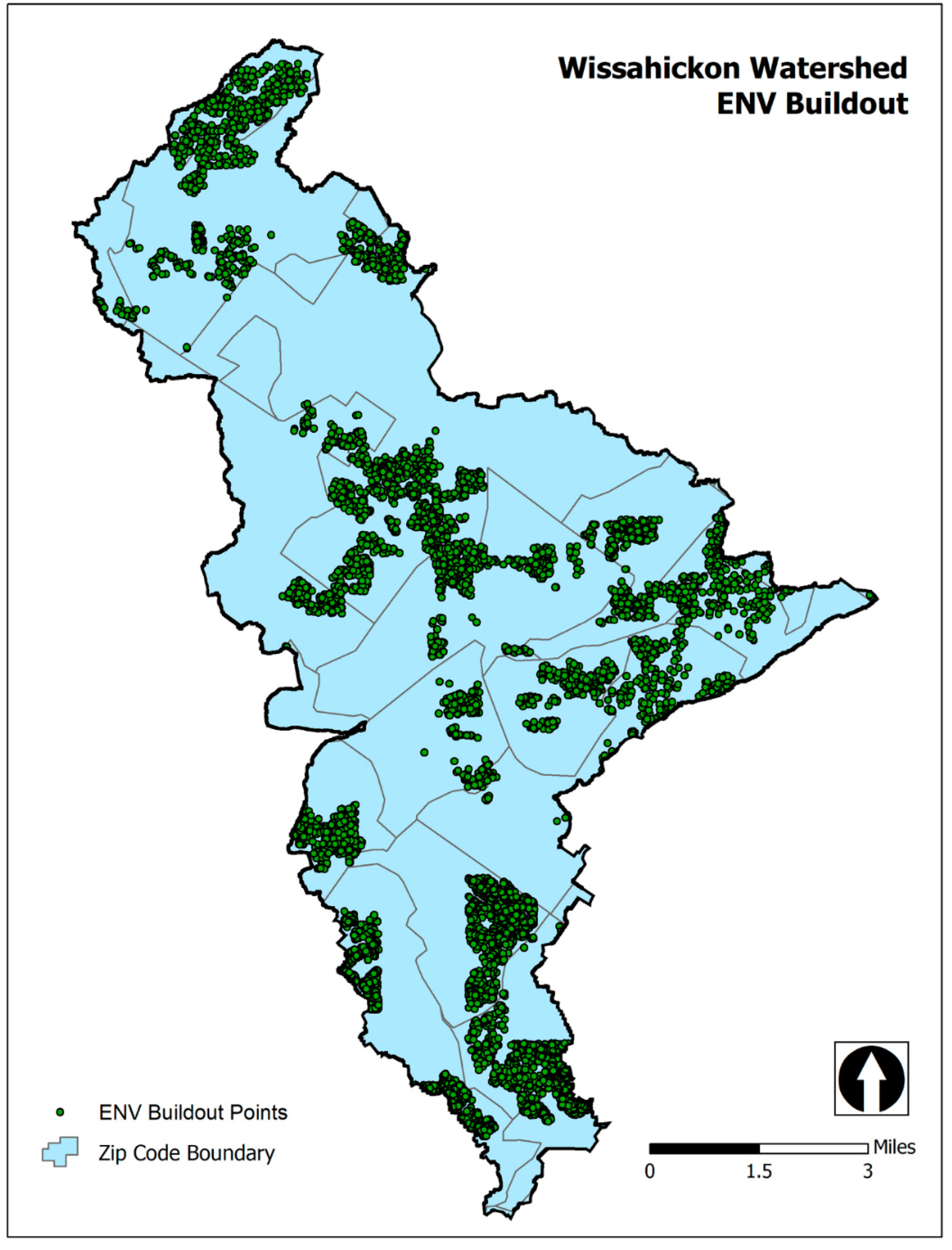
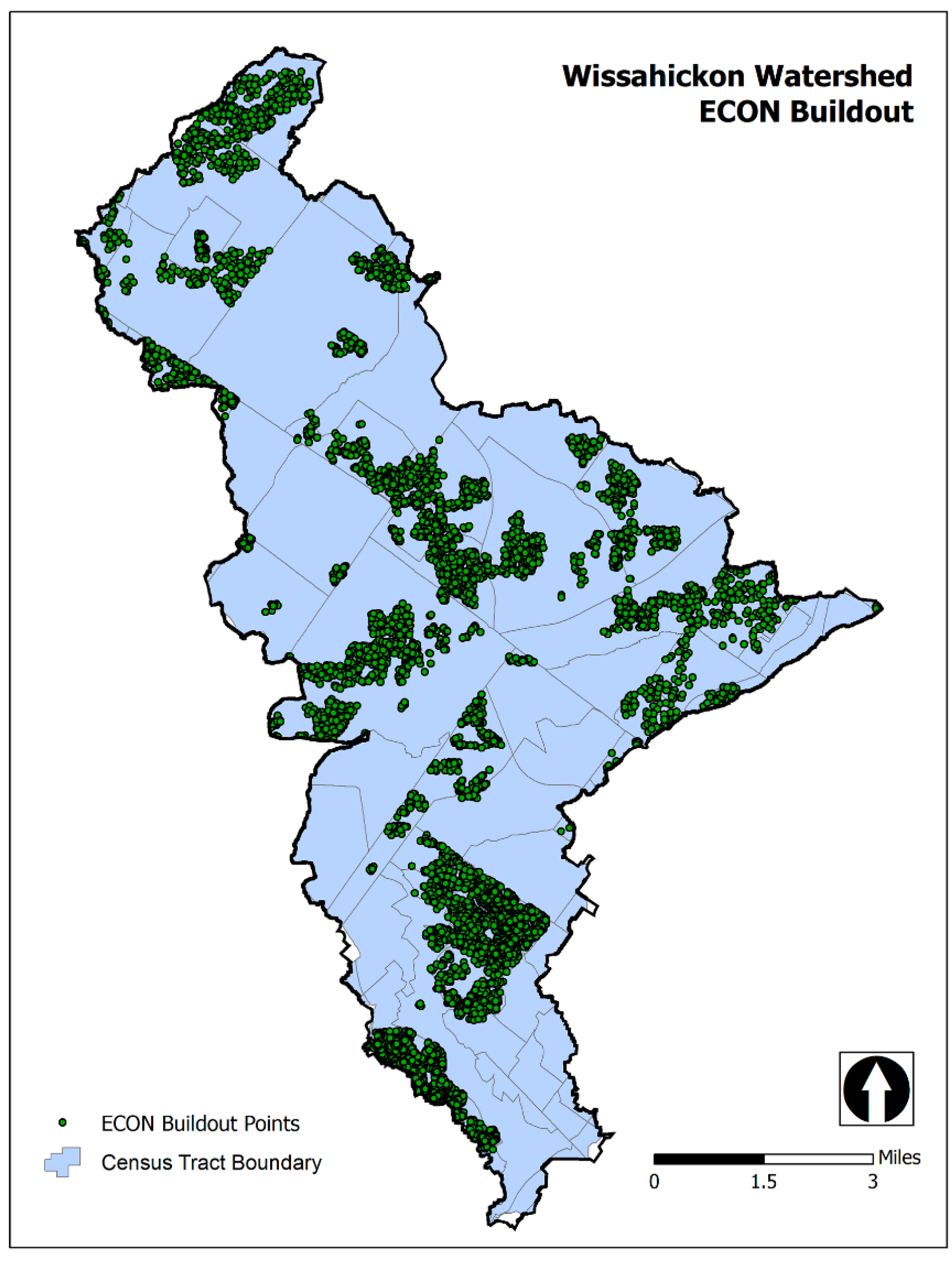
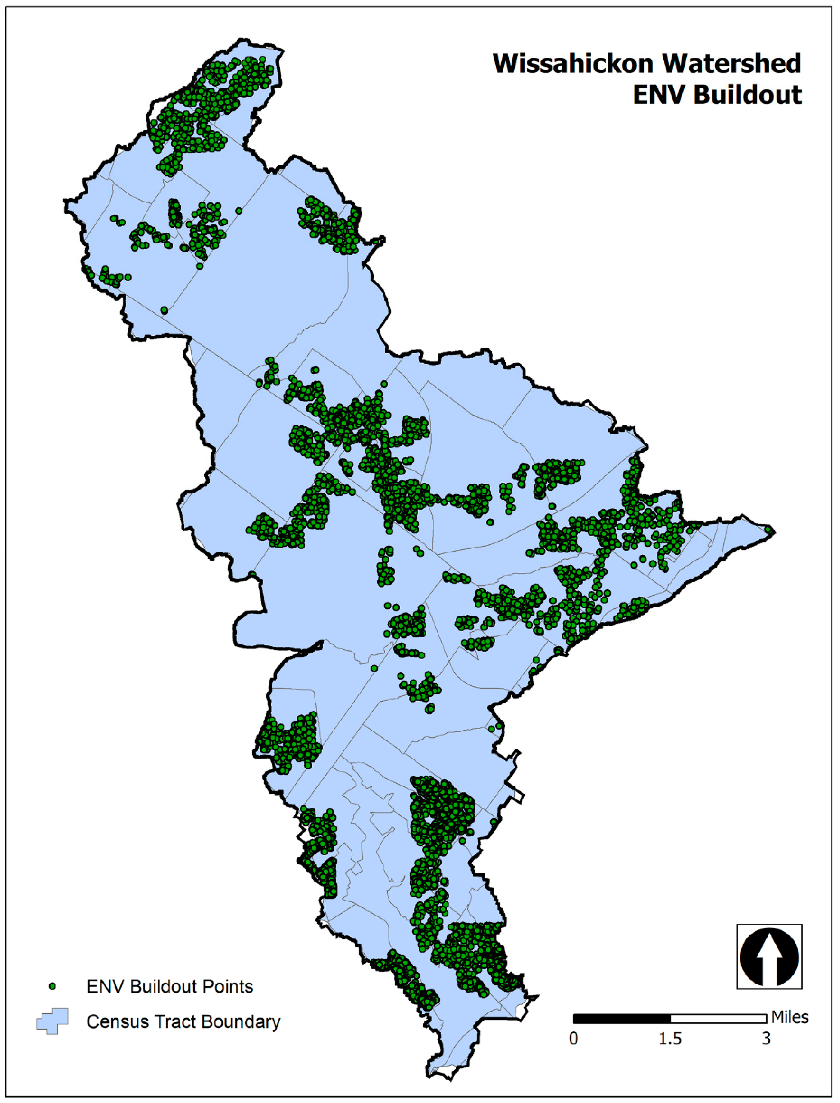
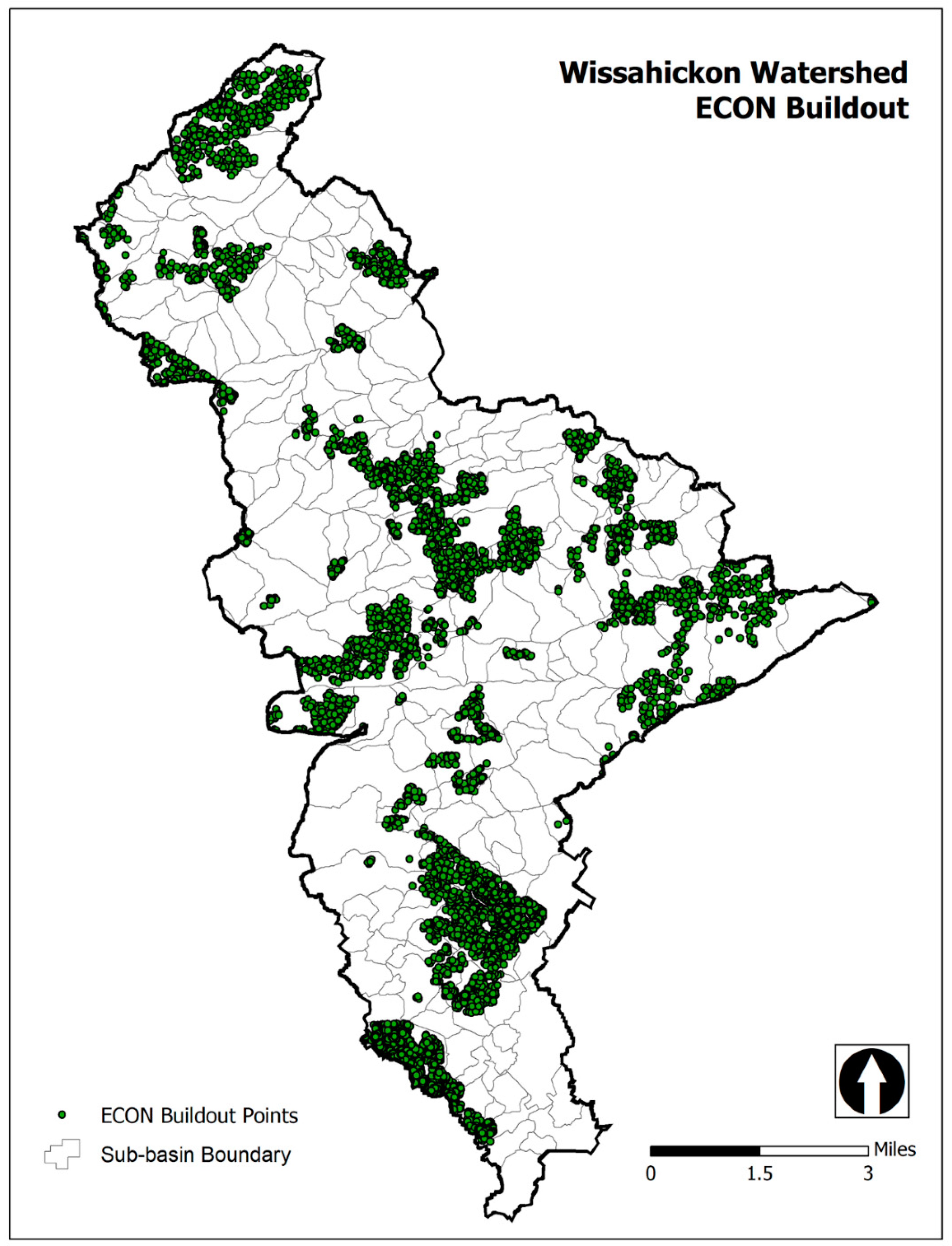
3.1. Housing Location in the ECON and ENV Scenarios

Figure 3 presents the range of suitable areas according to the criteria in the ECON scenario.

Figure 4 contains the distribution of buildings across the zip codes in the ECON scenario.

Figure 5 shows the range of suitable areas according to the criteria in the ENV scenario.

Figure 6 displays the buildings in the zip codes for the ENV scenario.

Figure 7 displays the buildings in the census tracts for the ECON scenario.

Figure 8 shows the distribution of the buildings in the census tracts for the ENV scenario.

The energy use and emissions data are given in

Table 6. Energy use and emissions from GREET1 2018.

GREET WTW Run with Vehicle SI ICEV CA Gasoline
					Total ECON	Total ENV
Name	WTP	Operation	WTW	Total Units	405,885 VKT	394,554 VKT
Total Energy (kJ/km)	704.97	2819.25	3524.22	MJ	1,430,429.50	1,390,496.52
Fossil Fuel (kJ/km)	3286.34	0	3286.34	MJ	1,333,874.25	1,296,636.78
Coal Fuel (kJ/km)	45.67	0	45.67	MJ	18,537.10	18,019.60
Natural Gas Fuel (kJ/km)	439.89	0	439.89	MJ	178,546.54	173,562.10
Petroleum Fuel (kJ/km)	2800.62	0	2800.62	MJ	1,136,730.10	1,104,996.26
Renewable (kJ/km)	229.25	0	229.25	MJ	93,051.03	90,453.34
Biomass (kJ/km)	222.34	0	222.34	MJ	90,242.61	87,723.32
Nuclear (kJ/km)	8.73	0	8.73	MJ	3544.56	3445.61
VOC (g/km)	0.08	0.08	0.17	g	68.07	66.17
CO (g/km)	48.21	1.68	1.73	g	700.84	681.28
NOx (g/km)	0.12	0.07	0.20	g	80.67	78.42
PM10 (mg/km)	12.05	3.36	15.40	mg	6252.14	6077.60
PM2.5 (mg/km)	8.82	2.97	11.79	mg	4784.91	4651.33
SOx (g/km)	0.08	0.001	0.08	g	32.77	31.86
CH4 (g/km)	0.30	0.01	0.31	g	126.05	122.53
CO2 (kg/km)	0.05	0.20	0.25	kg	100.84	98.03
N2O (mg/km)	7.49	4.73	12.22	mg	4958.86	4820.42
VOC Urban (g/km)	0.05	0.07	0.11	g	45.38	44.11
CO Urban (g/km)	0.01	1.38	1.39	g	562.19	546.49
NOx Urban (g/km)	0.02	0.06	0.08	g	32.77	31.86
PM10 Urban (mg/km)	3.36	2.75	6.11	mg	2480.69	2411.44
PM2.5 Urban (mg/km)	2.72	2.43	5.16	mg	2092.45	2034.04
SOx Urban (mg/km)	20.99	1.00	21.99	mg	8924.43	8675.29
CH4 Urban (mg/km)	8.80	4.40	13.20	mg	5357.18	5207.62
CO2 Urban (kg/km)	0.03	0.17	0.19	kg	78.15	75.97
N2O Urban (mg/km)	0.30	3.88	4.18	mg	1696.65	1649.28

, where WTP, WTW, and VKT are well-to-pump, well-to-wheels, and vehicle kilometers travelled, respectively. The air emissions are volatile organic compounds (VOC), carbon monoxide (CO), nitrogen oxides (NO_x), particulate matter with 10- and 2.5-microns diameter (PM₁₀, PM_2.5), and sulfur oxides (SO_x). The greenhouse gas emissions are methane (CH₄), carbon dioxide (CO₂), and nitrous oxide (N₂O).

The TVKT are listed in the headings of the right-most columns of Table 5. When multiplied by the TVKT, the energy use and emissions results listed in those columns were generated. The distribution based on sustainability had a 3% lower TVKT.

The ECON buildings in the WCW sub-basins are shown in Figure 9. The ENV buildings in the WCW sub-basins are shown in Figure 10.

The values of the WQI, WWQI, IBI, and WIBI for the monitoring stations at which the most data were collected are given in

Table 7. Water quality index and index of biological integrity.

Station	WQI (add)	WQI (mult)	IBI
WS2041	73.57	69.38	*
WS1850	58.43	52.42	23.16
WS1371	*	*	24.84
WS1317	69.38	67.66	*
WS1140	62.32	56.12	26.27
WS1075	71.55	63.21	21.21
WS754	61.9	57.19	20.17
WS405	64.4	60.69	17.75
WS076	71	38.39	20.17
WS005	80.82	34.95	17.75

An * indicates that the index at the top of the column was not computed for that station.

. The names of the stations reflect the number of Creek-miles northward from the mouth of the Wissahickon Creek in the south of the WCW. For example, WS1075 is 10.75 miles from the mouth.

Table 8. Weighted water quality index (WQI) and Index of Biotic Integrity (IBI).

Station	%-ECON Bldgs	%-ENV Bldgs	WWQI (add) ECON	WWQI (add) ENV	WWQI (mult) ECON	WWQI (mult) ENV	WIBI ECON	WIBI ENV
WS2041	0.078	0.082	5.72	6.04	5.39	5.70	*	*
WS1850	0.036	0.027	2.11	1.60	1.89	1.44	0.84	0.64
WS1371	0.060	0.059	*	*	*	*	1.50	1.46
WS1317	0.040	0.041	2.80	2.87	2.73	2.80	*	*
WS1140	0.087	0.100	5.40	6.25	4.86	5.63	2.28	2.63
WS1075	0.116	0.079	8.32	5.62	7.35	4.96	2.47	1.67
WS754	0.124	0.134	7.70	8.31	7.12	7.67	2.51	2.71
WS405	0.231	0.220	14.88	14.15	14.03	13.33	4.10	3.90
WS076	0.227	0.257	16.13	18.22	8.72	9.85	4.58	5.18
Total	1.000	0.999	63.05	63.05	52.08	51.38	18.27	18.18

An * indicates that the index at the top of the column was not computed for that station.

shows the weighted values of the indices using as weights the percentage of all housing units placed in each of the sub-basins.

Table 9. Overall comparison of ECON and ENV.

Indicator	ECON	ENV	Assessment	ECON-ENV
WPSM($)	22.23	10.82	Higher is better	11.41
TVKT *	405,885	394,554	Lower is better	11,331
WWQIadd	63.052	63.054	Higher is better	−0.002
WWQImult	52.08	51.38	Higher is better	0.70
WIBI	18.18	18.27	Higher is better	−0.09

* This is a proxy for air and greenhouse emissions.

displays the comparison of the two scenarios in terms of the major indicators discussed above. The bold number indicates the scenario with the better assessment value.

The ECON scenario generated a weighted profit per square meter of $22.23. The ENV scenario resulted in 394,554 weighted vehicle kilometers travelled, an weighted additive water quality index of 63.054, a weighted multiplicative water quality index of 51.38 and a weighted index of biological integrity of 18.27. Each of these numbers were better for each criterion than those generated in the other scenrio.

3.2. The Value of Ecosystem Goods and Services

In its provisioning mode, the Wissahickon Creek enters the Schuylkill River near the Queen Lane intake at the left-bottom of the WCW in Figure 1. It makes up about 10 percent of the water that will become drinking water [69]. The Queen Lane Water Treatment Plant processes 70 million gallons per day. The current average price of a gallon of water in Philadelphia is $0.009. The revenue generated is $630,000 per day, or $229,950,000 per year. Ten percent of that revenue, $22,995,000, comes from the Wissahickon Creek. The provision of water from the creek is valued at almost $23 million per year. Despite the potential redistribution of rainwater between ground storage and surface runoff, the quantity of water provided by both development scenarios was thought to be the same. Since the WWQI in both forms for the ECON and ENV scenarios was virtually the same, neither has a substantial advantage in terms of avoided treatment costs due to lower water quality.

As Wissahickon Creek is a stocked trout fishery, the value of recreational fishing can be estimated in a general way. Schneck [70] listed estimates of the numbers of anglers, their spending, and the economic ripple effects of that spending for pre-2018 PA congressional districts. The pre-2018 districts that intersected the WCW were PA-2, PA-7, and PA-13. Area-wise, the WCW made up approximately 17%, 10%, and 25% of these districts. Assuming that anglers are uniformly distributed in the districts, then the WCW in each of these districts contains 10,085, 11,966, and 9872 anglers who spend $2.12 million, $2.52 million, and $2.09 million per year, respectively. The total, $7 million, can be attributed to angling the Wissahickon Creek.

In 2018, the Wissahickon Valley Watershed Association (WVWA) received $3.5 million in revenue from 1236 members/individual donors. Volunteers contributed 4147 hours. Since roughly 5% of the revenue was from investments, 95% of its revenue, $3.325 million, was donated by concerned individuals and organizations [71]. The Friends of the Wissahickon (FOW) has more than 3000 members. It received $1.074 million and 12,617 volunteer hours [29]. The sum of the revenue of these organizations, $4.4 million, and the value of the sum of volunteer hours at the $7.25/hour US federal minimum wage, $121,539, will be taken as a minimum estimate of the value that beneficiaries ascribe to the non-provisioning and non-angling FEGS (e.g., inspiration from nature walks, environmental education) associated with the WCW. The total value is $4.52 million. The areas in the WCW overseen by both groups are open to the public, and visits by these beneficiaries adds value to the WCW FEGS. The sum of water revenue, angling expenditures, and organization contributions is $34.25 million.

4. Discussion

The WCW intersects with 26 zip codes. That the ECON scenario generated a better WPSM outcome is largely due to its substantially larger housing placement in the zip codes of Fort Washington (19034) and Blue Bell (19422) in the suburbs, and the Chestnut Hill (19118) section of Philadelphia. A higher placement also occurred in Roxborough (19128) with a negative profit/m², but it was outweighed by the above higher-profit areas. The ENV scenario placed considerably more housing in relatively lower-profit Glenside (19038), Oreland (19075), and Willow Grove (19090) in the suburbs and Germantown (19144) in Philadelphia. The ENV scenario placed more housing in higher-profit suburban Lafayette Hill (19444) and North Wales (19454), but each comprised a small percentage of the total housing placed in that scenario.

The WCW is covered by 86 census tracts. The ENV scenario placed many more buildings than ECON in 18 tracts that had an average VKT of 53.49. The ECON scenario placed many more buildings in 11 tracts that had an average VKT of 64.86. The ENV scenario generated fewer VKT, and its resulting energy use, air pollution, and greenhouse gas emissions were lower.

The 213 sub-basins that comprised the WCW were linked by their locations to 10 monitoring stations. The percentage difference in housing distribution by ECON and ENV was greatest for those sub-basins draining into stations WS1075 and WS076. At WS1075, ECON placed 4% more housing, and WQI_add was 71.55, WQI_mult was 63.21, and the IBI was 21.21. These are relatively high. At WS076, ENV placed 3% more housing. WQI_add was 71.00, WQI_mult was 38.39, and the IBI was 21.17. Except for WQI_mult, these are relatively high. Given that the distribution in the sub-basins draining into the other stations was about the same, the WQI in both forms and the WIBI are very close. That the ECON scenario had a better WQI_mult is a bit of an anomaly.

4.1. Similarities and Differences with Previous Work

The approach and results of this work contain many similarities with the previous literature, especially the goal in Hudson [4] of preserving natural capital, and the watershed scale of analysis. The present study is similar to Guo et al. [15] in that it created scenarios at the watershed scale with sub-catchments differentiated in a SWMM model. It is different in that it assumed that uniform housing units (without LID fixes) placed in particular sub-catchments would take on the water quality values associated with that catchment. Runoff coefficients were not estimated here. As with Hasanzadeh et al. [2], Saiz [3], and others, it used GIS and related software to manipulate the spatial data. However, it involved the supply of housing units placed in criteria-suitable areas within precise municipal zoning codes. It shares with Almeida et al. [14] the use of the GREET 2018 model, and with Nesheim and Barkved [18] and Fan and Shibata [22] inclusion of the ecosystem service of water provision. The current approach has much in common with Berg and BenDor [20], in particular, planning for watershed protection. The work also shares the concern for the urban–suburban divide with Hanlon [10] and Koshkar et al. [7].

The present work also shares the WQI approach of Sánchez et al. [57], Lumb et al. [58], Tyagi et al. [59], Walsh and Wheeler [60], and Brown et al. [61]. Given the complexity of the water-quality issue, a composite score can be useful if applied consistently across scenarios. One caveat may be the regional applicability of an index based on nationally-uniform weighting parameters. Of course, sensitivity analysis can remedy this shortcoming.

The techniques used in this work intersect the most with Sorrentino et al. [11] and Sorrentino et al. [12]. The former study generated two scenarios, namely trend and suitable, of housing location in the Pennypack Creek Watershed (PCW). The trend scenario allowed housing in only those municipalities with positive population projections made by DVRPC. The result was housing only placed in certain suburban municipalities and not in the City of Philadelphia. The suitable scenario placed housing according to sustainability criteria, and many housing units were placed in the City. While profitability was not analyzed, most environmental impacts were significantly lower for the suitable scenario. An anomaly occurred with respect to water quality. The trend scenario had higher overall water quality than the suitable scenario. Broad impacts on ecosystem services valuation were applied via benefits transfer.

Sorrentino et al. [12] used the same approach as in this paper to examine the impacts of four residential development scenarios within the PCW. Two scenarios were built on economic suitability and two on environmental suitability. In each category, one scenario followed only municipality zoning ordinances, while the other used an author-generated uniform zoning code. No effort was made to compute ecosystem services values. Except for the environmental suitable scenario with uniform zoning (ENV-UNI), the scenarios followed the DVRPC projection of zero growth for Philadelphia. ENV-UNI had the lowest profit, the lowest air pollution and greenhouse gas emissions, the highest biological integrity, but only the second-highest water quality. The authors concluded that it was quite likely that profitability and sustainability did not occur together.

The results of the present work on the WCW jibe with those of Sorrentino et al. [12] in that profit in the sustainable scenario was remarkably lower, but differ with respect to the environmental impacts. The environmental impacts of the two scenarios in the WCW were quite similar. This might lead an analyst to question whether profitability and sustainability cannot be satisfied simultaneously.

4.2. Effects on Ecosystem Goods and Services

The attempt to assign value to the ecosystem goods and services provided by the WCW fell short of the detail required by the National Ecosystem Services Partnership [64], Ringold et al. [65], Landers, D. and A. Nahlik [66], US EPA [67], and the European Environment Agency [68]. One reason, as noted by Lyle [37], is the magnitude of the task of specifying the ecological processes in detail. A second reason is that the search for valuation tools to process data at the WCW scale came up empty. Future research collaboration with ecologists and others will help in creating a more detailed specification. A soon-to-be-released updated version of the ARIES valuation software [72] will be a step toward solving the tools problem.

5. Policy Implications and Conclusions

Residential development will continue in the WCW if it is profitable and there is space for it, all others things constant. Demand and supply in the housing market can interact with local governments having control over location through the zoning designated for each area, though Sorrentino et al. [11], Sorrentino et al. [12], Berg and BenDor [20], and others proposed that regional/watershed planning may be better. Since the ECON scenario generated 17% higher profit, 3% more air pollution, and greenhouse gas emissions and was effectively equal to ENV in water-quality degradation, it may be seen to be preferred in a monetary view of societal welfare.

If, on the other hand, government officials become quite vigilant in their efforts to upgrade the air quality and lower greenhouse gas emissions in the WCW, then the ENV scenario may be their choice. That officials should become more vigilant is evidenced in part by a US-wide report by the American Lung Association [73], which was reduced to the Philadelphia metro region in American Lung Association [74]. According to the latter, the region experienced an increase in ozone smog from 2015 to 2017 after decades of decline. While there has been an improvement in small-particle pollution, the region was still ranked among the worst in the US. The smog problem is exacerbated by higher temperatures, possibly due to climate change. The most vulnerable populations are people with respiratory ailments, children, and older adults. In the WCW, the components of smog from Table 5 (VOC, NO_x, and PM_2.5) will be 3% higher in the ECON scenario. The ENV scenario may be strictly preferable due to the negative air-quality trend and the prediction of a warmer and wetter climate.

As noted above, the Wissahickon Creek has been designated an impaired stream. This is essentially due to wastewater treatment plant discharges during low base-flow and stormwater runoff. The US EPA established two Total Maximum Daily Loads (TMDLs) for impaired streams in the WCW in 2003 based on PA DEP assessments under the US Clean Water Act, Section 303(d), with respect to siltation and the following nutrients—ammonia nitrogen, nitrate-nitrite, orthophosphate, and carbonaceous biological oxygen demand [75]. The EPA proposed a Total Phosphorus TMDL in 2015 as a supplement to the 2003 Nutrient TMDL to address nuisance algae [76]. Given the strictness of the 2015 TMDL, “The municipalities in the Wissahickon Creek Watershed have joined together to form a coalition of towns and sewer authorities working with the … PA DEP and the … US EPA to address our impaired stream health. This coalition, called the Wissahickon Clean Water Partnership, will be working on a plan over the next two years to collaboratively ‘Own the Solution’ for a cleaner Wissahickon Creek [77].” Further evidence of the need for improvement is the PA Fish and Boat Commission [78] advisory that people limit their consumption of freshwater fish from PA waters to one eight-ounce (before cooking) meal per week.

Several regulatory and/or economic policy tools are available to accomplish general air quality and general water quality goals, though these have not been implemented for greenhouse gasses at the federal level in the US. The current executive branch of the federal government has moved to reduce or eliminate environmental regulations. In the face of this, many US states and local regions have acted to offset or work around these reductions. Municipalities in the WCW have several means to encourage the ENV scenario with respect to air and greenhouse emissions, perhaps mimicking the collaboration involving the Clean Water Partnership [77].

Zoning restrictions can directly influence residential development, while transportation fees and various impact fees on developers can influence development by changing the relative financial returns of various options within municipalities [79]. In a watershed-wide approach, municipalities can agree not to compete by offering incentives for developers to provide the ECON scenario at the expense of foregone environmental benefits of the ENV scenario. They can also agree to provide regulatory monitoring within an adaptive management system.

In conclusion, the small differences in the environmental impacts may seem to indicate that policymakers should limit intervention and let the housing market generate the ECON scenario within existing zoning and other regulations. As noted above, however, trends in air pollution and greenhouse gas emissions are heading in the wrong direction. Increased impervious surfaces exacerbate stormwater problems. The need to reverse these trends, regardless of the small differences, should prompt policy action. The policy alternatives discussed above are in practice in various locations in PA, and can be implemented in others.

With respect to water quality, the Wissahickon Creek needs improvement independent of whether the ECON or the ENV scenario would eventually unfold. Policy incentives also exist to make this happen, and an encouraging element in the resolution of these problems is the cooperation of the public WCW organizations in the Clean Water Partnership. Another positive component in the task of improving the Creek is the continuous improvement approach taken by the WVWA [71] and the FOW [29].

Further research on the effects of residential development in the WCW will pursue more detail on the ecological processes that occur in the Creek and its surroundings. As more detail is generated, the effects on the FEGS the WCW supplies will become more precise. More detailed work on the value of the FEGS is anticipated. Additional insights can be gained by choosing alternative assumptions about the automobile/fuel combinations in the GREET program, and other options in some parts of the CommunityViz Scenario 360 Buildouts. Branching out from the housing buildout approach may involve the conservation districts, and transit-oriented, mixed-use, and infill development discussed by Göçmen et al. [8]. The downsizing of dwellings of Sandberg [5], the “backcasting” of Musse et al. [6], the “eco-districts” of Stachuro [9], the Blue-Green Infrastructure network approach of Ahmed et al. [21], and the expanded business model of Dunphy et al. [13] can help inform future planning and put the two scenarios described above into a broader perspective.

With this new knowledge, the ecological–economic argument for natural capital preservation in the name of sustainability will gain more momentum as urban agglomerations continue to grow.

References

1. United Nations (UN). World Urbanization Prospects 2018. Department of Economic and Social Affairs, Population Division. Available online: https://population.un.org/wup/ (accessed on 24 February 2019).
2. Hasanzadeh, K.; Kyttä, M.; Brown, G. Beyond Housing Preferences: Urban Structure and Actualisation of Residential Area Preferences. Urban Sci. 2019, 3, 21. [Google Scholar] [CrossRef]
3. Saiz, A. The Geographic Determinants of Housing Supply. Q. J. Econ. 2010, 125, 1253–1296. [Google Scholar] [CrossRef]
4. Hudson, B. Realigning Metrics of Economic Well-Being in Residential and Commercial Development through Sustainable Land Use Planning. Washburn Law J. 2015, 54, 575–584. [Google Scholar]
5. Sandberg, M. Downsizing of Housing: Negotiating Sufficiency and Spatial Norms. J. Macromktg. 2018, 38, 154–167. [Google Scholar] [CrossRef]
6. Musse, J.; Homrich, A.S.; De Mello, R.; Carvalho, M.M. Applying backcasting and system dynamics towards sustainable development: The housing planning case for low-income citizens in Brazil. J. Clean. Prod. 2018, 193, 97–114. [Google Scholar] [CrossRef]
7. Khoshkar, S.; Balfors, B.; Wärnbäck, A. Planning for green qualities in the densification of suburban Stockholm—Opportunities and challenges. J. Environ. Plan. Manag. 2018, 61, 2613–2635. [Google Scholar] [CrossRef]
8. Göçmen, Z.A.; LaGro, J.A., Jr. Assessing local planning capacity to promote environmentally sustainable residential development. J. Environ. Plan. Manag. 2016, 59, 1513–1535. [Google Scholar] [CrossRef]
9. Stachuro, E. Sustainable Housing Environment and Its Impact on Consumption Patterns. Kons. Rozwój. 2014, 3, 61–72. [Google Scholar]
10. Hanlon, B.; Airgood-Obrycki, W. Suburban revalorization: Residential infill and rehabilitation in Baltimore County’s older suburbs. Environ. Plan. A Econ. Space 2018, 50, 895–921. [Google Scholar] [CrossRef]
11. Sorrentino, J.; Meenar, M.; Flamm, B. Suitable housing placement: A GIS-based approach. Environ. Manag. 2008, 42, 803–820. [Google Scholar] [CrossRef]
12. Sorrentino, J.A.; Meenar, M.R.; Lambert, A.J.; Wargo, D.T. Housing location in a Philadelphia metro watershed: Can profitable be green? Landsc. Urban Plan. 2014, 125, 188–206. [Google Scholar] [CrossRef]
13. Dunphy, N.; Boo, E.; Dallamaggiore, E.; Morrissey, J. Developing a sustainable housing marketplace: New business models to optimize value generation from retrofit. Int. J. Hous. Sci. Appl. 2016, 40, 211–221. [Google Scholar]
14. Almeida, A.; Sousa, N.; Coutinho-Rodrigues, J. Quest for Sustainability: Life-Cycle Emissions Assessment of Electric Vehicles Considering Newer Li-Ion Batteries. Sustainability 2019, 11, 2366. [Google Scholar] [CrossRef]
15. Guo, X.; Du, P.; Zhao, D.; Li, M. Modelling low impact development in watersheds using the storm water management model. Urban Water J. 2019, 16, 146–155. [Google Scholar] [CrossRef]
16. Chao, P.R.; Umapathi, S.; Saman, W. Water consumption characteristics at a sustainable residential development with rainwater-sourced hot water supply. J. Clean. Prod. 2015, 109, 190–202. [Google Scholar] [CrossRef]
17. Xian, G.; Crane, M.; Su, J. An analysis of urban development and its environmental impact on the Tampa Bay watershed. J. Environ. Manag. 2007, 85, 965–976. [Google Scholar] [CrossRef]
18. Nesheim, I.; Barkved, L. The Suitability of the Ecosystem Services Framework for Guiding Benefit Assessments in Human-Modified Landscapes Exemplified by Regulated Watersheds—Implications for a Sustainable Approach. Sustainability 2019, 11, 1821. [Google Scholar] [CrossRef]
19. Azarnivand, A.; Banihabib, M.E. A Multi-level Strategic Group Decision Making for Understanding and Analysis of Sustainable Watershed Planning in Response to Environmental Perplexities. Group Decis. Negot. 2017, 26, 629–648. [Google Scholar] [CrossRef]
20. Berg, H.E.; Bendor, T.K. A Case Study of Form-Based Solutions for Watershed Protection. Environ. Manag. 2010, 46, 436–451. [Google Scholar] [CrossRef]
21. Ahmed, S.; Meenar, M.; Alam, A. Designing a Blue-Green Infrastructure (BGI) Network: Toward Water-Sensitive Urban Growth Planning in Dhaka, Bangladesh. Land 2019, 8, 138. [Google Scholar] [CrossRef]
22. Fan, M.; Shibata, H. Spatial and Temporal Analysis of Hydrological Provision Ecosystem Services for Watershed Conservation Planning of Water Resources. Water Resour. Manag. 2014, 28, 3619–3636. [Google Scholar] [CrossRef]
23. Fairmount Park Commission, Montgomery County Planning Commission, and Pennsylvania Department of Conservation and Natural Resources. (FPC, MCPC, & PA DCNR). Wissahickon Creek River Conservation Plan. 2000. Available online: http://www.phillywatersheds.org/doc/Wissahickon_RCP.pdf (accessed on 20 April 2015).
24. US Census Bureau. TIGER/Line Shapefiles 2013. 2010; Census Blocks. Available online: http://www.census.gov/geo/maps-data/data/tiger-line.html (accessed on 5 May 2018).
25. PA Department of Community and Economic Development (DCED). Governor’s Center for Local Government Services. The Comprehensive Plan in Pennsylvania, 7th ed. 2001. Planning Series #3. Available online: https://www.ckcog.com/wp-content/uploads/PADCED_Comprehensive_Plan_7th_ed.pdf (accessed on 17 July 2016).
26. McElfish, J.M., Jr. New Paths in Existing Law: Opportunities for Pennsylvania to Avoid Sprawl. Widener Law J. 2007, 16, 853–878. [Google Scholar]
27. Montgomery County, P.A. Chapter 10—Wissahickon Creek Conservation Landscape. Natural Areas Inventory Update 2007. Available online: https://www.montcopa.org/1092/Natural-Areas-Inventory-NAI-Update (accessed on 14 July 2019).
28. Miller, M. Philly Wildlife: Feral Cats, Philadelphia Parks & Recreation 2018. Available online: https://www.phila.gov/2018-01-08-philly-wildlife-feral-cats/ (accessed on 1 October 2019).
29. Friends of the Wissahickon (FOW). Connections: Annual Report 2018. 2019. Available online: http://www.fow.org/wp-content/uploads/2019/06/FOW128_2018AnnualReport_Electronic_2019_06_12_compressed.pdf (accessed on 17 July 2019).
30. Philadelphia Water Department. (PWD). Wissahickon Creek Watershed Comprehensive Characterization Report; PWD: Philadelphia, PA, USA, 2007; Available online: http://archive.phillywatersheds.org/doc/Wissahickon_CCR.pdf (accessed on 10 October 2017).
31. Delaware Riverkeeper Network. Wissahickon Creek Hit Again: DNR Calls for Environmental Accountability 2006. Available online: http://www.delawareriverkeeper.org/resources/PressReleases/Wissahickon Creek_Hit_Again_DRN_Calls_for_Accountability_6-21-06.pdf (accessed on 18 August 2019).
32. Pennsylvania Department of Environmental Protection (PA DEP). Pennsylvania Integrated Water Quality Monitoring and Assessment Report; PA DEP: Harrisburg, PA, USA, 2018; Available online: https://www.depgis.state.pa.us/2018_integrated_report/index.html (accessed on 14 June 2019).
33. Environmental Protection Agency (EPA). Wissahickon Creek TMDL; EPA: Philadelphia, PA, USA, 2003; Available online: https://boroughofambler.com/download/stormwater_management/related_documents/WissahickonTMDL_Report.pdf (accessed on 10 August 2019).
34. Temple University, Center for Sustainable Communities. Wissahickon Creek Watershed—Act 167 Plan; Montgomery County, PA, USA, 2013. Available online: https://www.montcopa.org/2264/Wissahickon-Creek-Watershed-Act-167-Plan (accessed on 16 January 2017).
35. Delaware Valley Regional Planning Commission (DVRPC). Municipal-Level Population Forecasts, 2015–2045. 2016. Available online: https://www.dvrpc.org/webmaps/popforecast/ (accessed on 27 January 2019).
36. DVRPC. Regional, County, and Municipal Employment Forecasts, 2015–2045. 2016. Available online: https://www.dvrpc.org/Reports/ADR023.pdf (accessed on 1 October 2019).
37. Lyle, J.T. The utility of semi-formal models in ecological planning. Landsc. Urban Plan. 1991, 21, 47–60. [Google Scholar] [CrossRef]
38. ArcGIS Desktop 10.6; Environmental Systems Research Institute (ESRI): Redlands, CA, USA, 2017.
39. CommunityViz 5.2.0. Scenario 360; City Explained, Inc: Lafayette, CO, USA, 2018.
40. Wheeler, S.M. Planning for metropolitan sustainability. J. Plan. Educ. Res. 2000, 20, 133–145. [Google Scholar] [CrossRef]
41. Galster, G.; Hanson, R.; Ratcliffe, M.R.; Wolman, H.; Coleman, S.; Freihage, J. Wrestling Sprawl to the Ground: Defining and measuring an elusive concept. Hous. Policy Debate 2001, 12, 681–717. [Google Scholar] [CrossRef]
42. Albouy, D.; Lue, B. Driving to opportunity: Local rents, wages, commuting, and sub-metropolitan quality of life. J. Urban Econ. 2015, 89, 74–92. [Google Scholar] [CrossRef]
43. Gibbons, S.; Machin, S. Valuing school quality, better transport, and lower crime: Evidence from house prices. Oxf. Rev. Econ. Policy 2008, 24, 99–119. [Google Scholar] [CrossRef]
44. Jim, C.; Chen, W.Y. Impacts of urban environmental elements on residential housing prices in Guangzhou (China). Landsc. Urban Plan. 2006, 78, 422–434. [Google Scholar] [CrossRef]
45. Poor, P.J.; Pessagno, K.L.; Paul, R.W. Exploring the hedonic value of ambient water quality: A local watershed-based study. Ecol. Econ. 2007, 60, 797–806. [Google Scholar] [CrossRef]
46. The Reinvestment Fund. Schools in the Neighborhood: Are housing Prices Affected by School Quality? Reinvestment Brief, Issue 6. 2009. Available online: http://www.trfund.com/tag/education/ (accessed on 22 December 2017).
47. Gill, H.L.; Haurin, D.R. User Cost and the Demand for Housing Attributes. Real Estate Econ. 1991, 19, 383–396. [Google Scholar] [CrossRef]
48. Gillen, K.C. Philadelphia House Price Indexes: Technical FAQ and Documentation; Econsult Corporation: Philadelphia, PA, USA, 2005. [Google Scholar]
49. Trulia.com. Real Estate Trends 2019. Available online: http://www.trulia.com/ (accessed on 5 June 2019).
50. Glaeser, E.L.; Gyourko, J.; Saiz, A. Housing supply and housing bubbles. J. Urban Econ. 2008, 64, 198–217. [Google Scholar] [CrossRef] [Green Version]
51. RSMeans. Construction Project Costs 2018. Available online: https://www.rsmeans.com/2018-construction-project-costs.aspx (accessed on 12 March 2019).
52. Blackley, D.M. The Long-Run Elasticity of New Housing Supply in the United States: Empirical Evidence for 1950 to 1994. J. Real Estate Finance Econ. 1999, 18, 25–42. [Google Scholar] [CrossRef]
53. Mayer, C.J.; Somerville, C. Residential Construction: Using the Urban Growth Model to Estimate Housing Supply. J. Urban Econ. 2000, 48, 85–109. [Google Scholar] [CrossRef] [Green Version]
54. Somerville, C.T. Residential Construction Costs and the Supply of New Housing: Endogeneity and Bias in Construction Cost Indexes. J. Real Estate Finance Econ. 1999, 18, 43–62. [Google Scholar] [CrossRef]
55. Center for Transportation Research. Greenhouse Gases, Regulated Emissions, and Energy Use in Transportation (GREET); Energy Systems Division, Argonne National Laboratory: Lemont, IL, USA, 2018. [Google Scholar]
56. US Department of Transportation (US DOT). Bureau of Transportation Statistics. 2017 Local Area Transportation Characteristics for Households 2018. Available online: https://www.bts.gov/latch/latch-data (accessed on 31 December 2018).
57. Sanchez, E.; Colmenarejo, M.F.; Vicente, J.; Rubio, A.; García, M.G.; Travieso, L.; Borja, R. Use of the water quality index and dissolved oxygen deficit as simple indicators of watersheds pollution. Ecol. Indic. 2007, 7, 315–328. [Google Scholar] [CrossRef]
58. Lumb, A.; Sharma, T.C.; Bibeault, J.-F. A Review of Genesis and Evolution of Water Quality Index (WQI) and Some Future Directions. Water Qual. Expo. Health 2011, 3, 11–24. [Google Scholar] [CrossRef]
59. Tyagi, S.; Sharma, B.; Singh, P.; Dobhal, R. Water Quality Assessment in Terms of Water Quality Index. Am. J. Water Resour. 2013, 1, 34–38. [Google Scholar]
60. Walsh, P.J.; Wheeler, W.J. Water quality indices and benefit-cost analysis. J. Benefit Cost Anal. 2013, 4, 81–105. [Google Scholar] [CrossRef] [Green Version]
61. Brown, R.M.; McClelland, N.I.; Deininger, R.A.; Ronald, G.T. A water quality index—Do we dare? Water Sew. Works 1970, 11, 339–343. [Google Scholar]
62. Philadelphia Water Department (PWD). Wissahickon Creek Watershed Grab Sample Data 2018. Available online: http://104.236.74.130/shiny/WCWP/ (accessed on 10 February 2019).
63. Karr, J.R. Biological integrity: A long-neglected aspect of water resource management. Ecol. Appl. 1991, 1, 66–84. [Google Scholar] [CrossRef]
64. National Ecosystem Services Partnership (NESP). Federal Resource Management and Ecosystem Services Guidebook 2014; Duke University: Durham, NC. Available online: www.nespguidebook.com (accessed on 15 March 2019).
65. Ringold, P.L.; Boyd, J.; Landers, D.; Weber, M. What data should we collect? A framework for identifying indicators of ecosystem contributions to human well-being. Front. Ecol. Environ. 2013, 11, 98–105. [Google Scholar] [CrossRef]
66. Landers, D.; Nahlik, A. Final Ecosystem Goods and Services Classification System (FEGS-CS); EPA/600/R-13/ORD-004914; US Environmental Protection Agency: Washington, DC, USA, 2013.
67. US Environmental Protection Agency. National Ecosystem Services Classification System (NESCS): Framework Design and Policy Application; EPA-800-R-15-002; US EPA: Washington, DC, USA, 2015.
68. European Environment Agency (EEA). The Common International Classification of Ecosystem Services (CICES) 2019. Available online: https://cices.eu/content/uploads/sites/8/2018/03/Finalised-V5.1_18032018.xlsx (accessed on 2 April 2019).
69. Academy of Natural Sciences (ANS). Where Does Your Drinking Water Come From? 2019. Available online: https://www.anspblog.org/where-does-your-drinking-water-come-from/ (accessed on 17 July 2019).
70. Schneck, M. How Much do Anglers in Your Area Spend on Fishing? 2018. Available online: https://www.pennlive.com/pa-sportsman/2017/03/how_much_do_anglers_in_your_ar.html (accessed on 21 July 2019).
71. Wissahickon Valley Watershed Association (WVWA). Currents Winter 2019. Available online: http://www.wvwa.org/SiteData/Own/D42F2607-062C-4A73-9A30-D37C3E1AC746/2019%20Winter%20Currents62.1.24.pdf (accessed on 17 June 2019).
72. Integrated Modelling Consortium. Artificial Intelligence for Ecosystem Services (ARIES) 2019. Available online: http://aries.integratedmodelling.org/?page_id=77 (accessed on 20 October 2019).
73. American Lung Association. State of the Air 2019. 2019. Available online: https://www.lung.org/assets/documents/healthy-air/state-of-the-air/sota-2019-full.pdf (accessed on 4 August 2019).
74. American Lung Association. Air Quality in Philadelphia Metro Area Again Worsened for Ozone Smog, Finds 2019. ‘State of the Air’ Report, Had Best Ever Results for Year-Round Particle Pollution 2019. Available online: https://www.lung.org/local-content/_content-items/about-us/media/press-releases/air-quality-in-philadelphia.html (accessed on 4 August 2019).
75. Featherstone, J. Wissahickon Creek Watershed Stakeholder Process—An Alternative to a TMDL? Center for Sustainable Communities at Temple University: Philadelphia, PA, USA, 2015; Available online: https://www.villanova.edu/content/dam/villanova/engineering/vcase/sym-presentations/2015/Presentationpdfs/1C1-%20Featherstone-%20Wissahickon%20Creek%20Watershed%20Stakeholder%20Process%20-%20An%20Alternative%20to%20a%20TMDL_Updated_JF.pdf (accessed on 14 August 2019).
76. US EPA. Total Phosphorus TMDL for the Wissahickon Creek Watershed, Pennsylvania 2015. Available online: https://www.epa.gov/sites/...07/.../total_phosphorus_tmdl_for_wissahickon_creek.pdf (accessed on 4 August 2019).
77. Wissahickon Valley Watershed Association (WVWA). Wissahickon Clean Water Partnership 2019. Available online: http://www.wvwa.org/cleanwater/ (accessed on 15 May 2019).
78. PA Fish and Boat Commission. Commonwealth of Pennsylvania 2019 Fish Consumption Public Health Advisory 2019. Available online: https://www.dep.pa.gov/Business/Water/CleanWater/WaterQuality/FishConsumptionAdvisory/Pages/default.aspx (accessed on 13 August 2019).
79. Montgomery County Planning Commission (MCPC). Model Subdivision and Land Development Ordinance (SALDO) n.d. Available online: www.planningpa.org/presentations09/9_SALDO.pdf (accessed on 6 August 2019).
Figure 1. The Wissahickon Watershed.
Sustainability 11 05933 g001
Figure 2. Aggregated land uses in the Wissahickon Watershed.
Sustainability 11 05933 g002
Figure 3. Suitable areas in the ECON scenario.
Sustainability 11 05933 g003
Figure 4. ECON buildings placed in the zip codes.
Sustainability 11 05933 g004
Figure 5. Suitable areas in the ENV scenario.
Sustainability 11 05933 g005
Figure 6. ENV buildings placed in the zip codes.
Sustainability 11 05933 g006
Figure 7. ECON buildings placed in the census tracts.
Sustainability 11 05933 g007
Figure 8. ENV buildings placed in the census tracts.
Sustainability 11 05933 g008
Figure 9. ECON buildings placed in the sub-basins.
Sustainability 11 05933 g009
Figure 10. ENV buildings placed in the sub-basins.
Sustainability 11 05933 g010