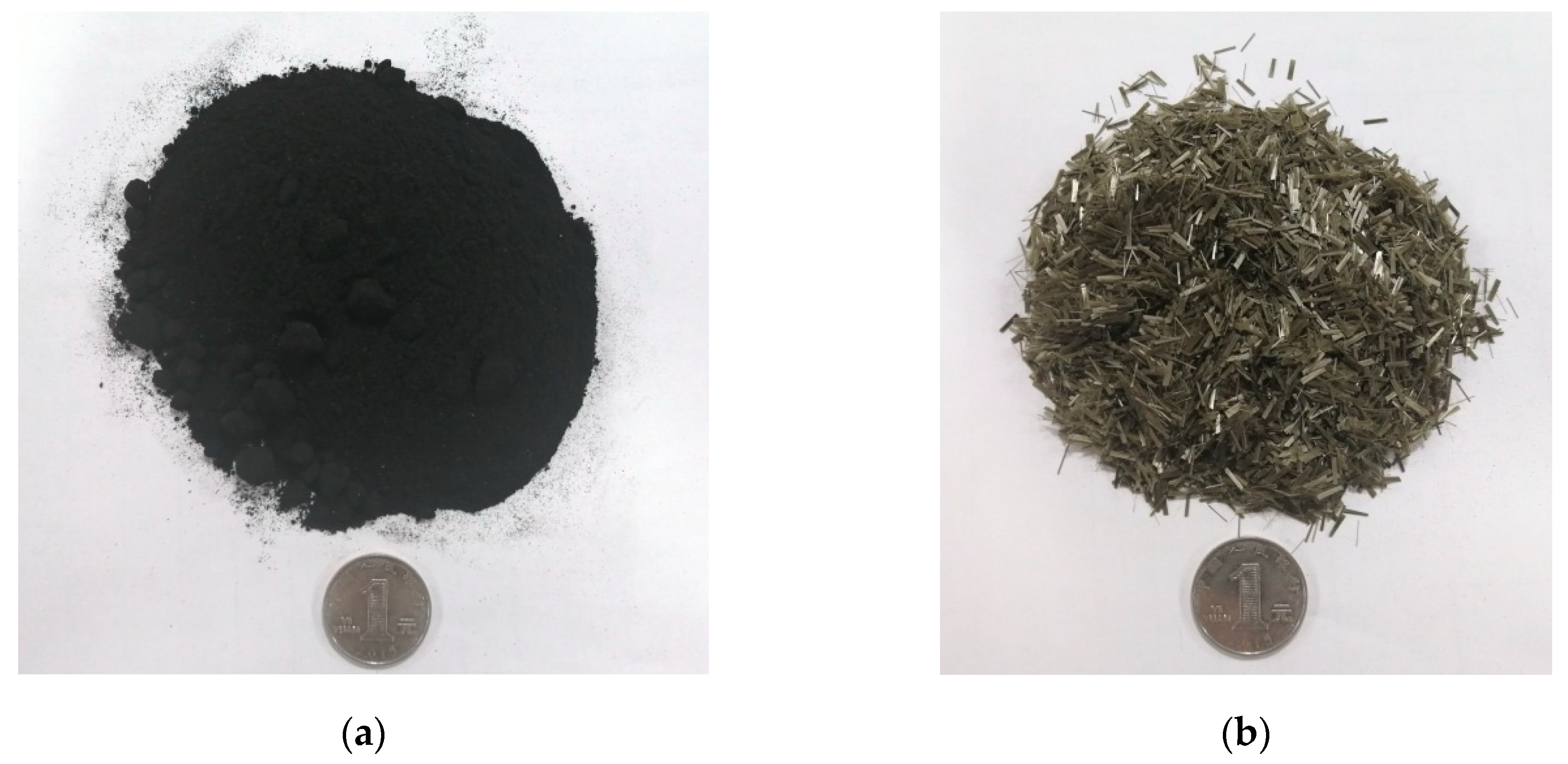
Figure 1.
Appearance of crumb rubber and basalt fiber: (a) crumb rubber; (b) basalt fiber.
Figure 1.
Appearance of crumb rubber and basalt fiber: (a) crumb rubber; (b) basalt fiber.
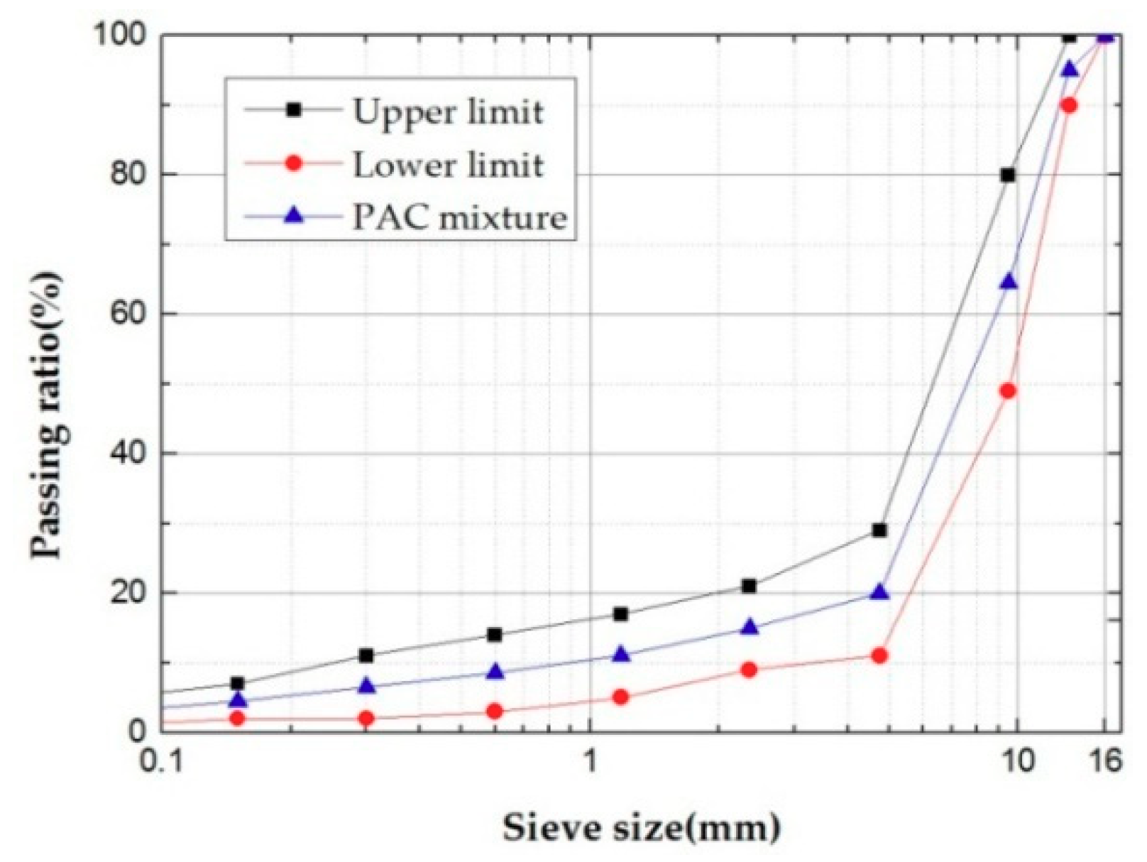
Figure 2.
Aggregate gradation of PAM.
Figure 2.
Aggregate gradation of PAM.
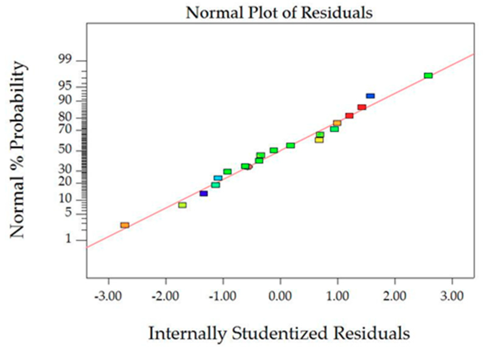
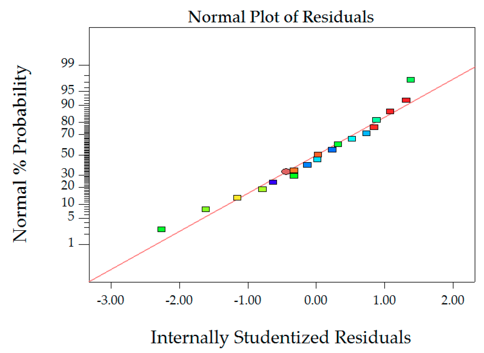
Figure 3.
Normal probability plot of VA.
Figure 3.
Normal probability plot of VA.
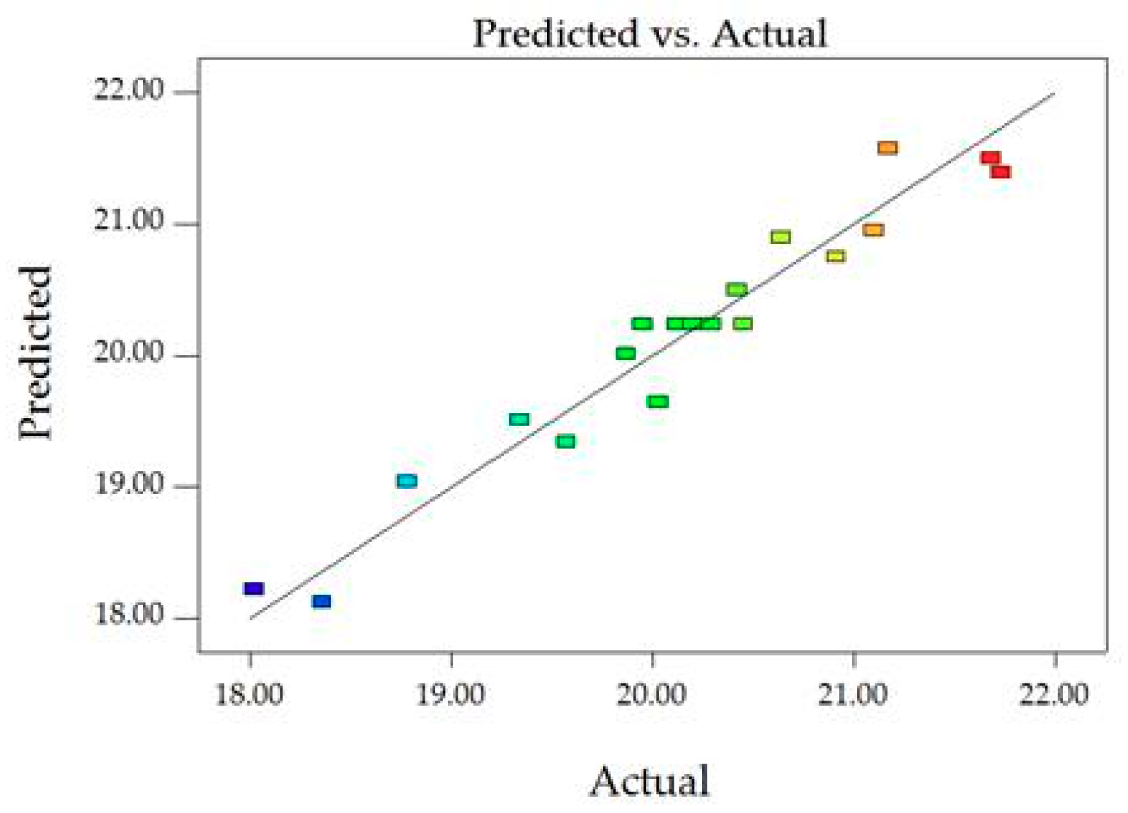
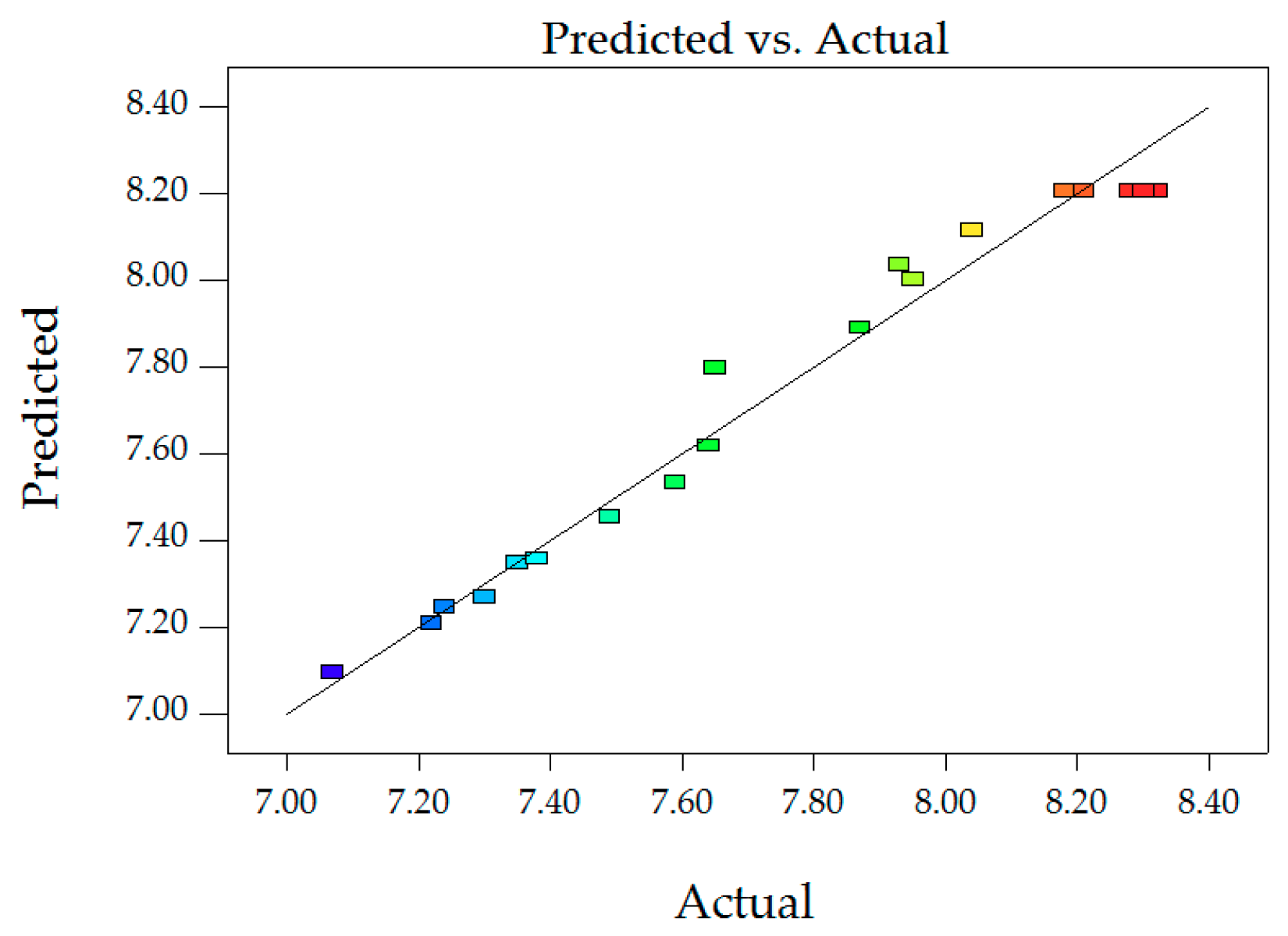
Figure 4.
Predictions and actual values of VA.
Figure 4.
Predictions and actual values of VA.
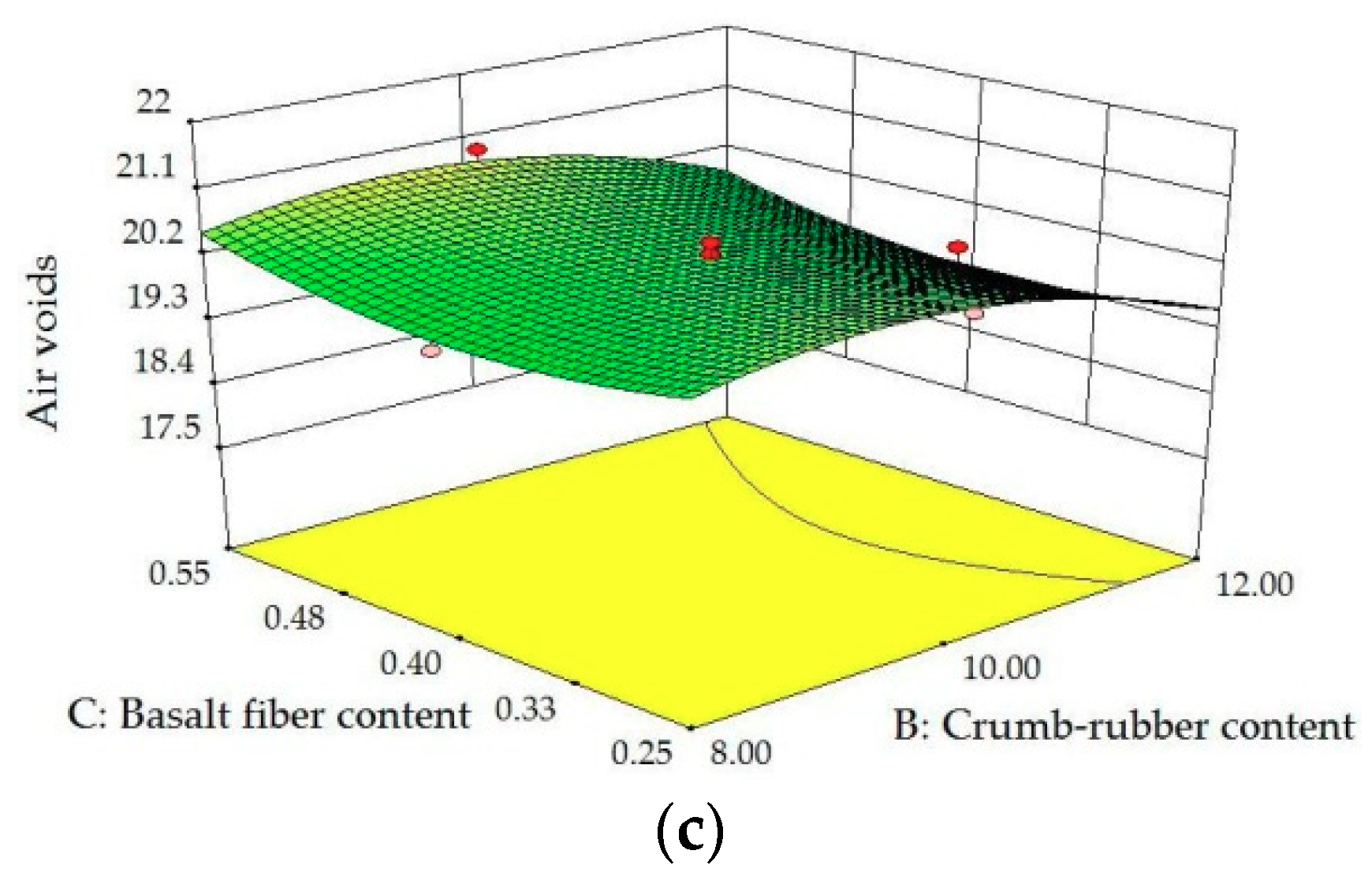
Figure 5.
3D surface plots between VA and factors: (a) Influence of A, B at C = 0.40; (b) influence of A, C at B = 10.0; (c) influence of B, C at A = 4.5.
Figure 5.
3D surface plots between VA and factors: (a) Influence of A, B at C = 0.40; (b) influence of A, C at B = 10.0; (c) influence of B, C at A = 4.5.
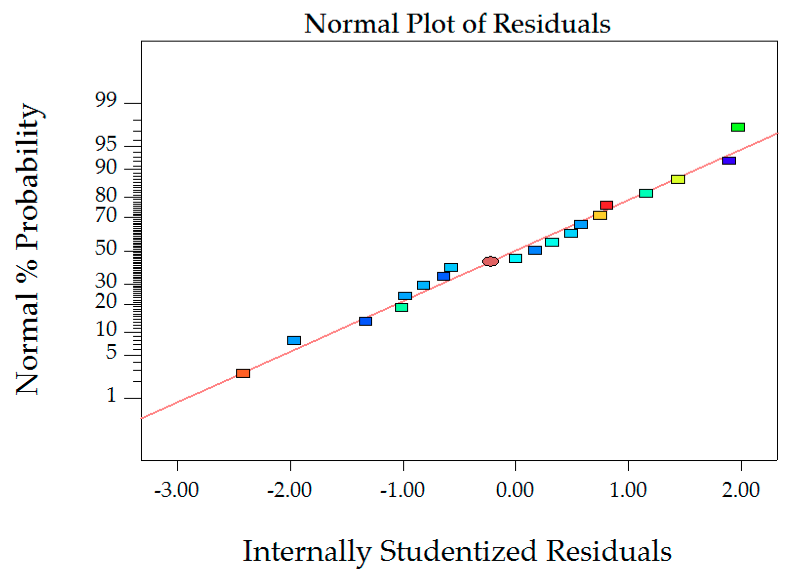
Figure 6.
Normal probability plot of MS.
Figure 6.
Normal probability plot of MS.
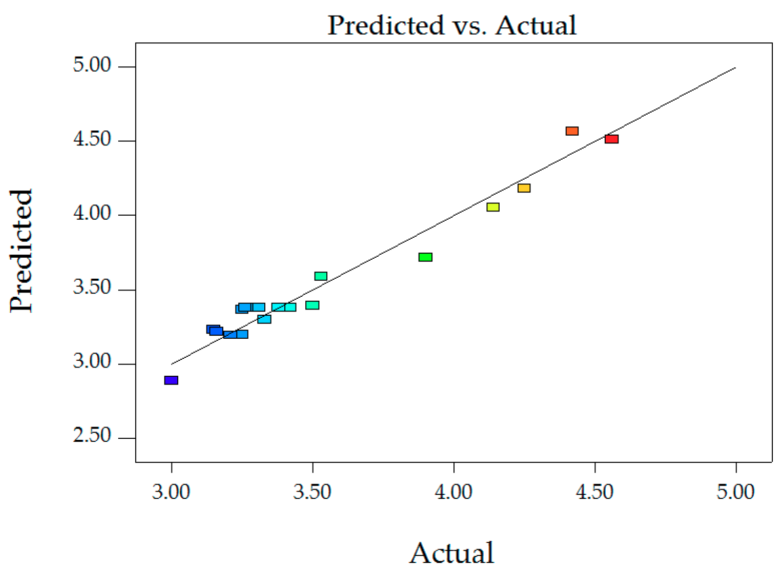
Figure 7.
Predictions and actual values of MS.
Figure 7.
Predictions and actual values of MS.
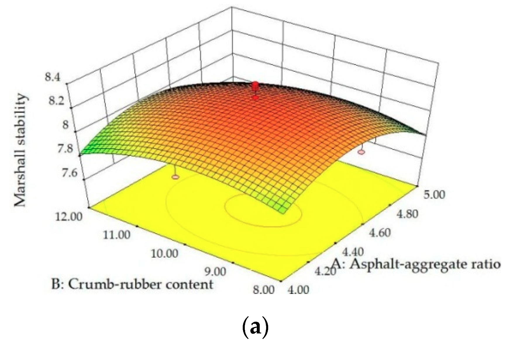
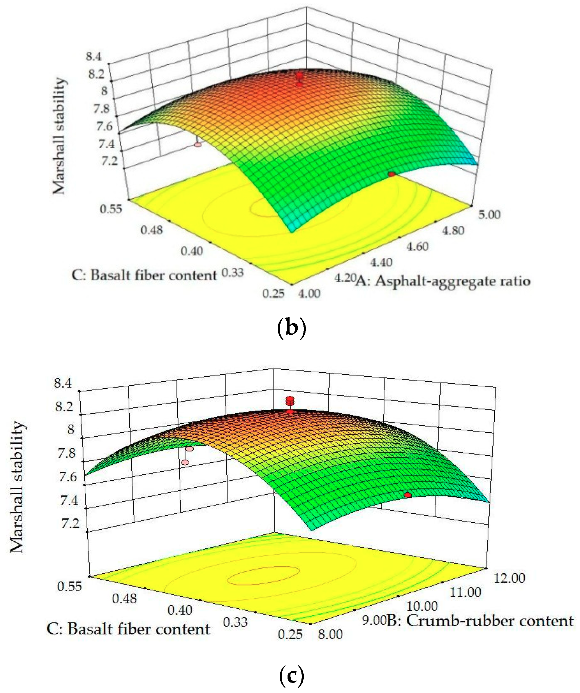
Figure 8.
3D surface plots between MS and factors: (a) Influence of A, B at C = 0.40; (b) influence of A, C at B = 10.0; (c) influence of B, C at A = 4.5.
Figure 8.
3D surface plots between MS and factors: (a) Influence of A, B at C = 0.40; (b) influence of A, C at B = 10.0; (c) influence of B, C at A = 4.5.
Figure 9.
Normal probability plot of FV.
Figure 9.
Normal probability plot of FV.
Figure 10.
Predictions and actual values FV.
Figure 10.
Predictions and actual values FV.
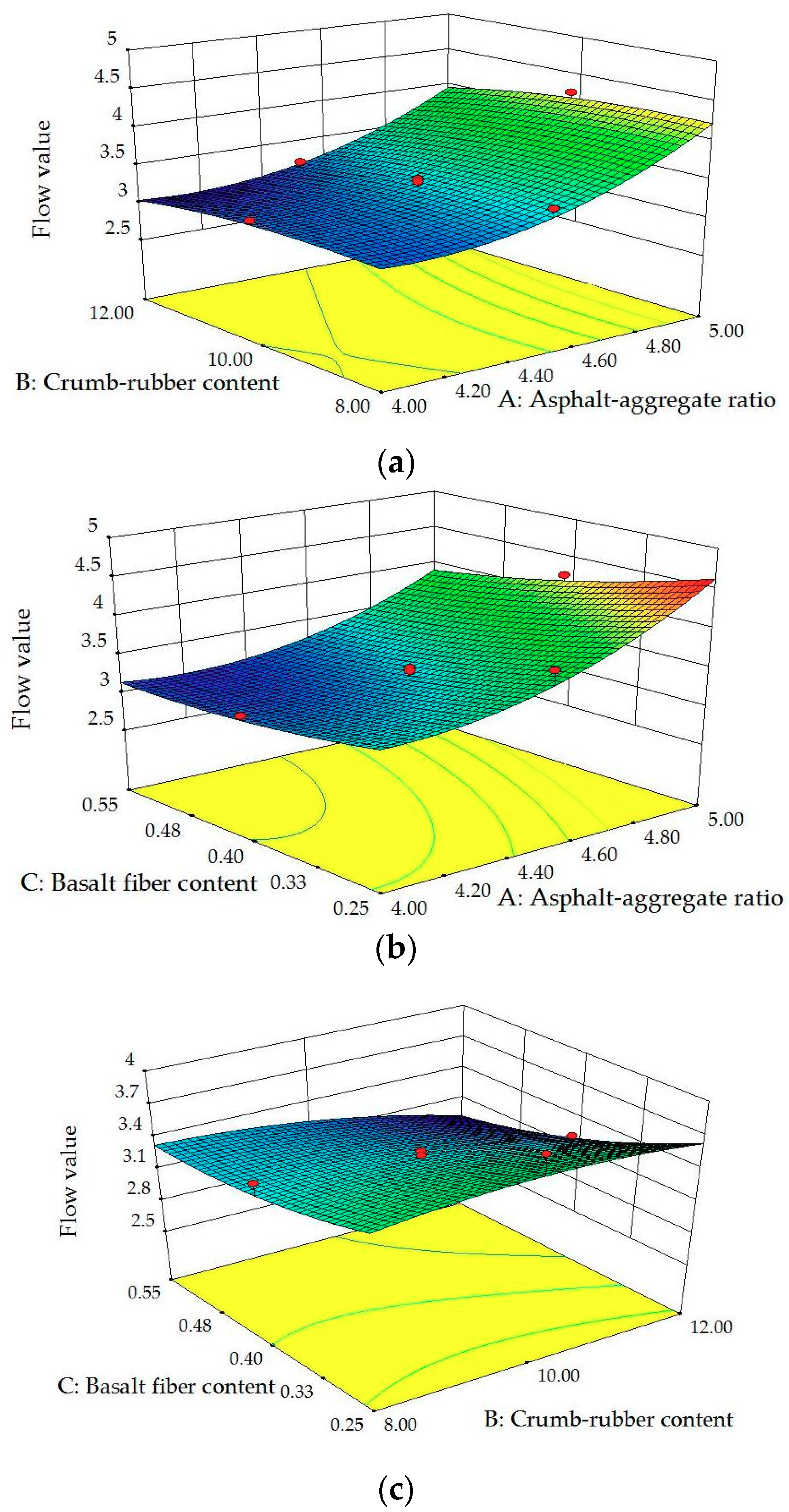
Figure 11.
3D surface plots between FV and factors: (a) Influence of A, B at C = 0.40; (b) influence of A, C at B = 10.0; (c) influence of B, C at A = 4.5.
Figure 11.
3D surface plots between FV and factors: (a) Influence of A, B at C = 0.40; (b) influence of A, C at B = 10.0; (c) influence of B, C at A = 4.5.
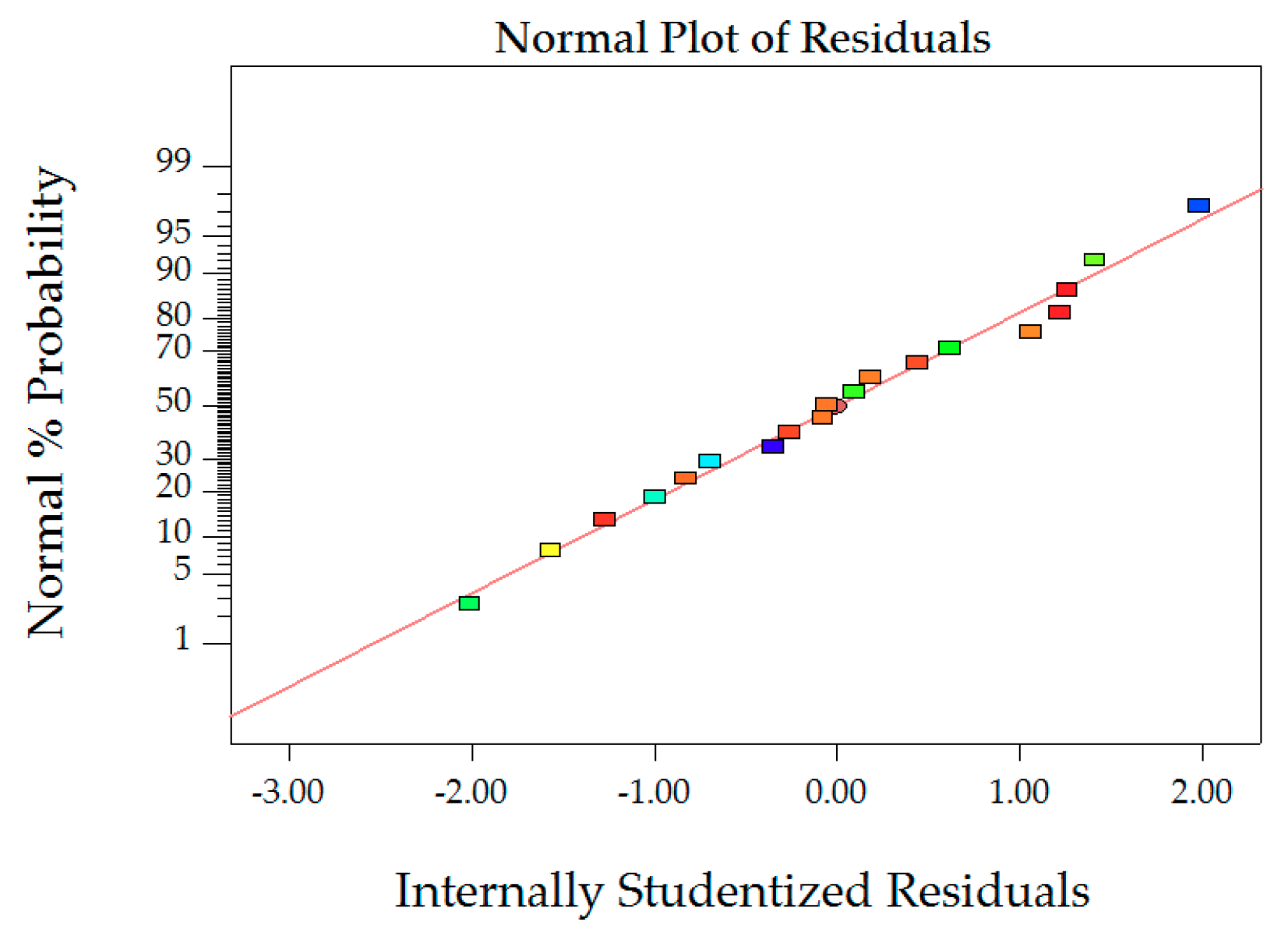
Figure 12.
Normal probability plot of MQ.
Figure 12.
Normal probability plot of MQ.
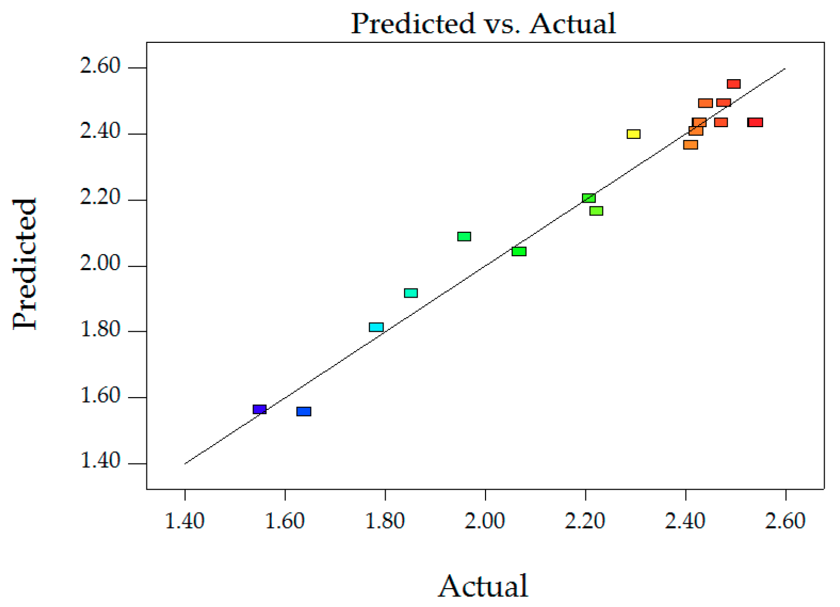
Figure 13.
Predictions and actual values of MQ.
Figure 13.
Predictions and actual values of MQ.
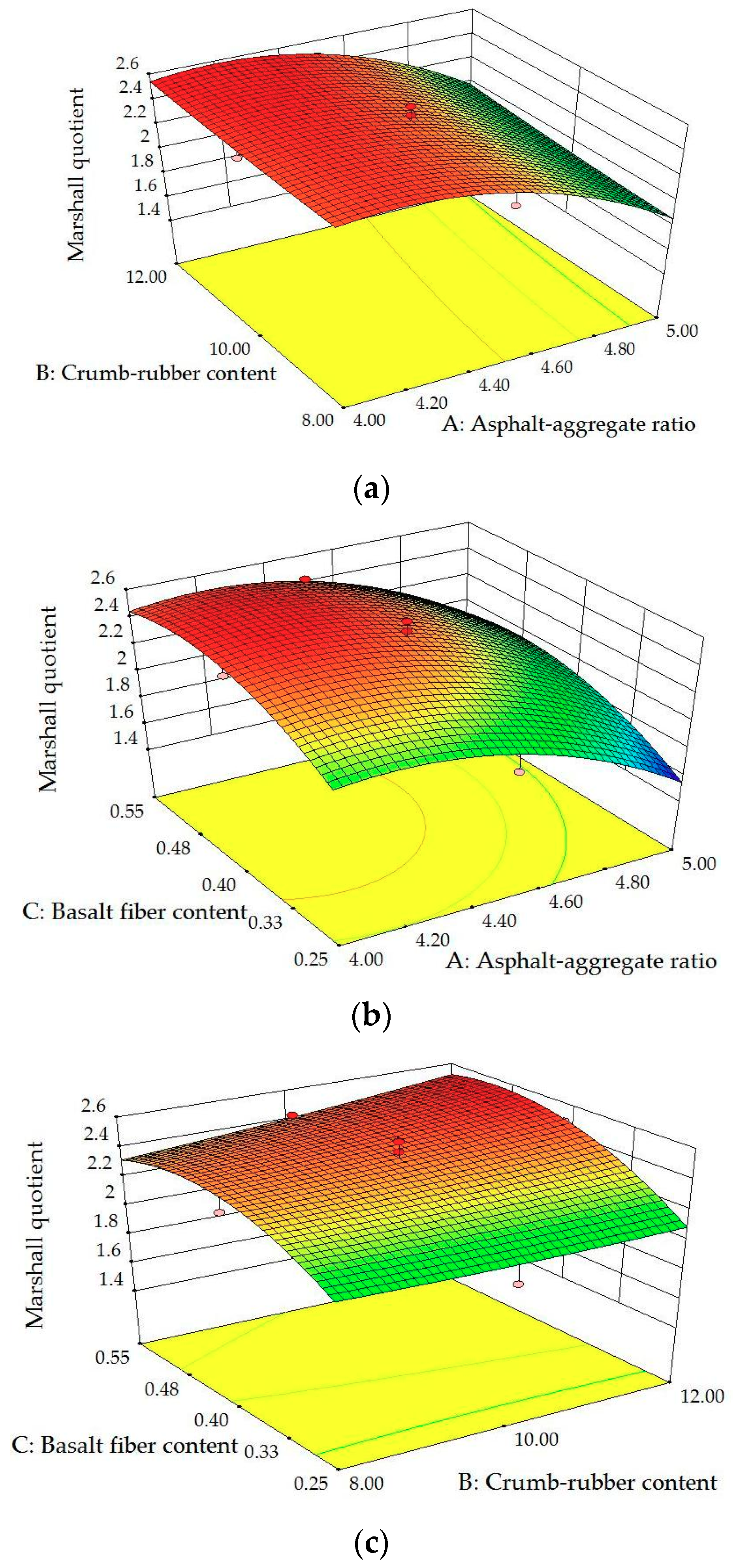
Figure 14.
3D surface plots between MQ and factors: (a) Influence of A, B at C = 0.40; (b) influence of A, C at B = 10.0; (c) influence of B, C at A = 4.5.
Figure 14.
3D surface plots between MQ and factors: (a) Influence of A, B at C = 0.40; (b) influence of A, C at B = 10.0; (c) influence of B, C at A = 4.5.
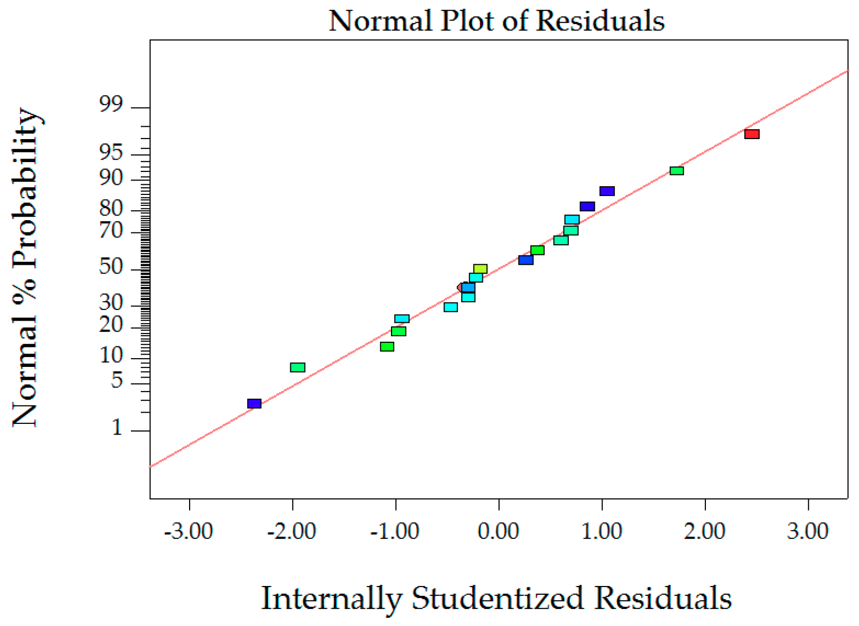
Figure 15.
Normal probability plot of CPL.
Figure 15.
Normal probability plot of CPL.
Figure 16.
Predictions and actual values CPL.
Figure 16.
Predictions and actual values CPL.
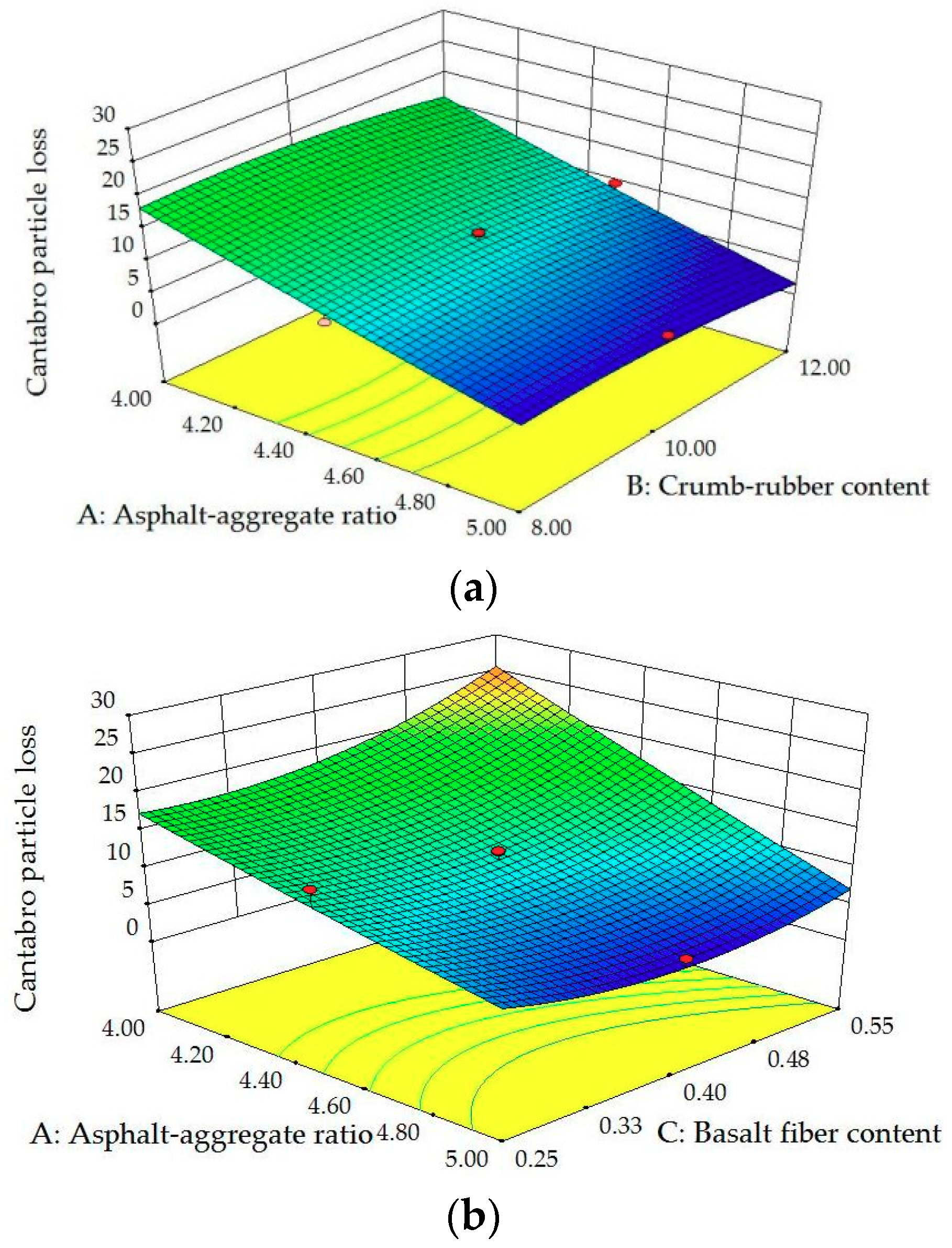
Figure 17.
3D surface plots between CPL and factors: (a) Influence of A, B at C = 0.40; (b) influence of A, C at B = 10.0; (c) influence of B, C at A = 4.5.
Figure 17.
3D surface plots between CPL and factors: (a) Influence of A, B at C = 0.40; (b) influence of A, C at B = 10.0; (c) influence of B, C at A = 4.5.
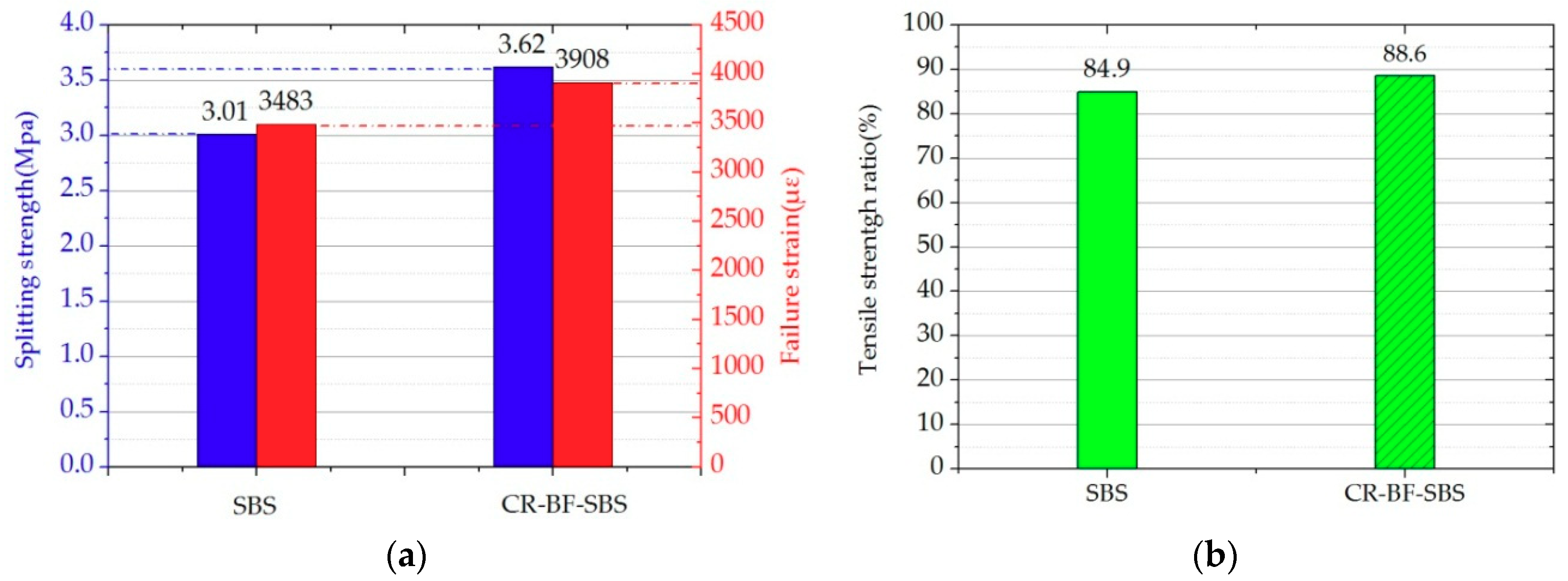
Figure 18.
Pavement performance test results: (a) Low-temperature cracking resistance; (b) moisture stability.
Figure 18.
Pavement performance test results: (a) Low-temperature cracking resistance; (b) moisture stability.
Table 1.
Properties of SBS-modified bitumen.
Table 1.
Properties of SBS-modified bitumen.
| Properties | Results | Chinese Standard |
|---|
| Penetration (25 °C, 0.1 mm) | 65.2 | 60–80 |
| Softening point (°C) | 64.2 | ≥55 |
| Ductility (5 °C, cm) | 34.5 | ≥30 |
| Flash point (°C) | 264 | ≥230 |
| Elastic recovery (25 °C, %) | 91.7 | ≥65 |
Table 2.
Properties of aggregates and filler.
Table 2.
Properties of aggregates and filler.
| Index | Apparent Specific Density (g/cm3) | Los Angeles Abrasion (%) | Crushed Stone Value (%) |
|---|
| Coarse aggregate | 3.527 | 12.9 | 13.9 |
| Fine aggregate | 3.389 | − | − |
| Filler | 2.722 | − | − |
Table 3.
Physical properties of crumb rubber.
Table 3.
Physical properties of crumb rubber.
| Properties | Results | Technical Criterion |
|---|
| Apparent density (g/cm3) | 1.18 | 1.1–1.3 |
| Metal content (%) | 0.038 | <0.05 |
| Moisture content (%) | 0.32 | <1 |
| Fiber content (%) | 0.43 | <1 |
| Ash content (%) | 4.5 | ≤8 |
Table 4.
Physical properties of basalt fiber.
Table 4.
Physical properties of basalt fiber.
| Index | Diameter | Length | Specific Gravity | Tensile Strength |
|---|
| Units | μm | mm | g/cm3 | MPa |
| Value | 13 | 6 | 2.63 | 2320 |
Table 5.
Experimental results of 19 groups.
Table 5.
Experimental results of 19 groups.
| Test Serial Number | Independent Variables | Responses |
|---|
| A | B | C | VA | MS | FV | MQ | CPL |
|---|
| (%) | (%) | (%) | (%) | (kN) | (mm) | (kN/mm) | (%) |
|---|
| 1 | 4.5 | 10 | 0.25 | 20.42 | 7.64 | 3.90 | 1.959 | 14.42 |
| 2 | 4 | 8 | 0.25 | 20.64 | 7.35 | 3.33 | 2.207 | 15.02 |
| 3 | 4.5 | 8 | 0.4 | 19.87 | 8.04 | 3.50 | 2.297 | 9.85 |
| 4 | 4.5 | 10 | 0.55 | 20.91 | 7.65 | 3.16 | 2.421 | 13.59 |
| 5 | 4 | 8 | 0.55 | 21.68 | 7.59 | 3.15 | 2.410 | 28.97 |
| 6 | 5 | 12 | 0.55 | 18.36 | 7.30 | 3.53 | 2.068 | 4.03 |
| 7 | 5 | 12 | 0.25 | 18.02 | 7.07 | 4.56 | 1.550 | 4.35 |
| 8 | 4.5 | 10 | 0.4 | 20.12 | 8.28 | 3.26 | 2.540 | 12.18 |
| 9 | 4.5 | 10 | 0.4 | 20.20 | 8.21 | 3.38 | 2.429 | 10.65 |
| 10 | 4 | 12 | 0.25 | 21.10 | 7.22 | 3.25 | 2.222 | 16.99 |
| 11 | 5 | 8 | 0.55 | 19.34 | 7.38 | 4.14 | 1.783 | 8.27 |
| 12 | 5 | 10 | 0.4 | 18.78 | 7.87 | 4.25 | 1.852 | 5.29 |
| 13 | 4.5 | 12 | 0.4 | 19.57 | 7.95 | 3.21 | 2.477 | 9.74 |
| 14 | 4.5 | 10 | 0.4 | 20.29 | 8.18 | 3.31 | 2.471 | 10.36 |
| 15 | 4.5 | 10 | 0.4 | 20.45 | 8.30 | 3.42 | 2.427 | 10.78 |
| 16 | 5 | 8 | 0.25 | 20.03 | 7.24 | 4.42 | 1.638 | 6.07 |
| 17 | 4 | 10 | 0.4 | 21.73 | 7.93 | 3.25 | 2.440 | 17.14 |
| 18 | 4.5 | 10 | 0.4 | 19.95 | 8.32 | 3.28 | 2.537 | 12.35 |
| 19 | 4 | 12 | 0.55 | 21.17 | 7.49 | 3.00 | 2.497 | 21.78 |
Table 6.
The ANOVA results of the VA model.
Table 6.
The ANOVA results of the VA model.
| | Quadratic Sum | DF | Mean Square | R2 | Adj. R2 | F Value | p Value | Significant |
|---|
| Model | 17.53 | 9 | 1.95 | 0.9463 | 0.8926 | 17.63 | 0.0001 | √ |
| Residual error | 0.99 | 9 | 0.11 | | | | | |
| Lack of fit | 0.86 | 5 | 0.17 | | | 4.9 | 0.0743 | × |
| Pure error | 0.14 | 4 | 0.035 | | | | | |
| Sum | 18.52 | 18 | | | | | | |
Table 7.
The ANOVA results of independent variables in VA model.
Table 7.
The ANOVA results of independent variables in VA model.
| Factors | Sum of Squares | DF | Mean Square | F Value | p Value | Significant |
|---|
| A | 13.90 | 1 | 13.9 | 125.78 | <0.0001 | **** |
| B | 1.12 | 1 | 1.12 | 10.09 | 0.0112 | * |
| C | 0.16 | 1 | 0.16 | 1.41 | 0.2648 | − |
| AB | 1.08 | 1 | 1.08 | 9.78 | 0.0122 | * |
| AC | 0.27 | 1 | 0.27 | 2.41 | 0.1549 | − |
| BC | 0.00045 | 1 | 0.00045 | 0.004 | 0.9505 | − |
| A2 | 0.00096 | 1 | 0.00096 | 0.008 | 0.9275 | − |
| B2 | 0.84 | 1 | 0.84 | 7.58 | 0.0223 | * |
| C2 | 0.42 | 1 | 0.42 | 3.78 | 0.0836 | − |
Table 8.
The ANOVA results of the MS model.
Table 8.
The ANOVA results of the MS model.
| | Quadratic Sum | DF | Mean Square | R2 | Adj. R2 | F Value | p Value | Significant |
|---|
| Model | 3.01 | 9 | 0.33 | 0.9754 | 0.9509 | 39.69 | <0.0001 | √ |
| Residual error | 0.076 | 9 | 0.0084 | | | | | |
| Lack of fit | 0.061 | 5 | 0.012 | | | 3.40 | 0.1298 | × |
| Pure error | 0.014 | 4 | 0.0036 | | | | | |
| Sum | 3.09 | 18 | | | | | | |
Table 9.
The ANOVA results of independent variables in MS model.
Table 9.
The ANOVA results of independent variables in MS model.
| Factors | Sum of Squares | DF | Mean Square | F Value | p Value | Significant |
|---|
| A | 0.052 | 1 | 0.052 | 6.14 | 0.0351 | * |
| B | 0.032 | 1 | 0.032 | 3.85 | 0.0814 | − |
| C | 0.079 | 1 | 0.079 | 9.39 | 0.0135 | * |
| AB | 0.00005 | 1 | 0.00005 | 0.0059 | 0.9403 | − |
| AC | 0.0024 | 1 | 0.0024 | 0.29 | 0.6031 | − |
| BC | 0.0018 | 1 | 0.0018 | 0.21 | 0.6552 | − |
| A2 | 0.16 | 1 | 0.16 | 19.34 | 0.0017 | ** |
| B2 | 0.061 | 1 | 0.061 | 7.23 | 0.0248 | * |
| C2 | 0.68 | 1 | 0.68 | 80.76 | <0.0001 | **** |
Table 10.
The ANOVA results of FV model.
Table 10.
The ANOVA results of FV model.
| | Quadratic Sum | DF | Mean Square | R2 | Adj. R2 | F Value | p Value | Significant |
|---|
| Model | 3.80 | 9 | 0.42 | 0.9604 | 0.9209 | 24.28 | <0.0001 | √ |
| Residual error | 0.16 | 9 | 0.017 | | | | | |
| Lack of fit | 0.14 | 5 | 0.028 | | | 6.01 | 0.0535 | × |
| Pure error | 0.018 | 4 | 0.0046 | | | | | |
| Sum | 3.96 | 18 | | | | | | |
Table 11.
The ANOVA results of independent variables in the FV model.
Table 11.
The ANOVA results of independent variables in the FV model.
| Factors | Sum of Squares | DF | Mean Square | F Value | p Value | Significant |
|---|
| A | 2.42 | 1 | 2.42 | 139.12 | <0.0001 | **** |
| B | 0.098 | 1 | 0.098 | 5.63 | 0.0417 | * |
| C | 0.62 | 1 | 0.62 | 35.35 | 0.0002 | *** |
| AB | 0.0072 | 1 | 0.0072 | 0.41 | 0.5361 | − |
| AC | 0.097 | 1 | 0.097 | 5.56 | 0.0427 | * |
| BC | 0.084 | 1 | 0.084 | 4.83 | 0.0555 | − |
| A2 | 0.26 | 1 | 0.26 | 14.87 | 0.0039 | ** |
| B2 | 0.021 | 1 | 0.021 | 1.20 | 0.3025 | − |
| C2 | 0.021 | 1 | 0.021 | 1.21 | 0.3001 | − |
Table 12.
The ANOVA results of MQ model.
Table 12.
The ANOVA results of MQ model.
| | Quadratic Sum | DF | Mean Square | R2 | Adj. R2 | F Value | p Value | Significant |
|---|
| Model | 1.76 | 9 | 0.20 | 0.9594 | 0.9189 | 23.66 | <0.0001 | √ |
| Residual error | 0.074 | 9 | 0.0082 | | | | | |
| Lack of fit | 0.062 | 5 | 0.012 | | | 4.02 | 0.1013 | × |
| Pure error | 0.012 | 4 | 0.003 | | | | | |
| Sum | 1.83 | 18 | | | | | | |
Table 13.
The ANOVA results of the independent variables in the MQ model.
Table 13.
The ANOVA results of the independent variables in the MQ model.
| Factors | Sum of Squares | DF | Mean Square | F Value | p Value | Significant |
|---|
| A | 0.83 | 1 | 0.83 | 100.86 | <0.0001 | **** |
| B | 0.023 | 1 | 0.023 | 2.78 | 0.1298 | − |
| C | 0.26 | 1 | 0.26 | 31.14 | 0.0003 | *** |
| AB | 0.0011 | 1 | 0.0011 | 0.14 | 0.7201 | − |
| AC | 0.0042 | 1 | 0.0042 | 0.52 | 0.4898 | − |
| BC | 0.025 | 1 | 0.025 | 3.00 | 0.1173 | − |
| A2 | 0.14 | 1 | 0.14 | 17.34 | 0.0024 | ** |
| B2 | 0.0004 | 1 | 0.0004 | 0.049 | 0.8300 | − |
| C2 | 0.093 | 1 | 0.093 | 11.31 | 0.0083 | ** |
Table 14.
The ANOVA results of the CPL model.
Table 14.
The ANOVA results of the CPL model.
| | Quadratic Sum | DF | Mean Square | R2 | Adj. R2 | F Value | p Value | Significant |
|---|
| Model | 653.35 | 9 | 72.59 | 0.9556 | 0.9112 | 21.52 | <0.0001 | √ |
| Residual error | 30.37 | 9 | 3.37 | | | | | |
| Lack of fit | 26.92 | 5 | 5.38 | | | 6.25 | 0.0501 | × |
| Pure error | 3.45 | 4 | 0.86 | | | | | |
| Sum | 683.71 | 18 | | | | | | |
Table 15.
The ANOVA results of the independent variables in the CPL model.
Table 15.
The ANOVA results of the independent variables in the CPL model.
| Factors | Sum of Squares | DF | Mean Square | F Value | p Value | Significant |
|---|
| A | 516.82 | 1 | 516.82 | 153.18 | <0.0001 | **** |
| B | 12.75 | 1 | 12.75 | 3.78 | 0.0838 | − |
| C | 39.16 | 1 | 39.16 | 11.61 | 0.0078 | ** |
| AB | 0.068 | 1 | 0.068 | 0.020 | 0.8899 | − |
| AC | 35.53 | 1 | 35.53 | 10.53 | 0.0101 | * |
| BC | 17.05 | 1 | 17.05 | 5.05 | 0.0512 | − |
| A2 | 0.12 | 1 | 0.12 | 0.036 | 0.8543 | − |
| B2 | 4.00 | 1 | 4.00 | 1.19 | 0.3045 | − |
| C2 | 24.59 | 1 | 24.59 | 7.29 | 0.0244 | * |
Table 16.
Target values of response variables.
Table 16.
Target values of response variables.
| Response | VA (Y1) | MS (Y2) | FV (Y3) | MQ (Y4) | CPL (Y5) |
|---|
| Units | % | kN | mm | kN/mm | % |
| Target value | 18–22 | Maximize | 2–4 | Maximize | Minimize |
Table 17.
Optimal preparation parameters and prediction vs. experiment.
Table 17.
Optimal preparation parameters and prediction vs. experiment.
| Response | A (%) | B (%) | C (%) | VA (%) | MS (kN) | FV (mm) | MQ (kN/mm) | CPL (%) |
|---|
| Prediction | 4.51 | 11.21 | 0.42 | 19.82 | 8.12 | 3.26 | 2.48 | 10.03 |
| Experiment | 4.51 | 11.21 | 0.42 | 20.16 | 7.92 | 3.34 | 2.37 | 10.38 |
| Chinese Standard | − | − | − | 18–25 | ≥5 | 2–4 | − | <15 |
| Relative error (%) | − | − | − | 1.70 | −2.46 | −2.45 | −4.38 | 3.49 |


