Unveiling Key Drivers of Indirect Carbon Emissions of Chinese Older Households


Abstract
1. Introduction
2. Materials and Methods
2.1. Calculation of Indirect Carbon Emissions
2.2. Unconditional Quantile Regression
2.3. Data Sources and Processing
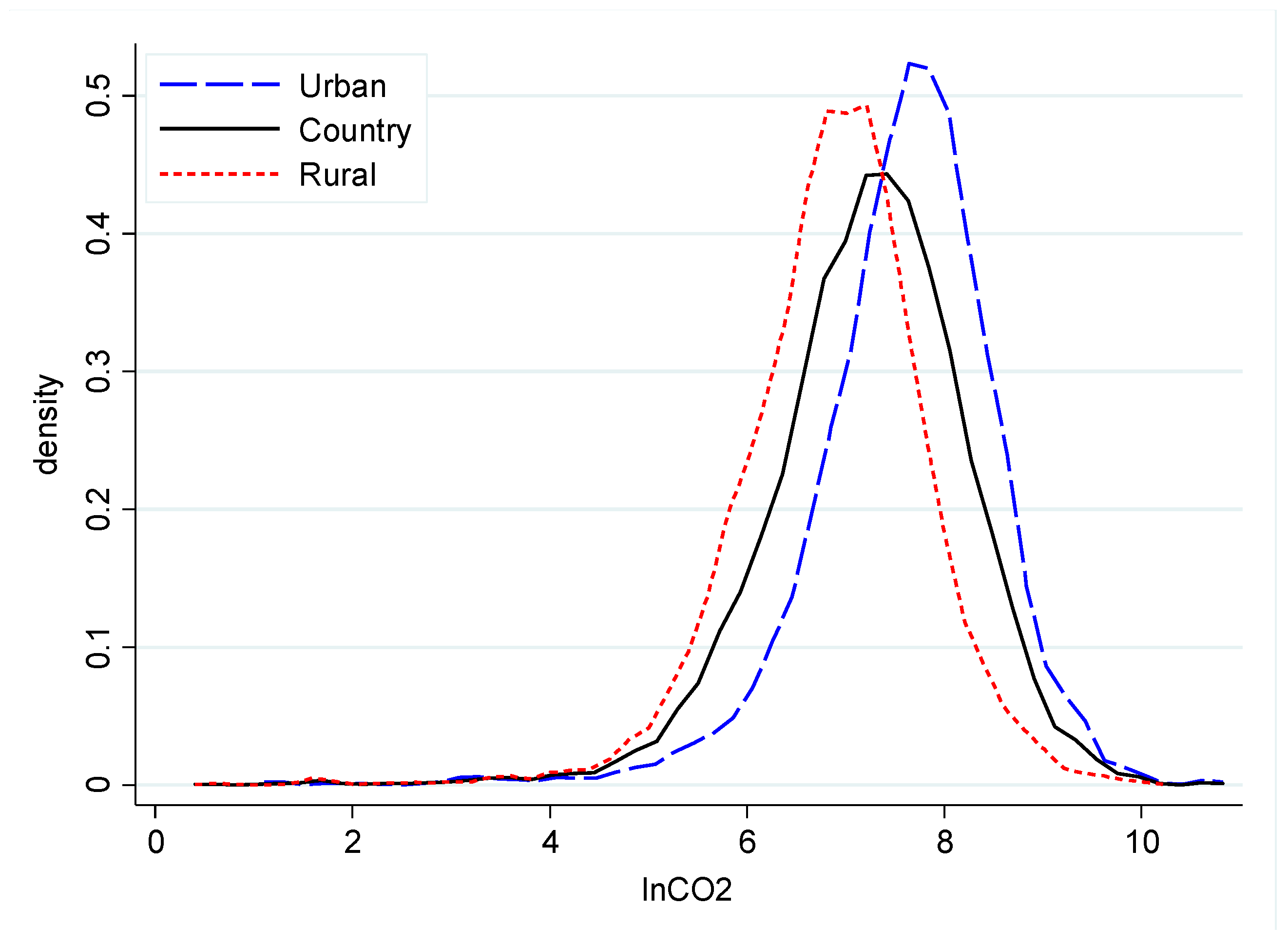
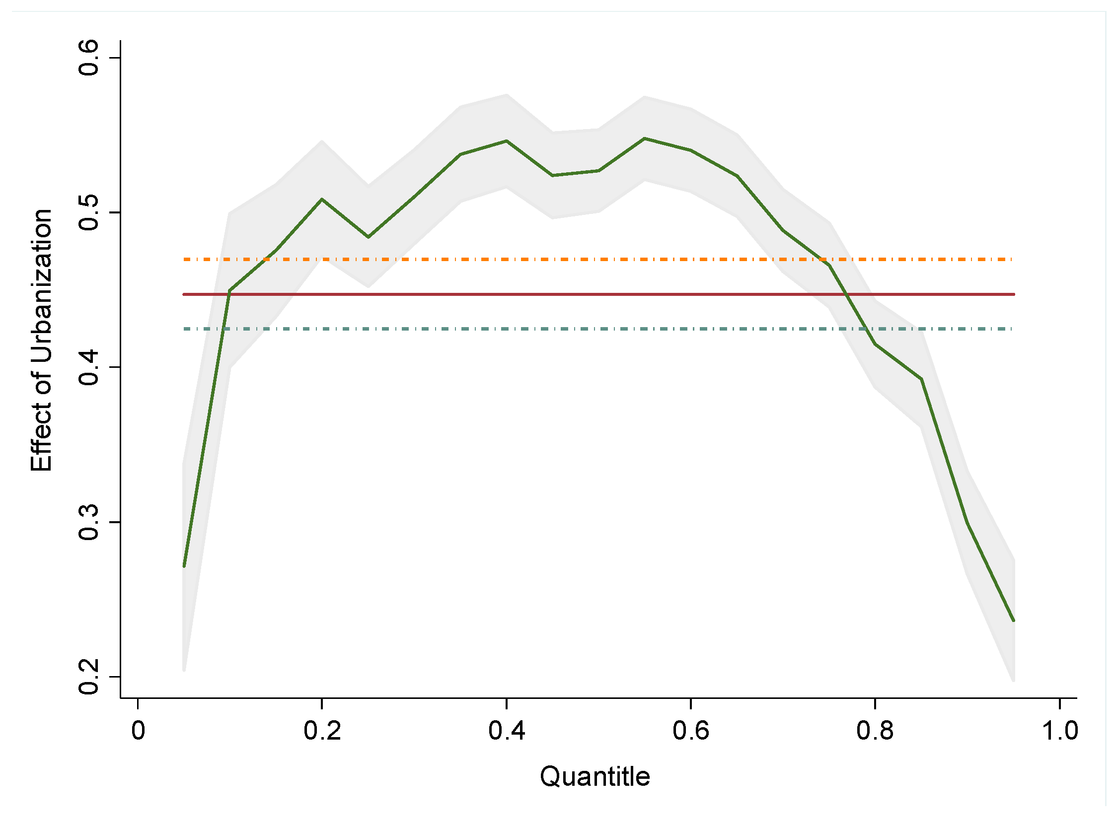
3. Results
3.1. Effects of Urbanization on Indirect Carbon Emissions
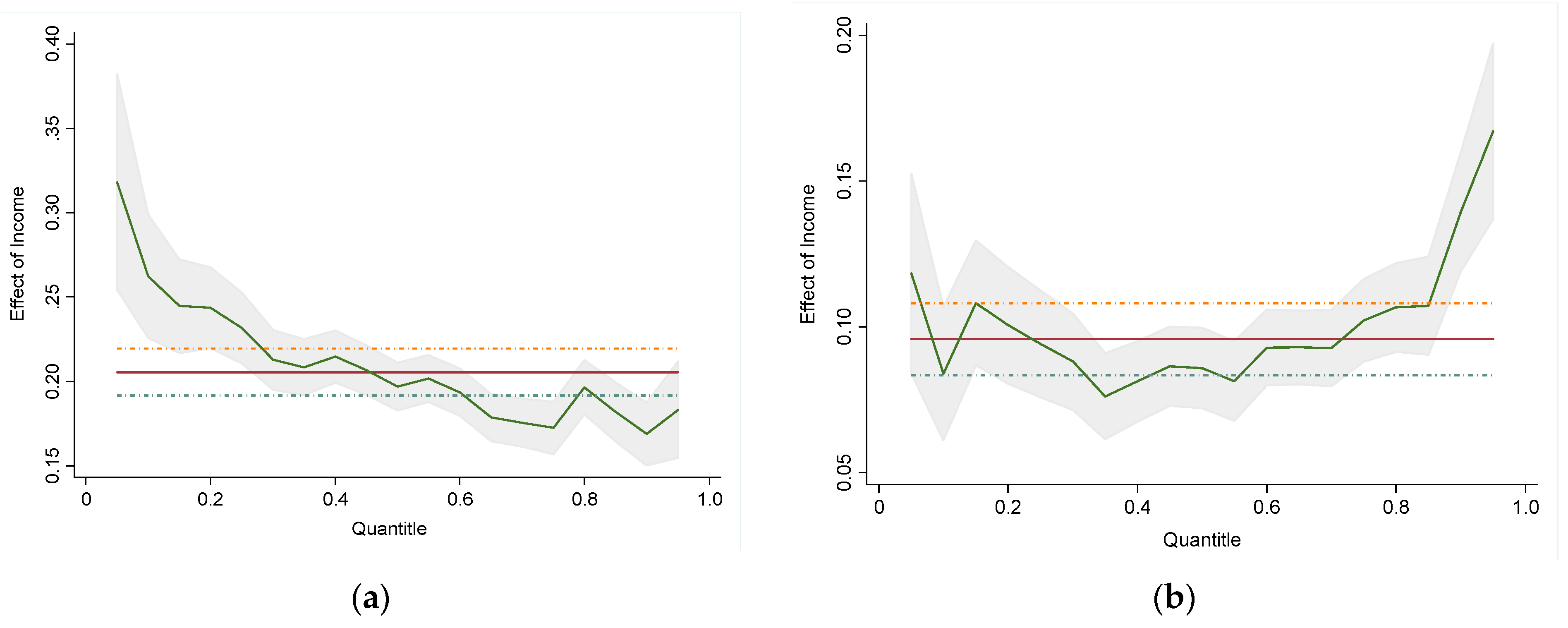
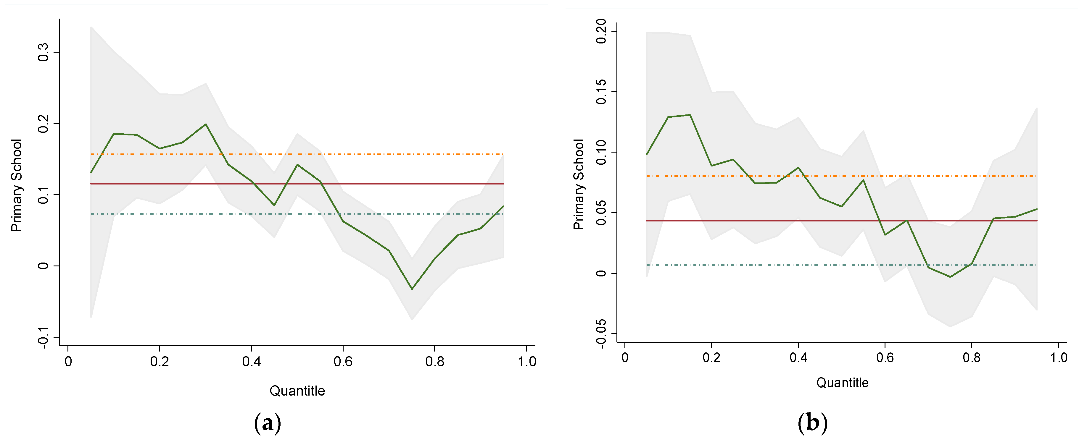
3.2. Determinants of Per Capita Indirect Carbon Emissions in Urban China
3.3. Determinants of Per Capita Indirect CO2 Emissions in Rural China
3.4. Different Effects of Determinants between Urban and Rural Households
3.4.1. Income
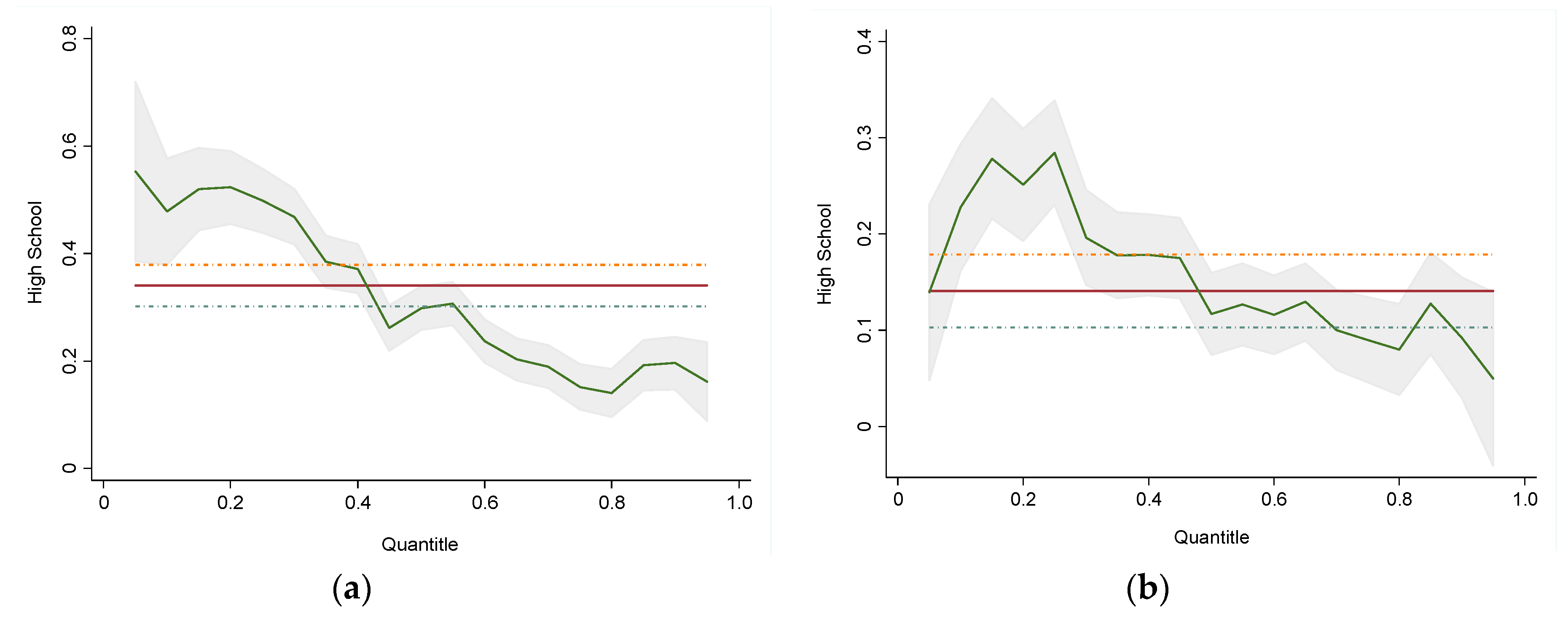
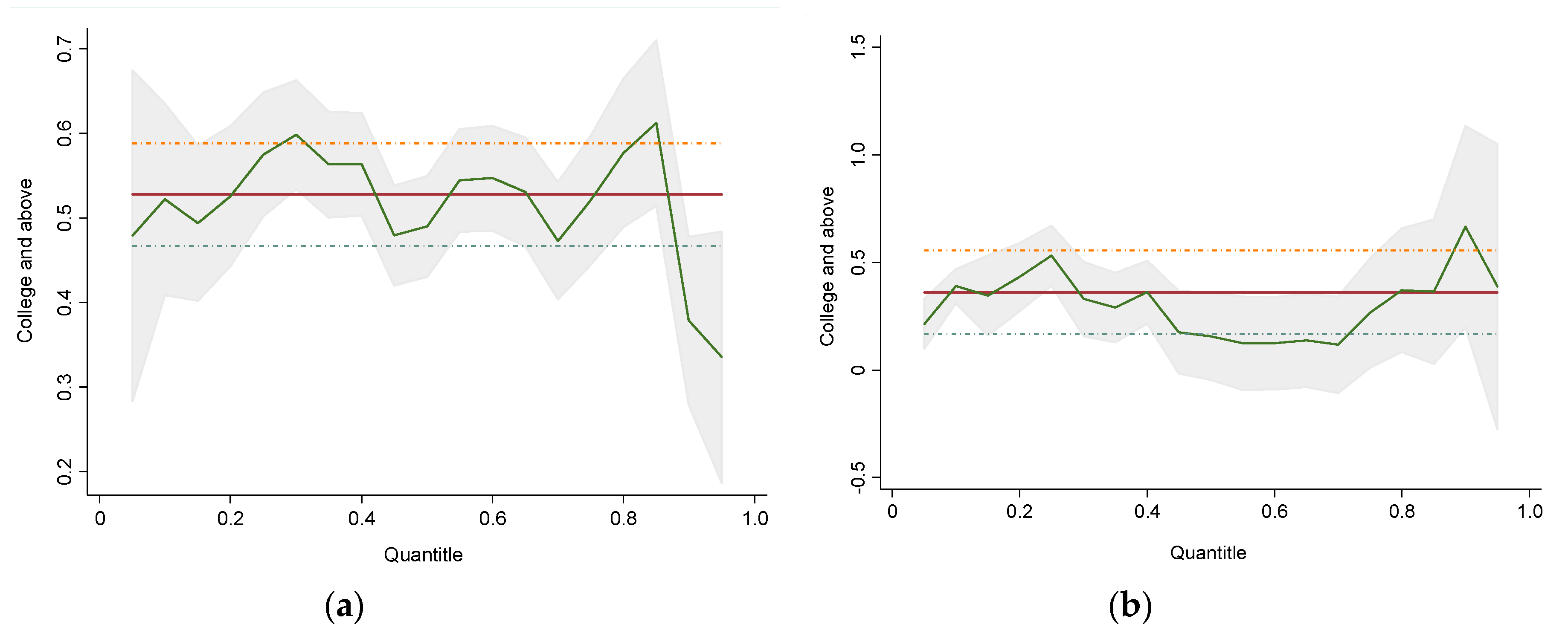
3.4.2. Education
3.4.3. Other Determinants
4. Discussion
- Due to data availability, when calculating the indirect carbon emissions, we use input-output tables and sectoral CO2 emissions data from WIOD in China for 2007 to quantify emissions for 2013. Therefore, we are making an assumption that the production technology, as well as the sectoral carbon intensities in 2013, is the same as that of 2007.
- We rely on China’s input-output table instead of the multi-regional input-output table to approximate emissions from imports, which means that the carbon intensities of the imported goods and services consumed by households are the same as that of goods and services produced in China. Further studies can be undertaken to measure household carbon emissions more completely by using a multi-regional input-output table.
- While input-output analysis has a certain advantage over a process-based life cycle assessment because it is more comprehensive, it is also much coarser, which makes the analysis less accurate and relevant [54]. As the hybrid life cycle assessment unites the precision of a process-based life cycle assessment with the comprehensiveness of input-output analysis [55], it will be very helpful to utilize the hybrid life cycle assessment in the future study.
- There are 35 sectors in China’s input-output table, but we only have 24 expenditure items of goods and services in CHARLS to complete the data match and quantify the indirect carbon emissions. It would be more helpful if we have detailed consumption expenditure items.
- Considering that the research results regarding the relationship between education and household carbon emissions in the literature are inconclusive, it is of critical importance to study the influencing mechanism of education on household carbon emissions in China in future research.
- This paper only focuses on indirect carbon emissions of households whose heads are more than 45 years old, and further comparative study between households with the heads less than 45 years old and more than 45 years old will be helpful to mitigation policies.
Author Contributions
Funding
Conflicts of Interest
References
- Zhang, Y.J.; Bian, X.J.; Tan, W. The linkages of sectoral carbon dioxide emission caused by household consumption in China: Evidence from the hypothetical extraction method. Empir. Econ. 2018, 54, 1743–1775. [Google Scholar] [CrossRef]
- Bin, S.; Dowlatabadi, H. Consumer lifestyle approach to US energy use and the related CO2 emissions. Energy Policy 2005, 33, 197–208. [Google Scholar] [CrossRef]
- Pachauri, S.; Spreng, D. Direct and indirect energy requirements of households in India. Energy Policy 2002, 30, 511–523. [Google Scholar] [CrossRef]
- Park, H.C.; Heo, E. The direct and indirect household energy requirements in the Republic of Korea from 1980 to 2000-An input-output analysis. Energy Policy 2007, 35, 2839–2851. [Google Scholar] [CrossRef]
- Nansai, K.; Kondo, Y.; Kagawa, S.; Suh, S.; Nakajima, K.; Inaba, R.; Tohno, S. Estimates of embodied global energy and air-emission intensities of japanese products for building a Japanese input-output life cycle assessment database with a global system boundary. Environ. Sci. Technol. 2012, 46, 9146–9154. [Google Scholar] [CrossRef] [PubMed]
- Hamamoto, M. Energy-saving behavior and marginal abatement cost for household CO2 emissions. Energy Policy 2013, 63, 809–813. [Google Scholar] [CrossRef]
- Markaki, M.; Belegri-Roboli, A.; Sarafidis, Y.; Mirasgedis, S. The carbon footprint of Greek households (1995–2012). Energy Policy 2017, 100, 206–215. [Google Scholar] [CrossRef]
- Liu, H.T.; Guo, J.E.; Qian, D.; Xi, Y.M. Comprehensive evaluation of household indirect energy consumption and impacts of alternative energy policies in China by input-output analysis. Energy Policy 2009, 37, 3194–3204. [Google Scholar] [CrossRef]
- Yang, Y.; Zhao, T.; Wang, Y.; Shi, Z. Research on impacts of population-related factors on carbon emissions in Beijing from 1984 to 2012. Environ. Impact Assess. Rev. 2015, 55, 45–53. [Google Scholar] [CrossRef]
- Zhang, C.; Tan, Z. The relationships between population factors and China’s carbon emissions: Does population aging matter? Renew. Sustain. Energy Rev. 2016, 65, 1018–1025. [Google Scholar] [CrossRef]
- Dalton, M.; O’Neill, B.; Prskawetz, A.; Jiang, L.; Pitkin, J. Population aging and future carbon emissions in the United States. Energy Econ. 2008, 30, 642–675. [Google Scholar] [CrossRef]
- Zhang, X.; Luo, L.; Skitmore, M. Household carbon emission research: An analytical review of measurement, influencing factors and mitigation prospects. J. Clean. Prod. 2015, 103, 873–883. [Google Scholar] [CrossRef]
- Yuan, B.; Ren, S.; Chen, X. The effects of urbanization, consumption ratio and consumption structure on residential indirect CO2 emissions in China: A regional comparative analysis. Appl. Energy 2015, 140, 94–106. [Google Scholar] [CrossRef]
- Ma, X.W.; Du, J.; Zhang, M.Y.; Ye, Y. Indirect carbon emissions from household consumption between China and the USA: Based on an input–output model. Nat. Hazards 2016, 84, 399–410. [Google Scholar] [CrossRef]
- Shen, W.; Cao, L.; Li, Q.; Zhang, W.; Wang, G.; Li, C. Quantifying CO2 emissions from China’s cement industry. Renew. Sustain. Energy Rev. 2015, 50, 1004–1012. [Google Scholar] [CrossRef]
- Heinonen, J.; Junnila, S. A carbon consumption comparison of rural and urban lifestyles. Sustainability 2011, 3, 1234–1249. [Google Scholar] [CrossRef]
- Feng, Z.H.; Zou, L.L.; Wei, Y.M. The impact of household consumption on energy use and CO2 emissions in China. Energy 2011, 36, 656–670. [Google Scholar] [CrossRef]
- Xu, X.; Han, L.; Lv, X. Household carbon inequality in urban China, its sources and determinants. Ecol. Econ. 2016, 128, 77–86. [Google Scholar] [CrossRef]
- Golley, J.; Meng, X. Income inequality and carbon dioxide emissions: The case of Chinese urban households. Energy Econ. 2012, 34, 1864–1872. [Google Scholar] [CrossRef]
- Zhang, L.X.; Wang, C.B.; Bahaj, A.S. Carbon emissions by rural energy in China. Renew. Energy 2014, 66, 641–649. [Google Scholar] [CrossRef]
- Wang, Z.; Liu, W.; Yin, J. Driving forces of indirect carbon emissions from household consumption in China: An input–output decomposition analysis. Nat. Hazards 2015, 75, 257–272. [Google Scholar] [CrossRef]
- López, L.A.; Arce, G.; Morenate, M.; Monsalve, F. Assessing the Inequality of Spanish Households through the Carbon Footprint: The 21st Century Great Recession Effect. J. Ind. Ecol. 2016, 20, 571–581. [Google Scholar] [CrossRef]
- Wiedenhofer, D.; Guan, D.; Liu, Z.; Meng, J.; Zhang, N.; Wei, Y.M. Unequal household carbon footprints in China. Nat. Clim. Chang. 2017, 7, 75–80. [Google Scholar] [CrossRef]
- Sommer, M.; Kratena, K. The Carbon Footprint of European Households and Income Distribution. Ecol. Econ. 2017, 136, 62–72. [Google Scholar] [CrossRef]
- Brand, C.; Goodman, A.; Rutter, H.; Song, Y.; Ogilvie, D. Associations of individual, household and environmental characteristics with carbon dioxide emissions from motorised passenger travel. Appl. Energy 2013, 104, 158–169. [Google Scholar] [CrossRef]
- Sun, C.; Ouyang, X.; Cai, H.; Luo, Z.; Li, A. Household pathway selection of energy consumption during urbanization process in China. Energy Convers. Manag. 2014, 84, 295–304. [Google Scholar] [CrossRef]
- Han, L.; Xu, X.; Han, L. Applying quantile regression and Shapley decomposition to analyzing the determinants of household embedded carbon emissions: Evidence from urban China. J. Clean. Prod. 2015, 103, 219–230. [Google Scholar] [CrossRef]
- Allinson, D.; Irvine, K.N.; Edmondson, J.L.; Tiwary, A.; Hill, G.; Morris, J.; Bell, M.; Davies, Z.G.; Firth, S.K.; Fisher, J.; et al. Measurement and analysis of household carbon: The case of a UK city. Appl. Energy 2016, 164, 871–881. [Google Scholar] [CrossRef]
- Olaniyan, O.; Dele Sulaimon, M.; Adekunle, W. Determinants of Household Direct CO2 Emissions: Empirical Evidence from Nigeria. Munich Personal RePEc Archive. 2018. Available online: https://mpra.ub.uni-muenchen.de/87801/1/MPRA_paper_87801.pdf (accessed on 17 October 2019).
- Christis, M.; Breemersch, K.; Vercalsteren, A.; Dils, E. A detailed household carbon footprint analysis using expenditure accounts—Case of Flanders (Belgium). J. Clean. Prod. 2019, 228, 1167–1175. [Google Scholar] [CrossRef]
- Baiocchi, G.; Minx, J.; Hubacek, K. The Impact of social factors and consumer behavior on carbon dioxide emissions in the United Kingdom. J. Ind. Ecol. 2010, 14, 50–72. [Google Scholar] [CrossRef]
- Brand, C.; Preston, J.M. “60-20 emission”—The unequal distribution of greenhouse gas emissions from personal, non-business travel in the UK. Transp. Policy 2010, 17, 9–19. [Google Scholar] [CrossRef]
- Lenzen, M.; Wier, M.; Cohen, C.; Hayami, H.; Pachauri, S.; Schaeffer, R. A comparative multivariate analysis of household energy. Energy 2006, 31, 181–207. [Google Scholar] [CrossRef]
- Büchs, M.; Schnepf, S.V. Who emits most? Associations between socio-economic factors and UK households’ home energy, transport, indirect and total CO2 emissions. Ecol. Econ. 2013, 90, 114–123. [Google Scholar] [CrossRef]
- Boehm, R.; Wilde, P.E.; Ver Ploeg, M.; Costello, C.; Cash, S.B. A Comprehensive Life Cycle Assessment of Greenhouse Gas Emissions from U.S. Household Food Choices. Food Policy 2018, 79, 67–76. [Google Scholar] [CrossRef]
- Yu, B.; Wei, Y.M.; Kei, G.; Matsuoka, Y. Future scenarios for energy consumption and carbon emissions due to demographic transitions in Chinese households. Nat. Energy 2018, 3, 109–118. [Google Scholar] [CrossRef]
- Wilson, J.; Tyedmers, P.; Spinney, J.E.L. An exploration of the relationship between socioeconomic and well-being variables and household greenhouse gas emissions. J. Ind. Ecol. 2013, 17, 880–891. [Google Scholar] [CrossRef]
- Zheng, H.; Hu, J.; Wang, S.; Wang, H. Examining the influencing factors of CO 2 emissions at city level via panel quantile regression: Evidence from 102 Chinese cities. Appl. Econ. 2019, 51, 3906–3919. [Google Scholar] [CrossRef]
- Xu, X.; Han, L. Diverse effects of consumer credit on household carbon emissions at quantiles: Evidence from urban China. Sustainability 2017, 9, 1563. [Google Scholar] [CrossRef]
- Rong, P.; Zhang, L.; Qin, Y.; Chen, S.; Sun, Y. The influencing factors of urban household embedded carbon emissions based on quantile regression. Energy Procedia 2018, 152, 738–743. [Google Scholar] [CrossRef]
- Borah, B.J.; Basu, A. Highlighting differences between conditional and unconditional quantile regression approaches through an application to assess medication adherence. Health Econ. 2013, 22, 1052–1070. [Google Scholar] [CrossRef]
- Timmer, M.P.; Dietzenbacher, E.; Los, B.; Stehrer, R.; de Vries, G.J. An Illustrated User Guide to the World Input-Output Database: The Case of Global Automotive Production. Rev. Int. Econ. 2015, 23, 575–605. [Google Scholar] [CrossRef]
- Koenker, R.; Bassett, G. Regression Quantiles. Econometrica 1978, 46, 33–50. [Google Scholar] [CrossRef]
- Firpo, B.S.; Fortin, N.M.; Lemieux, T. Unconditional Quantile Regressions. Econometrica 2009, 77, 953–973. [Google Scholar]
- Duarte, R.; Mainar, A.; Sánchez-Chóliz, J. The impact of household consumption patterns on emissions in Spain. Energy Econ. 2010, 32, 176–185. [Google Scholar] [CrossRef]
- Xu, X.; Tan, Y.; Chen, S.; Yang, G.; Su, W. Urban household carbon emission and contributing factors in the Yangtze River Delta, China. PLoS ONE 2015, 10, e0121604. [Google Scholar] [CrossRef]
- Liddle, B. Demographic dynamics and per capita environmental impact: Using panel regressions and household decompositions to examine population and transport. Popul. Environ. 2004, 26, 23–39. [Google Scholar] [CrossRef]
- Liu, W.; Spaargaren, G.; Heerink, N.; Mol, A.P.J.; Wang, C. Energy consumption practices of rural households in north China: Basic characteristics and potential for low carbon development. Energy Policy 2013, 55, 128–138. [Google Scholar] [CrossRef]
- Li, S.; Zhou, C. What are the impacts of demographic structure on CO2 emissions? A regional analysis in China via heterogeneous panel estimates. Sci. Total Environ. 2019, 650, 2021–2031. [Google Scholar] [CrossRef]
- Hurth, V. Creating sustainable identities: The significance of the financially affluent self. Sustain. Dev. 2010, 18, 123–134. [Google Scholar] [CrossRef]
- Lyons, S.; Pentecost, A.; Tol, R.S.J. Socioeconomic distribution of emissions and resource use in Ireland. J. Environ. Manag. 2012, 112, 186–198. [Google Scholar] [CrossRef]
- Zheng, S.; Wang, R.; Glaeser, E.L.; Kahn, M.E. The greenness of China: Household carbon dioxide emissions and urban development. J. Econ. Geogr. 2011, 11, 761–792. [Google Scholar] [CrossRef]
- Yi, H. Clean-energy policies and electricity sector carbon emissions in the U.S. states. Util. Policy 2015, 34, 19–29. [Google Scholar] [CrossRef]
- Wiedmann, T. Editorial: Carbon footprint and input–output analysis—An introduction. J. Econ. Syst. Res. 2009, 21, 175–186. [Google Scholar] [CrossRef]
- Teh, S.H.; Wiedmann, T.; Castel, A.; de Burgh, J. Hybrid life cycle assessment of greenhouse gas emissions from cement, concrete and geopolymer concrete in Australia. J. Clean. Prod. 2017, 152, 312–320. [Google Scholar] [CrossRef]


| Variables | Descriptions |
|---|---|
| CO2 | Household indirect carbon emissions |
| y | Household income |
| ed1 | Household head is illiterate |
| ed2 | Education level of household head is primary school |
| ed3 | Education level of household head is high school |
| ed4 | Education level of household head is college and above |
| age | Age of household head |
| marriage | The marital status of the household head (married = 1) |
| size | Number of household members |
| urban | Register of the household (urban = 1 if in urban areas) |
| east | Location of household (middle = 1 if in Eastern China) |
| middle | Location of household (middle = 1 if in Central China) |
| west | Location of household (west = 1 if in Western China) |
| Variables | All | Urban | Rural | |||
|---|---|---|---|---|---|---|
| Mean | Std. Dev. | Mean | Std. Dev. | Mean | Std. Dev. | |
| CO2 (tons) | 6.299 | 6.251 | 8.018 | 6.849 | 4.719 | 5.165 |
| y(Yuan*104) | 3.030 | 3.241 | 3.968 | 3.576 | 2.168 | 2.618 |
| ed1 | 0.328 | 0.470 | 0.234 | 0.423 | 0.415 | 0.493 |
| ed2 | 0.242 | 0.428 | 0.215 | 0.411 | 0.267 | 0.443 |
| ed3 | 0.389 | 0.488 | 0.474 | 0.499 | 0.312 | 0.463 |
| ed4 | 0.040 | 0.196 | 0.077 | 0.267 | 0.0056 | 0.074 |
| age | 62.24 | 9.832 | 62.25 | 9.986 | 62.24 | 9.689 |
| marriage | 0.786 | 0.410 | 0.776 | 0.417 | 0.795 | 0.404 |
| size | 3.486 | 1.796 | 3.294 | 1.624 | 3.662 | 1.924 |
| urban | 0.479 | 0.500 | — | — | — | — |
| middle | 0.394 | 0.489 | 0.418 | 0.493 | 0.372 | 0.483 |
| west | 0.237 | 0.425 | 0.177 | 0.382 | 0.292 | 0.455 |
| Obs. | 28,284 | 13,541 | 14,743 | |||
| Variables | uq10 | uq25 | uq50 | uq75 | uq90 | OLS |
|---|---|---|---|---|---|---|
| lny | 0.154 *** | 0.127 *** | 0.143 *** | 0.175 *** | 0.184 *** | 0.152 *** |
| (0.012) | (0.007) | (0.005) | (0.005) | (0.007) | (0.005) | |
| ed2 | 0.130 *** | 0.109 *** | 0.066 *** | 0.028 * | 0.040 ** | 0.073 *** |
| (0.037) | (0.022) | (0.016) | (0.016) | (0.019) | (0.014) | |
| ed3 | 0.326 *** | 0.281 *** | 0.279 *** | 0.217 *** | 0.206 *** | 0.256 *** |
| (0.032) | (0.020) | (0.016) | (0.016) | (0.021) | (0.014) | |
| ed4 | 0.235 *** | 0.337 *** | 0.471 *** | 0.756 *** | 1.048 *** | 0.510 *** |
| (0.040) | (0.025) | (0.026) | (0.039) | (0.072) | (0.029) | |
| age | −0.017 *** | −0.013 *** | −0.008 *** | −0.003 *** | −0.005 *** | −0.011 *** |
| (0.001) | (0.001) | (0.001) | (0.001) | (0.001) | (0.001) | |
| marriage | 0.345 *** | 0.127 *** | 0.031 ** | −0.015 | −0.149 *** | 0.068 *** |
| (0.035) | (0.020) | (0.015) | (0.016) | (0.023) | (0.013) | |
| size | −0.146 *** | −0.129 *** | −0.137 *** | −0.120 *** | −0.111 *** | −0.130 *** |
| (0.008) | (0.005) | (0.003) | (0.003) | (0.004) | (0.003) | |
| urban | 0.450 *** | 0.484 *** | 0.527 *** | 0.466 *** | 0.300 *** | 0.447 *** |
| (0.025) | (0.016) | (0.013) | (0.014) | (0.017) | (0.011) | |
| midd | 0.068 *** | −0.014 | −0.025 * | −0.033 ** | −0.046 ** | −0.018 |
| (0.026) | (0.016) | (0.013) | (0.015) | (0.020) | (0.012) | |
| west | 0.092 *** | −0.086 *** | −0.108 *** | −0.085 *** | −0.067 *** | −0.068 *** |
| (0.034) | (0.020) | (0.016) | (0.016) | (0.021) | (0.014) | |
| _cons | 6.252 *** | 6.973 *** | 7.336 *** | 7.467 *** | 8.235 *** | 7.371 *** |
| (0.111) | (0.068) | (0.054) | (0.060) | (0.081) | (0.049) | |
| Obs. | 28 284 | 28,284 | 28,284 | 28,284 | 28,284 | 28,284 |
| Variables | uq25 | uq50 | uq75 | OLS |
|---|---|---|---|---|
| lny | 0.232 *** | 0.197 *** | 0.172 *** | 0.206 *** |
| (0.011) | (0.007) | (0.008) | (0.007) | |
| ed2 | 0.174 *** | 0.142 *** | −0.033 | 0.115 *** |
| (0.034) | (0.022) | (0.022) | (0.021) | |
| ed3 | 0.499 *** | 0.299 *** | 0.151 *** | 0.341 *** |
| (0.030) | (0.021) | (0.022) | (0.020) | |
| ed4 | 0.575 *** | 0.490 *** | 0.521 *** | 0.528 *** |
| (0.037) | (0.030) | (0.039) | (0.031) | |
| age | −0.004 *** | −0.004 *** | −0.003 *** | −0.007 *** |
| (0.001) | (0.001) | (0.001) | (0.001) | |
| marriage | 0.204 *** | 0.075 *** | −0.069 *** | 0.103 *** |
| (0.026) | (0.018) | (0.021) | (0.018) | |
| size | −0.182 *** | −0.154 *** | −0.126 *** | −0.163 *** |
| (0.007) | (0.005) | (0.005) | (0.005) | |
| midd | −0.081 *** | −0.068 *** | −0.082 *** | −0.081 *** |
| (0.021) | (0.016) | (0.018) | (0.016) | |
| west | −0.294 *** | −0.187 *** | −0.192 *** | −0.194 *** |
| (0.030) | (0.021) | (0.021) | (0.020) | |
| _cons | 6.580 *** | 7.345 *** | 8.015 *** | 7.385 *** |
| (0.093) | (0.068) | (0.075) | (0.067) | |
| N | 13,541 | 13,541 | 13,541 | 13,541 |
| Variables | uq25 | uq50 | uq75 | OLS |
|---|---|---|---|---|
| lny | 0.094 *** | 0.086 *** | 0.102 *** | 0.096 *** |
| (0.009) | (0.007) | (0.007) | (0.006) | |
| ed2 | 0.094 *** | 0.055 *** | −0.003 | 0.044 ** |
| (0.029) | (0.021) | (0.021) | (0.019) | |
| ed3 | 0.285 *** | 0.117 *** | 0.090 *** | 0.141 *** |
| (0.028) | (0.022) | (0.023) | (0.019) | |
| ed4 | 0.532 *** | 0.157 | 0.266 ** | 0.361 *** |
| (0.071) | (0.104) | (0.130) | (0.099) | |
| age | −0.016 *** | −0.016 *** | −0.013 *** | −0.018 *** |
| (0.001) | (0.001) | (0.001) | (0.001) | |
| marriage | 0.112 *** | −0.022 | −0.036 | 0.046 ** |
| (0.030) | (0.022) | (0.022) | (0.020) | |
| size | −0.120 *** | −0.108 *** | −0.107 *** | −0.107 *** |
| (0.006) | (0.004) | (0.004) | (0.004) | |
| middle | 0.034 | 0.033* | −0.004 | 0.042 ** |
| (0.025) | (0.020) | (0.020) | (0.018) | |
| west | 0.031 | −0.039 * | −0.007 | 0.015 |
| (0.028) | (0.021) | (0.022) | (0.019) | |
| _cons | 7.221 *** | 7.991 *** | 8.273 *** | 7.916 *** |
| (0.108) | (0.081) | (0.083) | (0.073) | |
| N | 14,743 | 14,743 | 14,743 | 14,743 |
© 2019 by the authors. Licensee MDPI, Basel, Switzerland. This article is an open access article distributed under the terms and conditions of the Creative Commons Attribution (CC BY) license (http://creativecommons.org/licenses/by/4.0/).
Share and Cite
Zhang, H.; Zhang, L.; Wang, K.; Shi, X. Unveiling Key Drivers of Indirect Carbon Emissions of Chinese Older Households. Sustainability 2019, 11, 5740. https://doi.org/10.3390/su11205740
Zhang H, Zhang L, Wang K, Shi X. Unveiling Key Drivers of Indirect Carbon Emissions of Chinese Older Households. Sustainability. 2019; 11(20):5740. https://doi.org/10.3390/su11205740
Chicago/Turabian StyleZhang, Hongwu, Lequan Zhang, Keying Wang, and Xunpeng Shi. 2019. "Unveiling Key Drivers of Indirect Carbon Emissions of Chinese Older Households" Sustainability 11, no. 20: 5740. https://doi.org/10.3390/su11205740
APA StyleZhang, H., Zhang, L., Wang, K., & Shi, X. (2019). Unveiling Key Drivers of Indirect Carbon Emissions of Chinese Older Households. Sustainability, 11(20), 5740. https://doi.org/10.3390/su11205740