Experimenting and Modeling Thermal Performance of Ground Heat Exchanger Under Freezing Soil Conditions

Abstract

Many studies have investigated the thermal performance of ground heat exchangers (GHEs) under normal conditions with inlet temperatures above 0 °C, but the freezing soil condition has been absent. We conducted a three-month test to investigate the heat transfer of GHE with inlet water-glycol temperatures of −7~0 °C. An improved thermal resistance and capacity (RC) model was developed to investigate the heat transfer between vertical single U-tube GHEs and the frozen soil. After validating with experimental results and CFD simulations, the RC model was applied to analyze GHEs’ thermal performance under different freezing soil conditions. It shows that the frozen soil increases GHE’s heat transfer capacity by 30% and the freezing inlet temperature has limited impacts on temperature distribution around the exchanger (with < 4 m influence radius). The GHEs’ heat transfer rate remained at 75~80 W/m throughout the three-month test, which is surprisingly high to ensure the normal operation of the ground source heat pump (GSHP). These findings can be references for designing and operating GSHP systems in cold and severe cold climate zones, and the RC model can be applied to analyze future GHEs performance with phase change processes.

1. Introduction

The ground source heat pump (GSHP) is considered as an environmental-friendly way to improve building energy efficiency. It takes the ground as a thermal sink/source and utilizes the stability of ground temperature to achieve higher energy efficiency. With a typical coefficient of performance (COP) of 3~6, GSHP systems usually have higher energy efficiency than air source heat pumps. One reason should be attributed to the outstanding heat transfer performance of the ground heat exchanger (GHE), which uses intermedium to absorb/dissipate heat from/to the ground. Normally, GHE’s heat exchange capacity can be 12~77 W/m.

To date, GSHP systems with different GHEs scales have been widely installed. The GHEs scale varied from a few pipes to thousands of pipes. In China alone, there are over 5000 GSHP projects [1], with a total building area of 0.24 billion m². However, 80% of these GSHP projects are in Northern and Northeast areas with cold and severe cold climate conditions. Under such conditions, the GHEs inlet temperature may drop below 0 °C [2]. This will cause frozen soil around the GHE pipes, making the heat transfer performance different from normal conditions. Since the melting/freezing of soil will absorb/release heat, it affects the heat exchange capacity of GHE and the horizontal temperature distribution in the surrounding soil. So that the efficiency of GSHP will be affected, sometimes the whole system may not work properly. Given that a large amount of GSHP systems has been built in cold climate zones and running in freezing soil conditions, better understanding GHE’s heat transfer performance in such conditions would be helpful.

Many methods and models have been developed to analyze the heat transfer of GHEs, but most of them focused on normal conditions with inlet temperatures above 0 °C while the soil phase changes were not emphasized. Generally, these models can be classified into the following three categories: (1) analytic models, (2) computational fluid dynamics (CFD) numerical models, and (3) combination of analytic and numerical methods.

For analytical models, Ingersoll [3] proposed the line source method to simplify GHE’s heat source to its central cylinder axis as early as 1948. Later on, Deerman and Kavanaugh [4] extended the line source model to a cylindrical source model by simplifying the heat source as a cylinder. These two studies have been the framework for later GHE analytic models. However, the oversimplified line source model may lead to large (over 18%) error [5]. The cylindrical source model has higher accuracy [4] but only suitable for steady-state analysis. To overcome this drawback, Bernier [6] used step heat flux and superposition principle to deal with unsteady-state conditions. Vasilyev et al. [2] developed a model with consideration of freezing conditions. In summary, some of the analytical models considered freezing soil conditions, but most of them ignored soil thermal capacity and temperature delays, which may cause large errors.

For numerical models, the rapid advances in computer technology enable us to simulate GHE heat transfer based on energy conservation and heat transfer equations. Rottmayer [7] treated the GHE heat transfer as a three-dimensional unsteady-state problem and solved it with the finite difference method (FDM). Muraya [8] analyzed the heat transfer between supply and return pipes using the finite element method. Yavuzturk [9] utilized the finite volume method (FVM) to calculate the two-dimensional temperature distribution in soil. Bai and Shen [10,11] used CFD to study the soil temperature distribution around pipes in cold climate zones. These studies suggest that numerical models are promising when analyzing GHE heat transfer but their computing process and discrete treatment can be time-consuming, especially for complex system modeling.

The combination of analytic and numerical models can also analyze the GHE heat transfer. Eskilson et al. [12] analyzed the heat transfer by superposition of steady-state, periodic, and extraction step solutions. Their method was further developed to the ‘G-function method’ [13], which became the core algorithm in software packages such as Ground Loop Design and Ground Loop Heat Exchanger Design Software. Hellstrom [14] developed a duct storage model with FDM to calculate heat transfer within the borehole and superposition of steady-state heat transfer between boreholes. This method later became a module embedded in TRNSYS.

By reviewing the literature, the above three methods have a common drawback—they are not likely to produce realistic results for short-term (e.g., shorter than one day) analysis. For this reason, the resistance-capacitance (RC) model has gathered growing attention. Several studies proved its capability and accuracy to simulate GHE heat exchange. Sharqawy et al. [15] characterized borehole’s thermal resistance through an equation and compared their results with numerical models. It was found that the maximum difference is less than 5%. Carli and Zarrella [16,17] proposed relative models on single U-tube, double U-tube, and coaxial pipes, using a series of RC models. Their results were validated via commercial software, using inputs from a ground thermal response test. Bauer [18] further developed Carli and Zarrella’s model by adding the grout thermal capacity. Pasquier [19] modified and improved the RC model with the considerations of borehole resistances and capacities. Maestre [20] developed a hybrid model by combining the grout RC model with a soil G-function model. By reviewing these RC models, we found that they can produce accurate results and are able to simulate frozen soil conditions. To the best of our knowledge, there is no available RC model that have considered freezing soil conditions.

To consider the phase changes of the freezing soil conditions, two methods are often used. The first one is assuming there exists a thin interface between the frozen and the unfrozen phase so that heat transfer equations can be built for each phase separately. Then, the Stefan equation [21] can be used to link the two phases. The second way is to treat the phases differently based on enthalpy or temperature, without strictly distinguishing the solid and liquid phases. Based on this concept, the unified energy equations [22] and the effective heat capacity have been developed. Zheng at al. [23] used the latter method to develop an open-source software-based model considering the latent heat of freezing and melting. Their results show that the latent heat of phase change can make a 5 °C difference in GHE outlet temperature.

For better understanding GHE heat transfer performance under freezing soil conditions, this study firstly set up a GHE experimental platform running in -7~0 °C inlet water-glycol temperature. At the same time, an improved RC model was developed to simulate the GHE’s heat transfer. Based on experimental measurements and model simulations, the effects of freezing soil on GHEs’ heat transfer performance were investigated.

2. Methodology

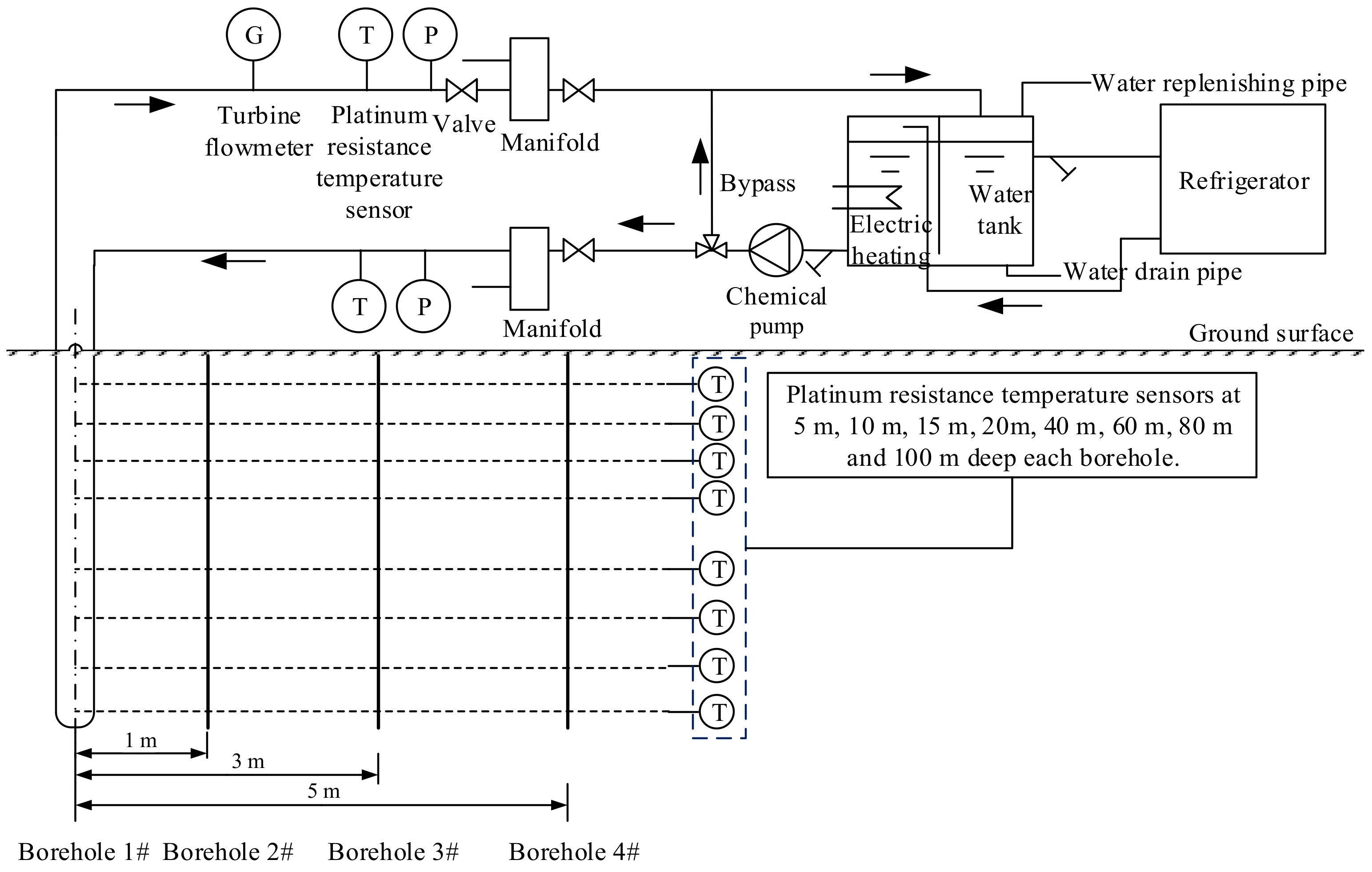
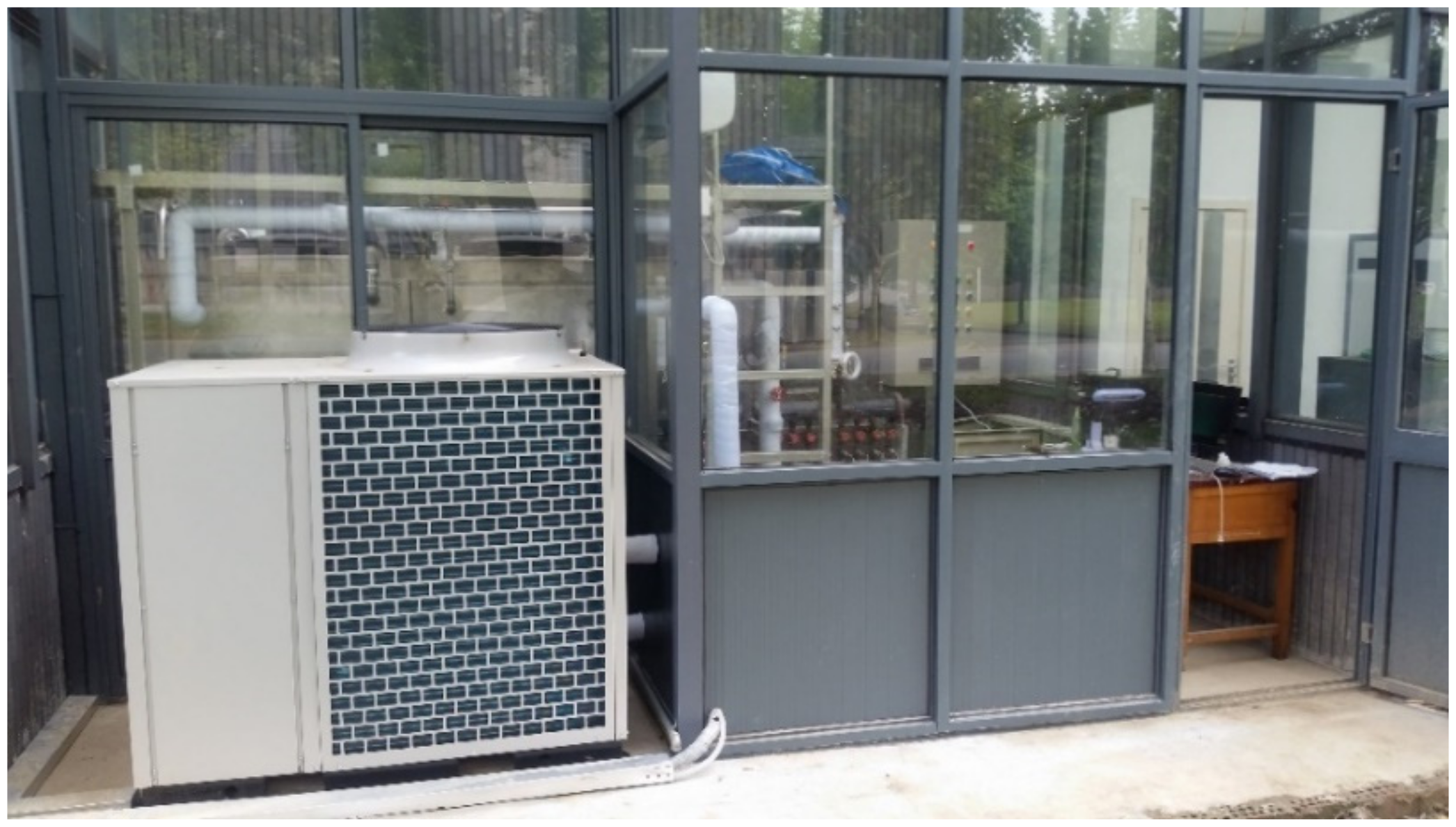
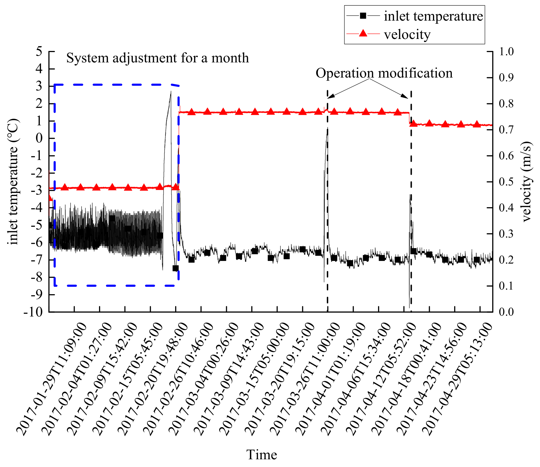
2.1. Experimental Set-Up

An experimental platform was established in Shanghai, China, to test GHE thermal performance. Figure 1 and Figure 2 show the diagram of the set-up and the equip room, respectively.

Chilled water-glycol was supplied by an air-cooled refrigerator. The refrigerator (HL-B50/4S, Join Technology, Guangzhou) could supply −7~0 °C water-glycol with a cooling capacity of 12 kW. The parameters of four vertical single U-tube GHE are listed in

Table 1. Parameters of the tested U-tube ground heat exchangers (GHEs).

Pipe thermal conductivity	0.6 W/(m·K)
Pipe outside diameter	32 mm
Pipe inner diameter	25 mm
The diameter of the borehole	160 mm
Borehole length	100 m
Filling material around the pipe	Borehole soil

. The system also included a 3 m³ water tank, a chemical pump (LQ-15BEX, LEZQ, Kunshan) with a max flow rate of 60 L/min, and a data logger. To avoid freezing the pipes, an aqueous solution of ethylene glycol (30% by mass) was used as circulating fluid. PT100 temperature sensors with an accuracy of ±0.2 °C were installed. The sensors were calibrated via standard thermometer at every 5 °C step (from 0~40 °C) before implanted. The error of the turbine flowmeter (NFLWGY-15, Kunshan Soutec Instrument, Kunshan) was within ±1.0%.

By switching valves, flow only occurred in the pipes of borehole 1#, and the sensors in borehole 2#, 3#, and 4# recorded soil temperature variation simultaneously. The inlet and outlet temperature and flow rate of GHE were recorded every minute. As atmospheric temperature fluctuated in the three-month test, the refrigerator’s outlet temperature and the flowrate of GHE were adjusted to ensure the system operate under the designed working conditions. The system operated continuously from January 28th to April 28th, 2017. The supply temperature of the refrigerator ranged from −5~−7°C.

2.2. RC Model Development

One of the major works of this study is to develop an improved RC model with soil phase change module, so that the new model can analyze GHEs heat transfer performance under normal and freezing soil conditions.

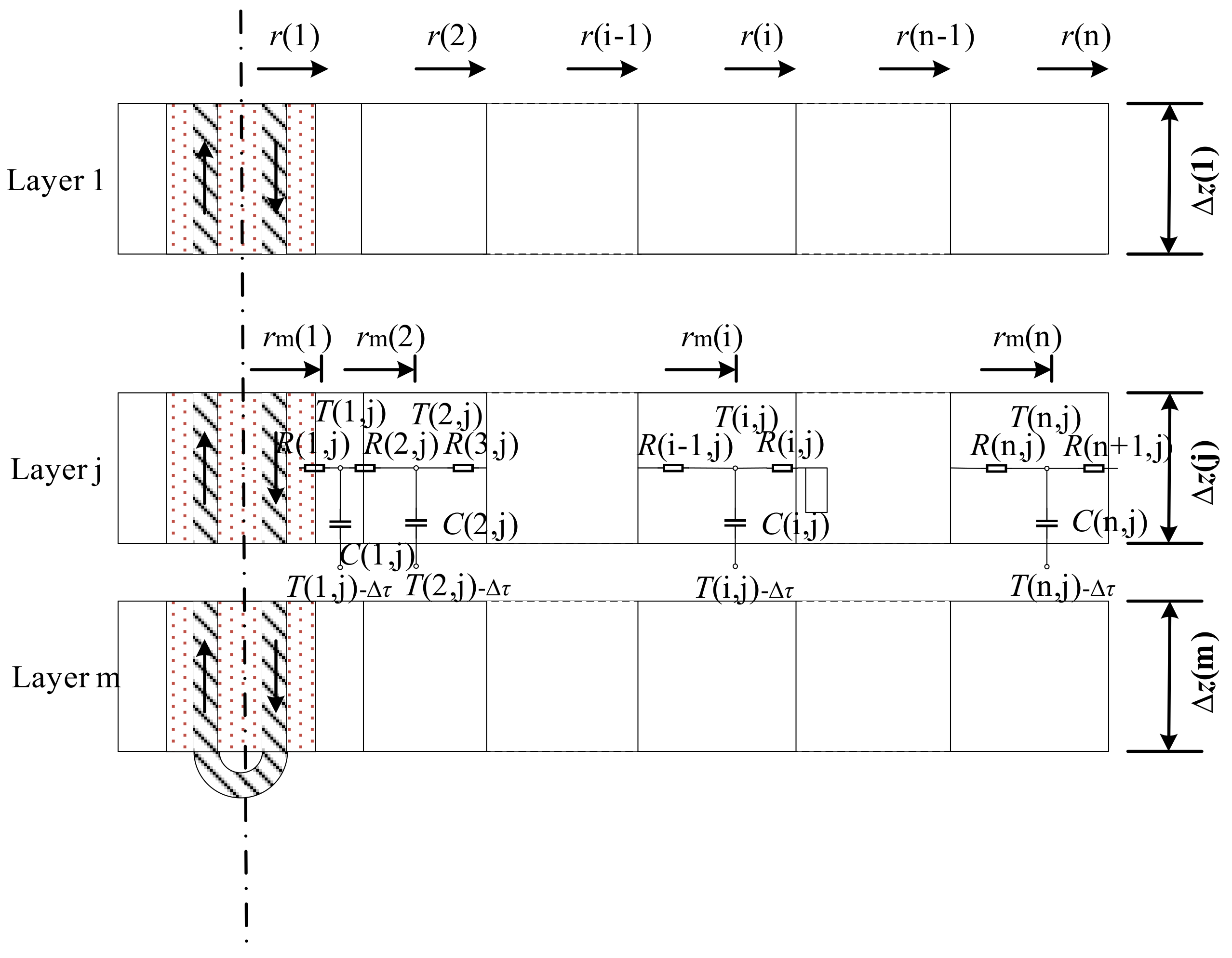
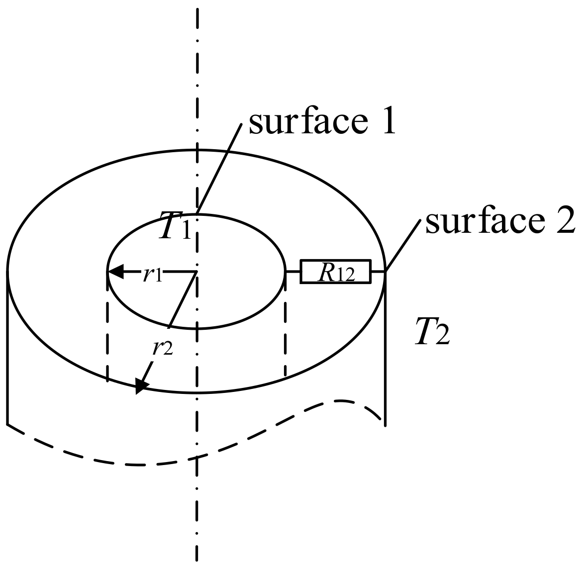
2.2.1. General RC Model

According to Fourier’s law, the thermal resistance for heat conduction through a circular pipe wall (see Figure 3) can be written as Equation (1). Where L is the length of the cylinder, λ is the thermal conductivity of the circular pipe wall, r₁ and r₂ are the inner and the outer pipe radius.

$$R_{12}=\frac{1}{2\pi L\lambda }\ln (\frac{r_2}{r_1})$$

(1)

By ignoring the temperature gradients, the heat flux q at the surface of a controlled thermal-storing body is Equation (2), where ρ c V is the heat capacity of the control body.

$$q=\rho cV\frac{dT}{d\tau }$$

(2)

The energy balance equation for three adjacent nodes i−1, i and i+1 (see Figure 4), can be described as Equation (3). Using finite time steps ∆τ, Equation (3) becomes Equation (4). Where R(i−1, i) is the thermal resistance between node i−1 and node i, T(i)_−Δτ is the temperature at node i for the previous time step.

$$q(i-1,i)+q(i,i+1)=\rho (i)c(i)V(i)\frac{dT(i)}{d\tau }$$

(3)

$$\frac{T(i-1)-T(i)}{R(i-1,i)}+\frac{T(i+1)-T(i)}{R(i,i+1)}=\frac{\rho (i)c(i)V(i)}{\Delta \tau }[T(i)-T{(i)}_{-\Delta \tau }]$$

(4)

2.2.2. Soil RC model

The soil boundary condition is related to the local climate. However, given that GHEs are often more than 50m deep from the ground surface, the influence of climate at that depth can be negligible.

The maximum radius (r_max) that the pipes can affect the soil is assumed. When the radius at a given time is greater than r_max, the soil temperature is assumed to be equivalent to ground temperature (T_o). The r_max is mainly related to the thermal diffusivity of the soil and the operation time. It can be calculated from the line-source model. According to previous studies, r_max can be assumed as 8~10 m. The effect of groundwater flow in the soil plays an important role in determining the GHE heat transfer under freezing soil conditions [22]. However, since groundwater flow is a site-specific issue, it is not considered in this study. The initial soil (and borehole) temperature is assumed to be the annual average soil temperature.

The 3-D soil body can be divided into m layers vertically and n rings horizontally. The thickness of each layer is Δz. Considering the following four reasons, we ignored the heat transfer between vertical layers to simplify the model. First, the pipe is the main heat source and sink, the heat transfer in the horizontal direction is much more significant than that in the vertical direction. Second, the soil around boreholes is a relatively small part of the whole ground, so that the soil heterogeneity difference has limited influences on heat transfer. Third, when we validate the RC model with the CFD model (see Section 3.1) that considered the vertical heat transfer, we found the heat transfer between vertical layers is neglectable. Forth, the simplified model costs much less computing time, which makes it easier for engineering use. By utilizing the symmetry of the cylinder, the model can be simplified to a two-dimensional model, as shown in Figure 5.

The energy balance for the j-th (0 < j < m) layer and i-th (0 < i < n) ring can be expressed as Equation (5). Where T(i,j) is the current mean temperature, T(i,j)_−Δτ is the mean temperature at the previous time step. R(i,j) means thermal resistance between two adjacent regions, C(i,j) is the soil thermal capacity, and they can be found in Appendix A. For the phase-changing region (i = n), considering the boundary condition and the ground temperature, Equation (5) becomes Equation (6). According to Equations (5) and (6), n equations can be assigned to each soil layer.

$$\frac{T(i-1,j)-T(i,j)}{R(i,j)}+\frac{T(i+1,j)-T(i,j)}{R(i+1,j)}=C(i,j)\frac{[T(i,j)-T{(i,j)}_{-\Delta \tau }]}{\Delta \tau }$$

(5)

$$\frac{T(n-1,j)-T(n,j)}{R(n,j)}+\frac{T_{\mathrm{o}}-T(n,j)}{R(n+1,j)}=C(n,j)\frac{[T(n,j)-T{(n,j)}_{-\Delta \tau }]}{\Delta \tau }$$

(6)

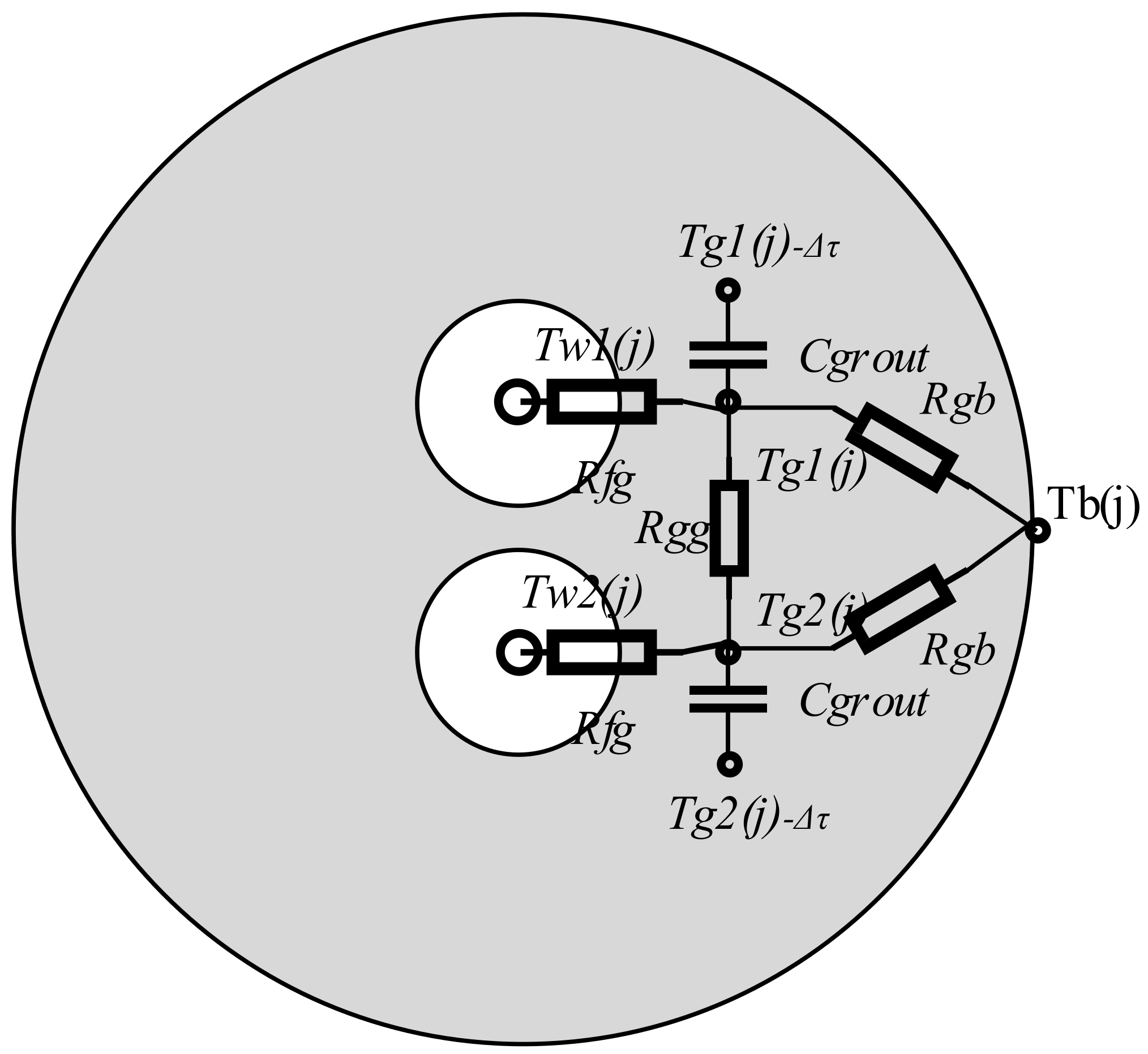
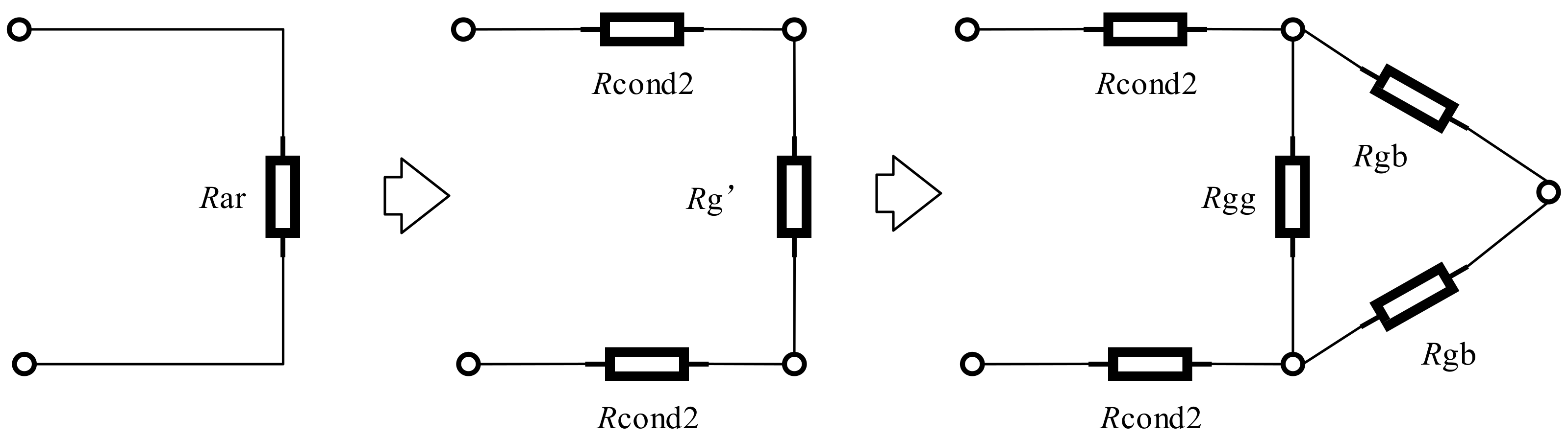
2.2.3. Borehole and Pipes’ RC Model

Locations of supply and return pipes at the same depth are symmetric, but their temperatures are not. As a result, the model inside the borehole cannot be simplified to two-dimensional, so that we propose a 5R2C model shown in Figure 6. Where T_w1(j) and T_w2(j) are the mean fluid temperature of supply and return pipes in the j-th section. T_g1(j) and T_g2(j) are the grout temperature of supply and return pipes surrounding the j-th section. T_b(j) is the j-th layer’s temperature of the borehole wall. R_fg(j) means thermal resistance among fluid and grout. R_gg(j) means thermal resistance between two grout sections. R_gb(j) stands for thermal resistance between grout and borehole wall, C_grout(j) means grout thermal capacity. More detailed information on these RC models for borehole can be found in Appendix A.

Borehole node equations

For the grout nodes that surround the supply pipe, we have:

$$\frac{T_{\mathrm{w}1}(j)-T_{\mathrm{g}1}(j)}{R_{\mathrm{fg}}}+\frac{T_{\mathrm{g}2}(j)-T_{\mathrm{g}1}(j)}{R_{\mathrm{gg}}}+\frac{T_{\mathrm{b}}(j)-T_{\mathrm{g}1}(j)}{R_{\mathrm{gb}}}=C_{\mathrm{grout}}(j)\frac{T_{\mathrm{g}1}(j)-T_{\mathrm{g}1}{(j)}_{-\Delta \tau }}{\Delta \tau }$$

(7)

For the grout nodes that surround the return pipe, we have:

$$\frac{T_{\mathrm{w}2}(j)-T_{\mathrm{g}2}(j)}{R_{\mathrm{fg}}}+\frac{T_{\mathrm{g}1}(j)-T_{\mathrm{g}2}(j)}{R_{\mathrm{gg}}}+\frac{T_{\mathrm{b}}(j)-T_{\mathrm{g}2}(j)}{R_{\mathrm{gb}}}=C_{\mathrm{grout}}(j)\frac{T_{\mathrm{g}2}(j)-T_{\mathrm{g}2}{(j)}_{-\Delta \tau }}{\Delta \tau }$$

(8)

For the nodes on the borehole wall, we have:

$$\frac{T(1,j)-T_{\mathrm{b}}(j)}{R(1,j)}+\frac{T_{\mathrm{g}1}(j)-T_{\mathrm{b}}(j)}{R_{\mathrm{gb}}}+\frac{T_{\mathrm{g}2}(j)-T_{\mathrm{b}}(j)}{R_{\mathrm{gb}}}=0$$

(9)

Heat balance equation

The following equation links the temperature of two layers:

$$T_{\mathrm{w},\mathrm{out}}(j)=T_{\mathrm{w},\mathrm{in}}(j+1)$$

(10)

For j = m, the above equation becomes:

$$T_{\mathrm{w}1}(m+1)=T_{\mathrm{w}2}(m+1)$$

(11)

The heat transfer between the fluid and the pipe at each layer is:

$$m_{\mathrm{w}}{c}_{\mathrm{pw}}[T_{\mathrm{w},\mathrm{in}}(j)-T_{\mathrm{w},\mathrm{out}}(j)]=\frac{{\overline{T}}_{\mathrm{w}}(j)-T_{\mathrm{g}}(j)}{R_{\mathrm{fg}}}\Delta z$$

(12)

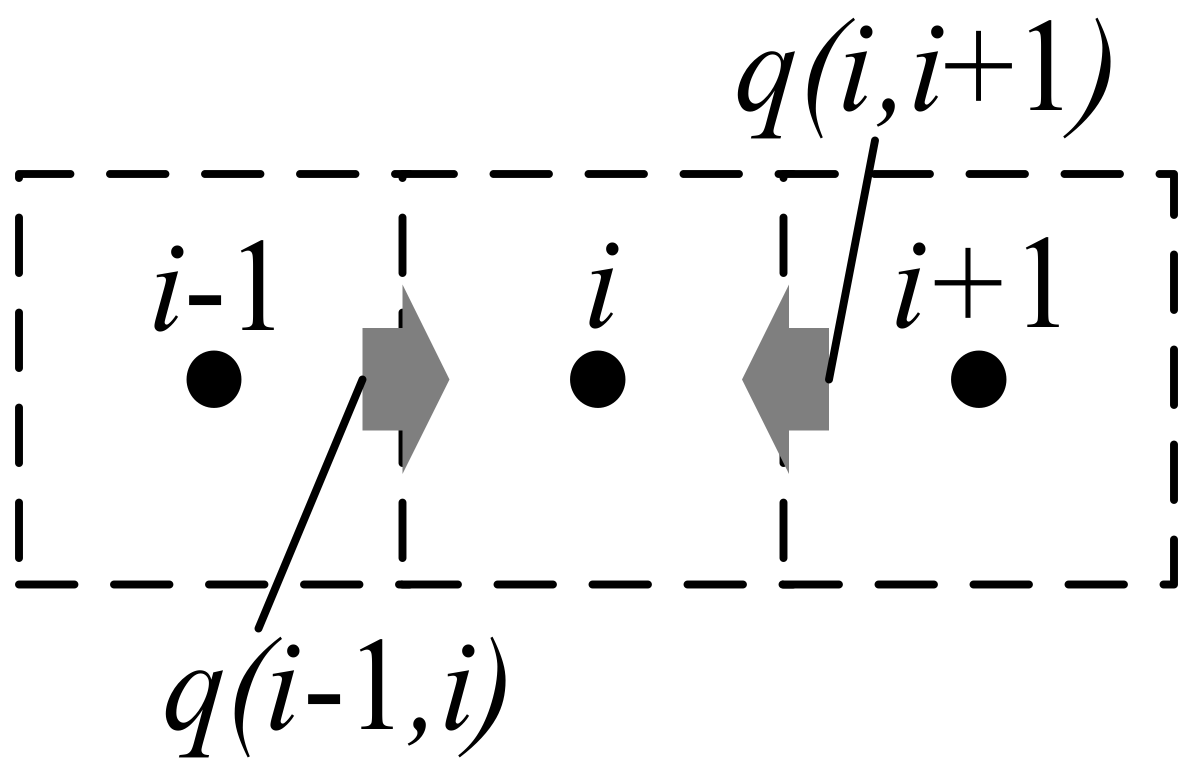
2.2.4. Model Solving

According to Equations (7) to (12), there are m layers. Each layer consists of n nodes outside the borehole and 5 nodes inside the borehole. In total, there are (5 + n) × m of nodes and equations. Additionally, input parameters for the model at every time step include soil temperature, inlet temperature T_w1 (1) and flow speed v.

The problem can be regarded as solving a group of linear equations, which can be converted into a matrix equation as Equation (13). [A] is a sparse matrix of temperature nodes coefficients. [T] is a column vector of node temperature. [B] is a column vector of constants.

[A] [T] = [B]

(13)

2.2.5. Module for Freezing Condition

The RC model derived in this paper can be used for GHEs simulation under normal conditions. For freezing soil conditions, a module for the freezing conditions is added accordingly to analyze the heat transfer characteristics.

Latent heat can be regarded as a large heat capacity in a small temperature change. Specific heat and thermal conductivity at the range of T_m-ΔT ≤ T_m ≤ T_m + ΔT are calculated respectively using the following equations [22]. Where λ_fr and λ_ufr are conductivities, C_fr and C_ufr are the volume heat capacity, ∆T is a small temperature increment, H is liquid latent heat. W is soil moisture content. ρ is material’s density and C is mass heat capacity.

$$\lambda =\left\{\begin{array}{ccc}\hfill {\lambda }_{\mathrm{fr}}& & (T<T_{\mathrm{m}}-\Delta T)\hfill \\ \hfill {\lambda }_{\mathrm{fr}}+(T-T_{\mathrm{m}}+\Delta T)\frac{{\lambda }_{\mathrm{ufr}}-{\lambda }_{\mathrm{fr}}}{2\Delta T}& & (T_{\mathrm{m}}-\Delta T\le T\le T_{\mathrm{m}}+\Delta T)\hfill \\ \hfill {\lambda }_{\mathrm{ufr}}& & (T>T_{\mathrm{m}}+\Delta T)\hfill \end{array}\right.$$

(14)

$$C=\left\{\begin{array}{ccc}\frac{C_{\mathrm{fr}}}{\rho }& & (T<T_{\mathrm{m}}-\Delta T)\hfill \\ \frac{H·W}{2\Delta T}+\frac{C_{\mathrm{ufr}}+C_{\mathrm{fr}}}{2\rho }& & (T_{\mathrm{m}}-\Delta T\le T\le T_{\mathrm{m}}+\Delta T)\hfill \\ \frac{C_{\mathrm{ufr}}}{\rho }& & (T>T_{\mathrm{m}}+\Delta T)\hfill \end{array}\right.$$

(15)

The physical properties of the clayey soil are [22]:

$${\lambda }_{\mathrm{fr}}=0.104\times {10}^{-3}{\rho }^{0.921}+3.721\times {10}^{-5}\rho W$$

(16)

$${\lambda }_{\mathrm{ufr}}=0.408\times {10}^{-3}{\rho }^{0.945}+1.72\times {10}^{-5}\rho W$$

(17)

$$C_{\mathrm{fr}}=\rho (0.914+0.023W)·1000$$

(18)

$$C_{\mathrm{ufr}}=\rho (0.815+0.041W)·1000$$

(19)

The freezing condition module is embedded in the calculation program so that it can be called when needed. When the temperature is below 0 °C, Equations (16) to (19) would be used to calculate the corresponding heat capacity and conductivity under frozen conditions.

2.2.6. Inputs and Outputs for RC Model

The inlet temperature and flow rate can be used as the input parameters for the RC model. Then, the output of the model, such as the outlet temperature, can be verified using the experimental results. The maximum radius, r_max, was set to 10 m. Compared with the three-month experiment, the simulation time step was set as 600 s. Other soil thermophysical parameters are summarized in

Table 2. Soil thermophysical parameters.

Parameters	Value
Density [kg/m3]	1925
Moisture content	40%
Volumetric heat capacity [J/(m3·K)]	3,936,600 (unfrozen)	3,087,700 (frozen)
Conductivity [W/(m·K)]	1.84 (unfrozen)	2.98 (frozen)

.

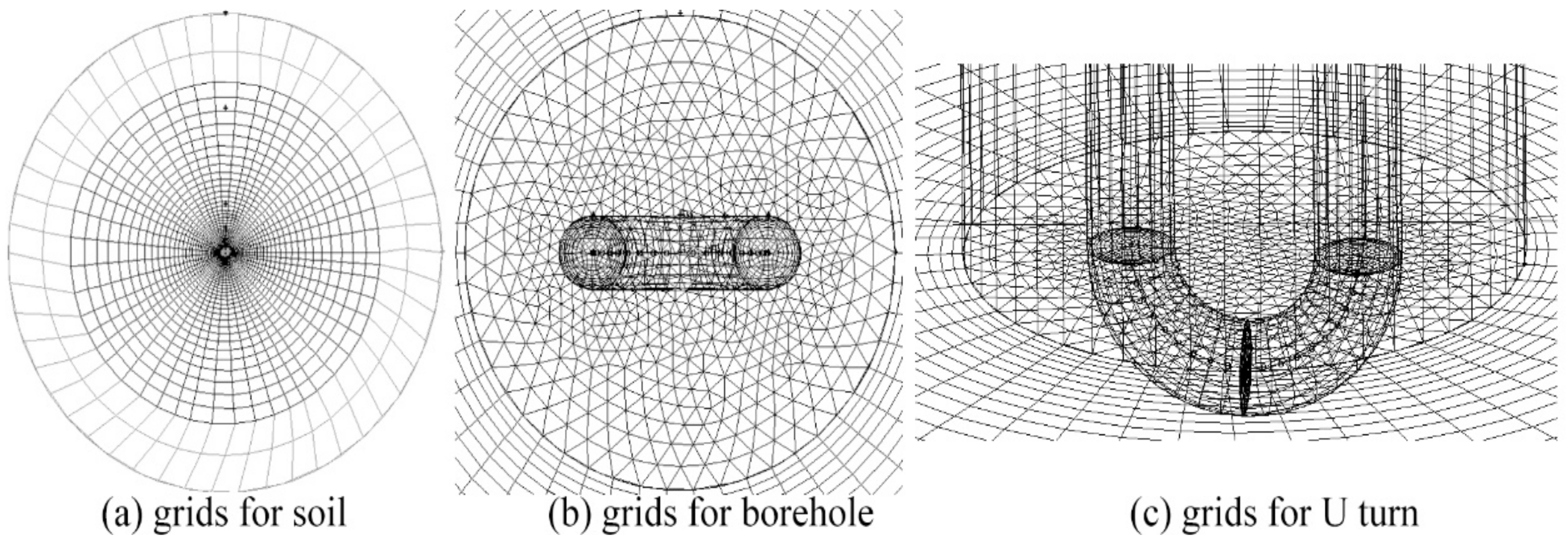
2.3. CFD Model Description

CFD method was used to validate the RC model from perspectives of heat transfer and temperature distribution [24,25]. A three-dimensional discretized finite volume model (as Figure 7) was developed in GAMBIT. The horizontal cross-sections of the borehole and surrounding soil were represented by different cells. For the annular areas of the soil, regularly shaped quadrilateral cells were adopted, while the irregular grout areas were discretized using triangular cells. In total, there were 4,070,000 cells satisfying grid independence. The standard k-ε model in FLUENT software was adopted. The convergence residual of continuity, velocity, k, and epsilon was set at 1E-3, and that of the energy residual was 1E-6.

A user-defined function on the effective heat capacity was compiled to Fluent to provide the ability to solve the frozen problem. The materials and boundary conditions were set according to experimental setups (described in Section 2.1). The simulation was in a transient state with 1800 s of time step (i.e., the measured inlet temperature and flow speed were introduced to the CFD model every 30 min). Given that the major focus of this study is the RC-model development and the CFD model was only built for validation purposes. We, therefore, streamlined the description of the CFD model here.

3. Results and Discussion

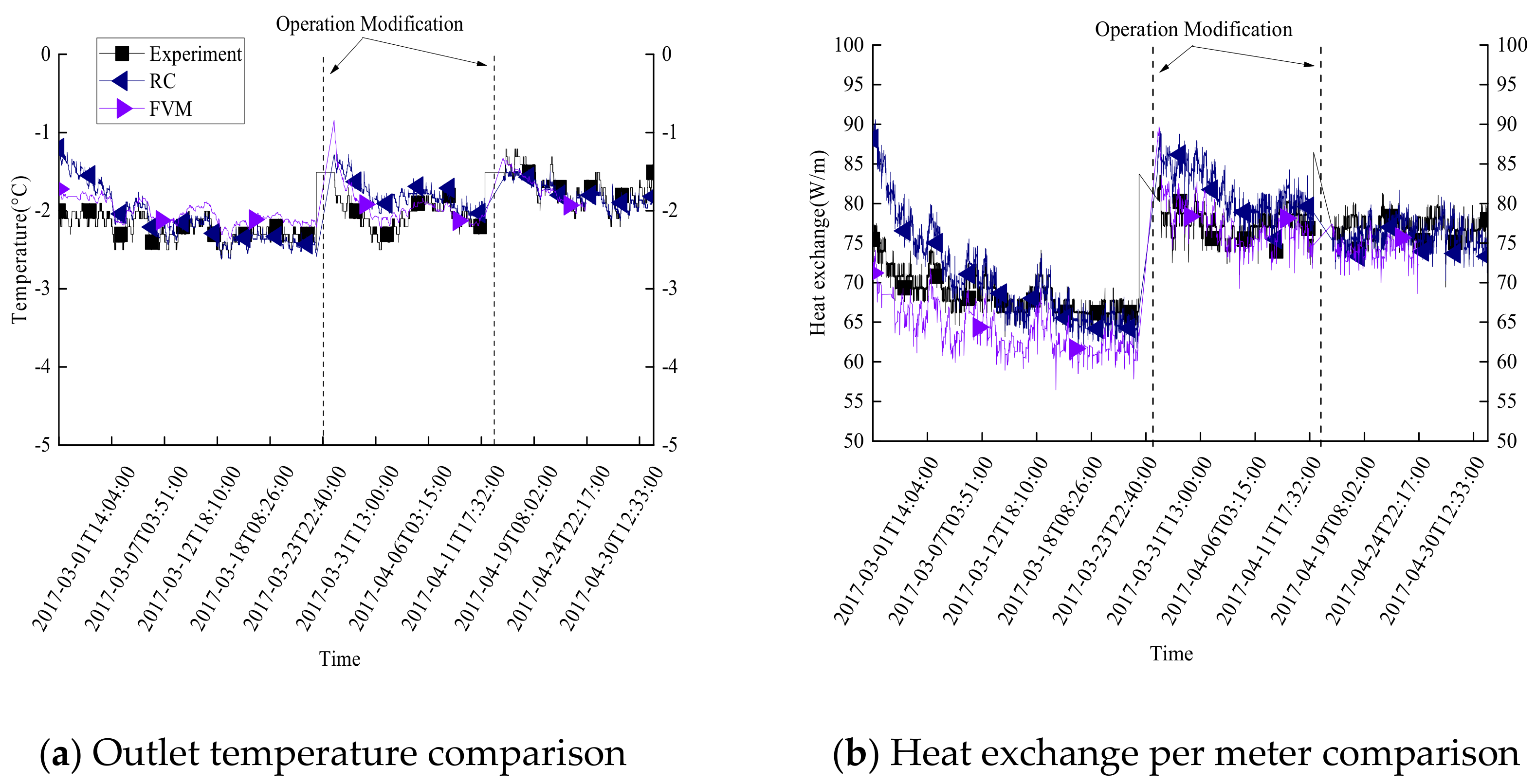
3.1. RC Model Validation

3.1.1. Heat Exchange Validation

Figure 8 shows the measured GHE inlet temperature and velocity. These two variables are input parameters for the RC model and CFD method. The outlet temperature of the refrigerator was unstable during the first month because of commissioning. However, it was maintained within 2 °C variances in the following months. We excluded the first-month data when doing the analysis.

Table 3. The temperature along the operating pipes at the end of the test.

Depth underground (m)	5	10	15	20	40	60	80	100
Temperature (°C)	−2.6	−3.0	−3.8	−2.4	−1.5	−2.6	−2.1	−0.1

summarizes the temperature along the operating pipes at the end of the three-month test. The soil around the pipes has been frozen after three months because the measured temperatures were below the frozen point (0 °C).

The heat exchange performance is a crucial parameter for GSHP system design. Figure 9 compares the outlet temperature and heat exchange rate between the measured data, CFD results, and the RC model prediction. According to Figure 9, the heat exchange stabilized at 78 W/m during the third month. The minimum heat exchange rate during the whole three-month operation was 66 W/m, which means the frozen soil did not deteriorate GHE’s heat transfer performance. The GHE extracted heat from the soil continually and steady even with soil phase changes. This is very useful information for GHE application in cold or several cold climate zones because 12~77 W/m GHE heat transfer capacity can guarantee the normal operation of GSHP systems. The heat transfer improvement of frozen soil can actually help to reduce the GHE scale and initial cost.

When compared with the experimental measurement, the maximum and minimum errors in the heat exchange rate were 10% and 0.1% respectively for the RC model and 21% and 0.03% for the CFD model. The RC model only needs 3.5-h computing time, but it took the CFD solver 37 h to finish the calculation. From the perspectives of accuracy and computing time, the RC model has an advantage over the CFD model.

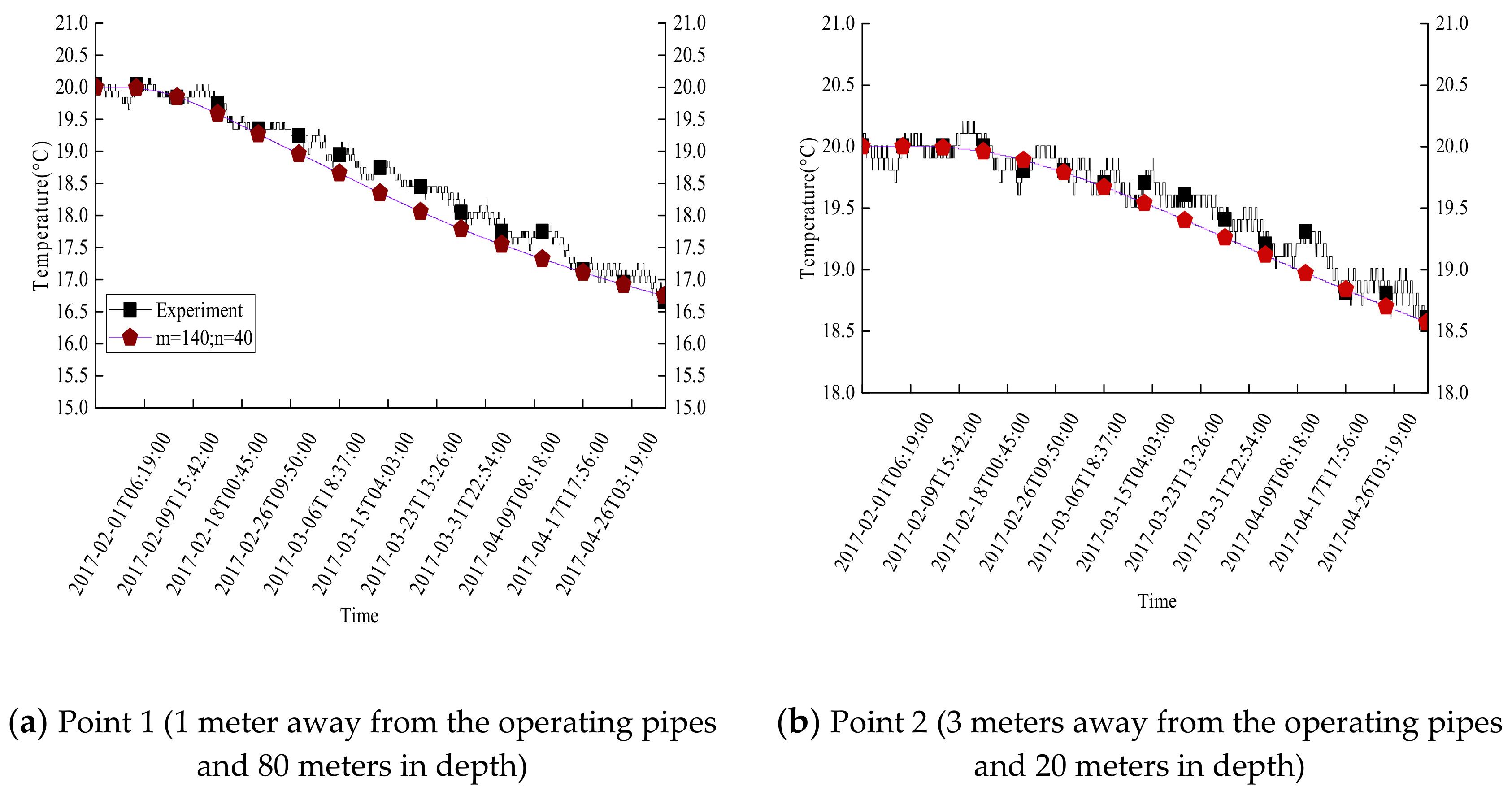
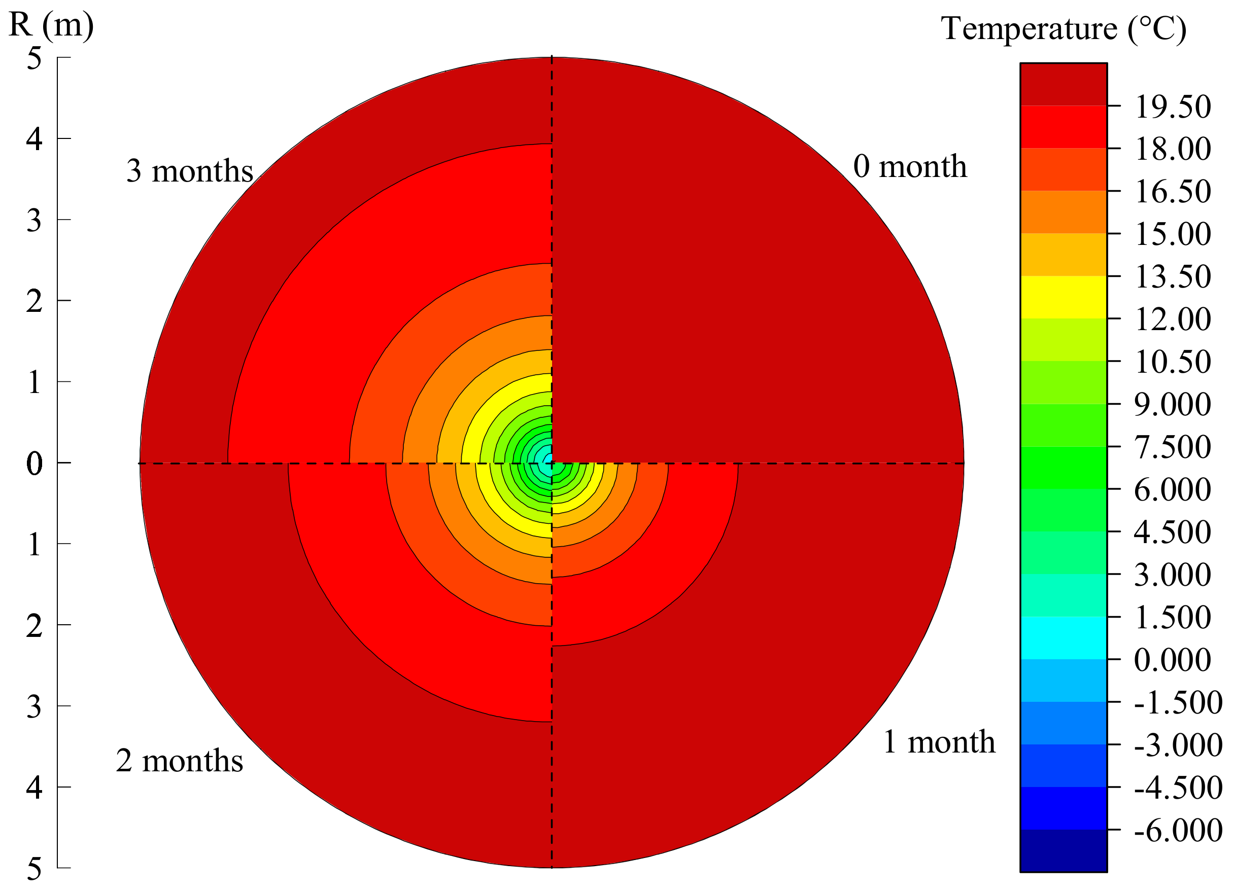
3.1.2. Temperature Distribution Validation

The soil temperature distribution can also be validated. According to Liu et al. [26], the soil depth with constant temperature depends on its thermal diffusivity. Normally, the depth should be 8~11 m. To exclude the influence of atmosphere temperature variance, the validating points should be deeper than 11 m. Point 1 and Point 2 (see Figure 1) were selected for these considerations.

As shown in Figure 10, the temperature at Point 1 dropped from 20.0 °C to 16.8 °C, and the temperature at Point 2 dropped from 20.0 °C to 18.6 °C after the three-month test. Point 1 has a larger temperature drop because it is closer to the GHE pipes. For the same reason, point 1 also takes less time to respond to the low input temperature of GHE pipes. The thermal capacity of the soil mass between the monitored points and the GHE pipe contributed to the delay in temperature changes.

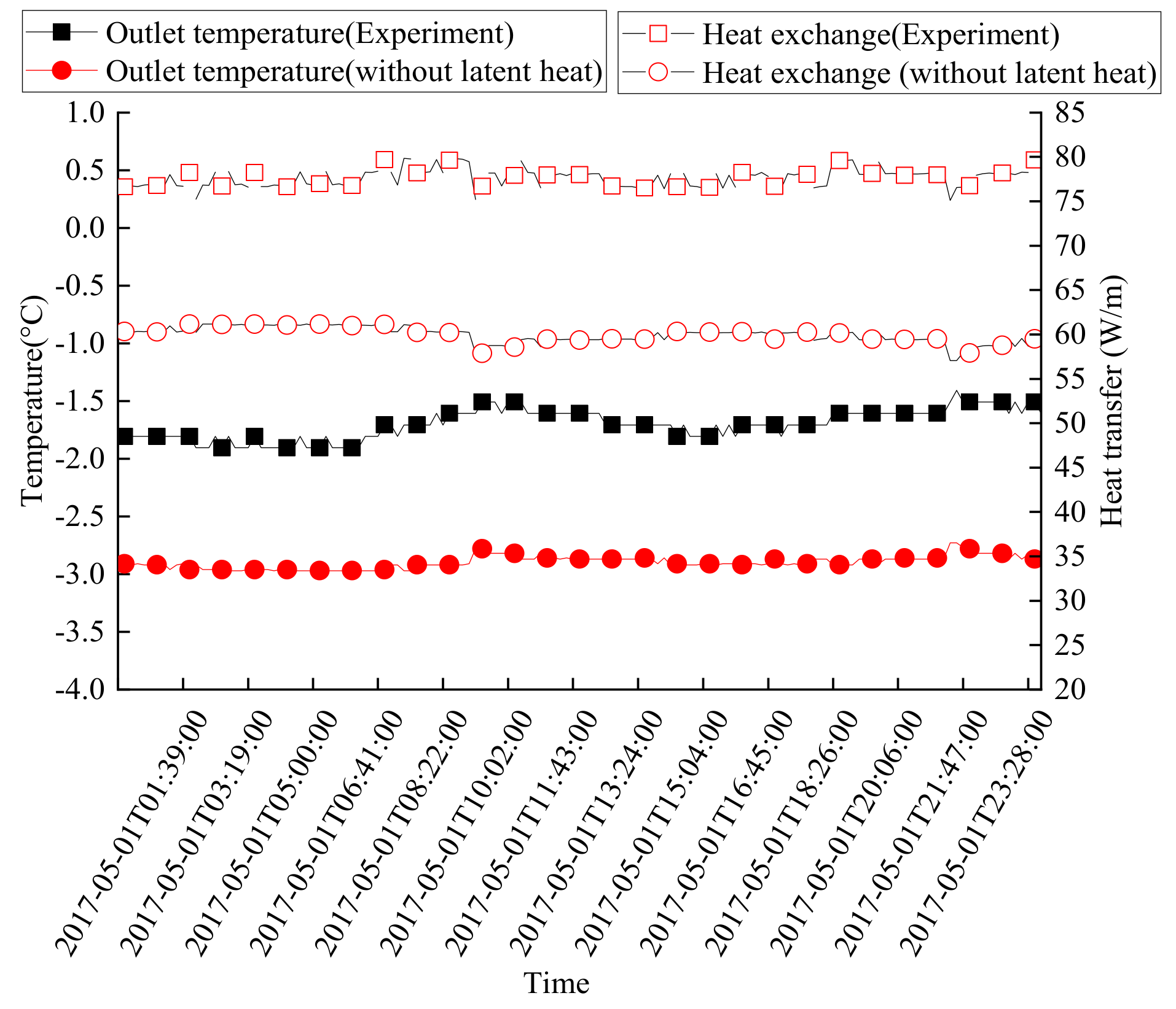
3.2. Freezing Soil and GHE Thermal Performance

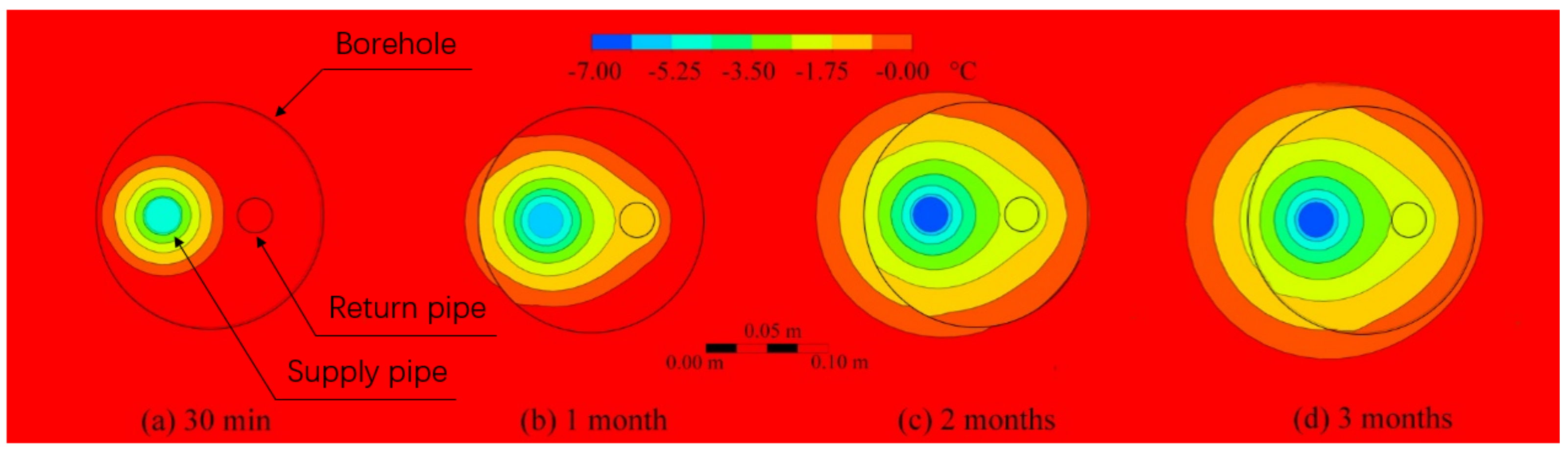
3.2.1. Effects on Temperature Distribution

The above validations show that the simulated results from the RC model matched well with the experimental results on both heat exchange rate and soil temperature distribution, which means the improved RC model is reliable for analyzing the temperature variation during the operation period. A slice of the RC model at 50 m depth was taken as an example to show how the soil temperature varied with the operation time.

Figure 11 shows the soil temperature distribution during the three-month simulation. It compares the temperature distributions at the initial state (0 months), 1st month, 2nd month and 3rd month. The result indicates that the low GHE inlet temperature can influence the soil temperature as far as 4 m after the three-month operation. The temperature difference between the initial soil temperature and GHE inlet temperature was 27 °C, which is the driven force for the heat transfer. After the three-month operation, the soil temperature decreased to 9.2 °C (60% of the initial temperature difference) and the affected radius was limited to 1m. This indicates that the freezing-temperature operation of GHE would not cause severe temperature perturbation on surrounding soil even after a three-month operation.

3.2.2. Effects on Frozen Zone

When the moisture (or water) in the soil around GHE pipes gets frozen, the thermal performance of GHE will be affected. Since the RC model simplifies the structure within the borehole, it is unable to show the temperature changes around the pipes directly. To analyze the changes in the frozen zone, Figure 12 shows the CFD simulation results at the slice of 15 m depth.

Figure 12 shows that the temperature of the grout around the supply pipe dropped more quickly than that around the return pipe. It takes a long time (> 1 month) for the soil around the borehole to get frozen. The affected frozen radius outside the borehole is less than 0.10 m. However, although the effects on frozen zone seem to be quite limited in this case, the value of the frozen radius in subsequent years may be expanded to an extent that cannot be ignored if intensive heat was extracted from the ground, especially when there is insufficient heat supplement or balance.

3.2.3. Effects on the Heat Transfer Rate

To evaluate the effect of soil freezing on the heat transfer rate of GHE, we compared the simulation results of the RC model without the freezing module. Figure 13 shows the comparisons of GHE outlet temperature and heat exchange rate during the last 24 h in the 3-month experiment.

As aforementioned, the experimental measurements showed the GHE heat exchange rate stayed at 75–80 W/m under frozen soil conditions, and the RC model with freezing module produced similar results. Figure 13 shows that the RC model without the freezing module predicted 1.2 °C and 17.7 W/m lower (averagely) in the outlet temperature and heat exchange rate than the measured results. These values suggest that the phase change of soil moisture/water can increase GHE’s heat transfer capacity. The specific increment in the test is as high as 30%, which can be considered as an advantage of GHE running in freezing inlet temperature. For real GHE applications in cold climate zones, the soil moisture content can be lower than our test condition (which was 40% soil moisture content), so that the improvement on heat transfer performance may be lower than the tested results. However, both the experimental results and simulated estimations indicate that the freezing soil condition will not deteriorate GHE’s heat transfer. This is very useful information for applying GHE under freezing soil conditions.

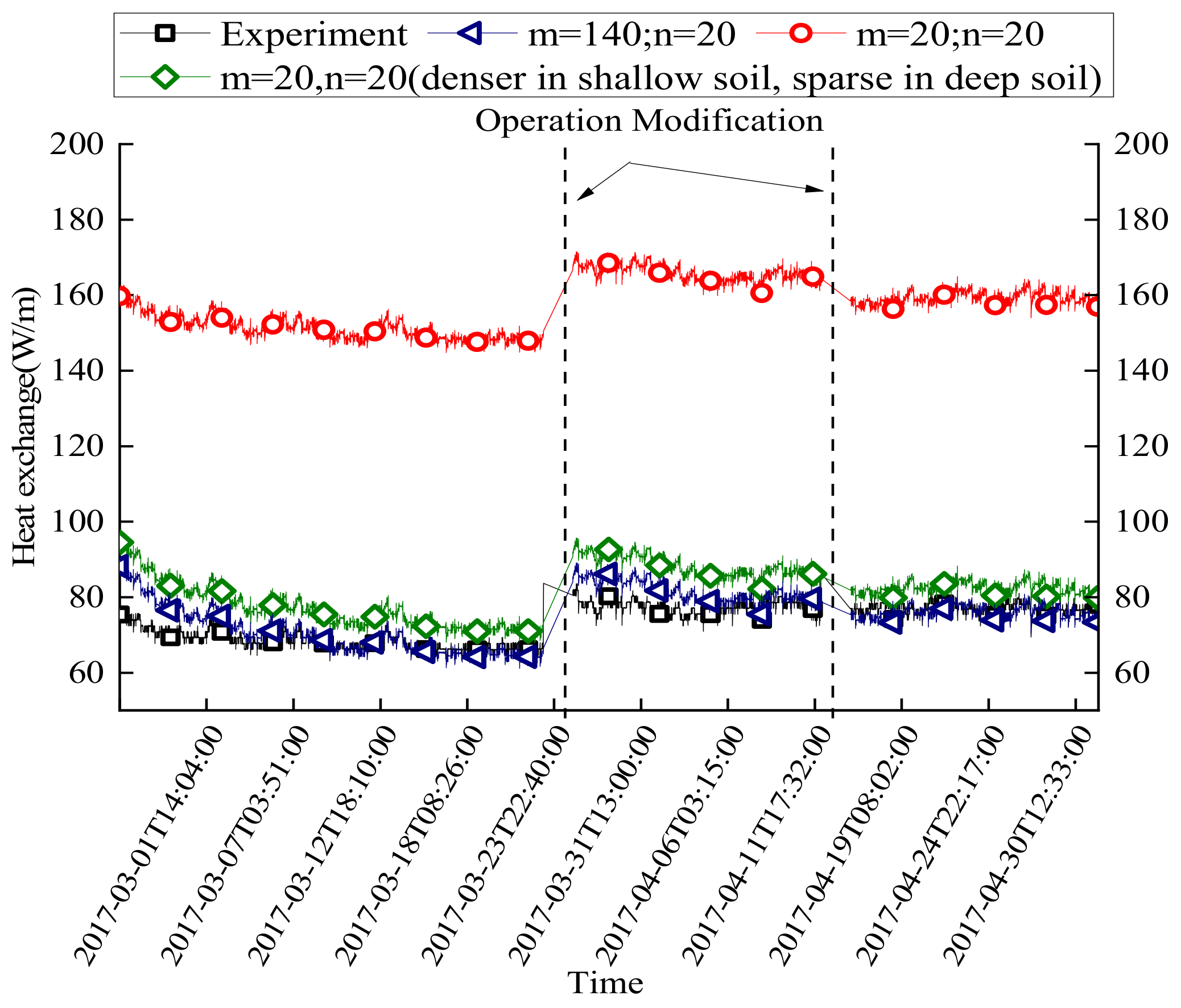
3.3. Model Optimization

The accuracy of the RC model depends on the m and n values, which stand for the numbers of vertical layers and horizontal rings of the soil model (see Figure 5). For averaged division method, the larger the m and n values, the better the simulation results would be. Since there are more calculation nodes. However, this will lead to a remarkable increase in computing load. To compromise the accuracy and computing time, we chose 140 m-layers and 20 n-rings in this study. We also tried the idea that dividing the soil into m layers but denser in shallow ground sand sparser in deep ground. Since the temperature and moisture changes are more significant in shallow soil, it would be better to put more calculation nodes there. In this way, the m value can be cut down to 20 without significant accuracy loss (see Figure 14).

3.4. Limitations

The modified RC model shows reliable results in predicting heat transfer of GHE under freezing soil conditions. There are three limitations should be noted. (1) The model is not able to directly give results on temperature distribution within the borehole because it is a simplified 5R2C-node model. However, it can be used to simulate the heat exchange and soil temperature distribution outside the borehole. (2) The current model is built for single U-tube GHE simulation. When applied to multiple GHEs, further modifications are needed, especially for the ununiformed boundary temperatures. (3) Although the GHE heat transfer capacity increased under freezing soil conditions, the COP of GSHP may decrease if the ground circulating water-glycol temperature is too low [27,28]. Future studies are needed to analyze how the enhanced GHE heat transfer and lowered circulating fluid temperature would collectively affect the overall efficiency of the GSHP system.

4. Conclusions

The heat transfer performance of ground heat exchangers (GHE) was studied under freezing soil conditions through experiment tests and model simulations. (1) An improved thermal resistance and capacity (RC) model was developed to analyze the heat transfer of a single U-tube GHE with the soil phase change module. The new model has been validated with experimental measurements and CFD results. With 140 vertical layers and 20 horizontal rings, the model can produce very reliable results (with < 10% error) without adding too much computing load. (2) The frozen soil can increase the GHE heat transfer capacity. Under the test condition, the soil phase change contributed to a 30% increase in GHE’s heat transfer capacity. Even after a three-month operation, the heat transfer capacity remained between 75~80 W/m, which is high enough to ensure ground source heat pump systems work properly in cold climate zones. (3) The GHE’s heat transfer rate remained at a relatively high level throughout the three-month test. GHE can continuously extract heat from the ground during the 3-month test. The impact of the frozen operation on soil temperature distribution is limited. The maximum influence radius is 4 m, while the frozen radius is only 0.1 m.

References

1. Xu, W.; Liu, Z. Development and Prospect of Ground Source Heat Pump Technology in China. Build. Sci. 2013, 29, 26–33. [Google Scholar]
2. Vasilyev, G.P.; Peskov, N.V.; Burmistrov, A.A.; Timofeev, N.A.; Zakharov, P.E.; Yurchenko, I.A. Ground Source Heat Pump Modeling: Accounting of Ground Moisture Freezing-Melting in a Model of Heat Transfer outside Deep Borehole. Appl. Mech. Mater. 2014, 704, 102–112. [Google Scholar] [CrossRef]
3. Ingersoll, L.R.; Plass, H.J. Theory of the ground pipe heat source for the heat pump. Heat. Pip. Air Cond. 1948, 54, 339–348. [Google Scholar]
4. Deerman, J.D. Simulation of Vertical U-tube Ground-coupled Heat Pump Systems using the Cylindrical Heat Source Solution. ASHRAE Trans. 1991, 97, 287–295. [Google Scholar]
5. Dahua, W.; Haifeng, Z.; Shuqiang, G. In Situ Test and the Analysis of Theoretical Applicability of Double U Type Pile Buried Tube Heat Exchanger. Geol. Sci. Technol. Inf. 2016, 35, 226–230. [Google Scholar]
6. Bernier, M.A. Ground-coupled heat pump system simulation. ASHRAE Trans. 2001, 107, 605–616. [Google Scholar]
7. Rottmayer, S.P.; Beckman, W.A.; Mitchell, J.W. Simulation of a single vertical U-tube ground heat exchanger in an infinite medium. ASHRAE Trans. 1997, 103, 651–659. [Google Scholar]
8. Muraya, N.K.; O’Neal, D.L.; Heffington, W.M. Thermal interference of adjacent legs in a vertical U-tube heat exchanger for a ground-coupled heat pump. ASHRAE Trans. 1996, 102, 12–21. [Google Scholar]
9. Yavuzturk, C.; Spitler, J.D.; Rees, S.J. A short time step response factor model for vertical ground loop heat exchangers. ASHRAE Trans. 1999, 105, 475–485. [Google Scholar]
10. Bai, L.; Wang, P.X. Simulation on Ground Temperature Change of GSHP System in Severe Cold Regions. Adv. Mater. Res. 2014, 945-949, 2820–2824. [Google Scholar] [CrossRef]
11. Shen, G.M.; Xu, Y.; Zhou, J.Y.; Hu, P.F.; Xiao, H. The Study of Soil Temputerature Change of GSHP System in Winter Conditions. Appl. Mech. Mater. 2013, 405–408, 2969–2974. [Google Scholar] [CrossRef]
12. Eskilson, P. Thermal Analysis of Heat Extraction Boreholes. Ph.D. Thesis, University of Lund, Lund, Sweden, September 1987. [Google Scholar]
13. Li, M.; Li, P.; Chan, V.; Lai, A.C.K. Full-scale temperature response function (G-function) for heat transfer by borehole ground heat exchangers (GHEs) from sub-hour to decades. Appl. Energy 2014, 136, 197–205. [Google Scholar] [CrossRef]
14. Hellström, G. Ground Heat Storage: Thermal Analysis of Duct Storage Systems. Ph.D. Thesis, University of Lund, Lund, Sweden, May 1991. [Google Scholar]
15. Sharqawy, M.H.; Mokheimer, E.M.; Badr, H.M. Effective pipe-to-borehole thermal resistance for vertical ground heat exchangers. Geothermics 2009, 38, 271–277. [Google Scholar] [CrossRef]
16. Carli, M.D.; Tonon, M.; Zarrella, A.; Zecchin, R. A computational capacity resistance model (CaRM) for vertical ground-coupled heat exchangers. Renew. Energy 2010, 35, 1537–1550. [Google Scholar] [CrossRef]
17. Zarrella, A.; Capozza, A.; Carli, M.D. Analysis of short helical and double U-tube borehole heat exchangers: A simulation-based comparison. Appl. Energy 2013, 112, 358–370. [Google Scholar] [CrossRef]
18. Bauer, D.; Heidemann, W.; Müller-Steinhagen, H.; Diersch, H.J.G. Thermal resistance and capacity models for borehole heat exchangers. Int. J. Energy Res. 2015, 35, 312–320. [Google Scholar] [CrossRef]
19. Pasquier, P.; Marcotte, D. Short-term simulation of ground heat exchanger with an improved TRCM. Renew. Energy 2012, 46, 92–99. [Google Scholar] [CrossRef]
20. Maestre, I.R.; Gómez, P.Á.; Pérez-Lombard, L. A new RC and g-function hybrid model to simulate vertical ground heat exchangers. Renew. Energy 2015, 78, 631–642. [Google Scholar] [CrossRef]
21. Kurylyk, B.L.; Hayashi, M. Improved Stefan Equation Correction Factors to Accommodate Sensible Heat Storage during Soil Freezing or Thawing. Permafr. Periglac. Processes 2016, 27, 189–203. [Google Scholar] [CrossRef]
22. Tian, B. Research on Operation Characteristic of Ground Heat Exchanger for Ground Coupled Heat Pump System in Cold Climate. Ph.D. Thesis, Harbin Institute of Technology, Harbin, China, June 2010. [Google Scholar]
23. Zheng, T.; Shao, H.; Schelenz, S.; Hein, P.; Vienken, T.; Pang, Z.; Kolditz, O.; Nagel, T. Efficiency and economic analysis of utilizing latent heat from groundwater freezing in the context of borehole heat exchanger coupled ground source heat pump systems. Appl. Therm. Eng. 2016, 105, 314–326. [Google Scholar] [CrossRef]
24. Congedo, P.M.; Colangelo, G.; Starace, G. CFD simulations of horizontal ground heat exchangers: A comparison among different configurations. Appl. Therm. Eng. 2012, 33–34, 24–32. [Google Scholar] [CrossRef]
25. Flaga-Maryanczyk, A.; Schnotale, J.; Radon, J.; Was, K. Experimental measurements and CFD simulation of a ground source heat exchanger operating at a cold climate for a passive house ventilation system. Energy Build. 2014, 68, 562–570. [Google Scholar] [CrossRef]
26. Liu, X.; Zhao, J.; Shi, C.; Zhao, B. Study on soil layer of constant temperature. Acta Energ. Sol. Sin. 2007, 28, 494–498. [Google Scholar]
27. Wu, W.; Wang, B.; You, T.; Shi, W.; Li, X. A potential solution for thermal imbalance of ground source heat pump systems in cold regions: Ground source absorption heat pump. Renew. Energy 2013, 59, 39–48. [Google Scholar] [CrossRef]
28. You, T.; Wu, W.; Shi, W.; Wang, B.; Li, X. An overview of the problems and solutions of soil thermal imbalance of ground-coupled heat pumps in cold regions. Appl. Energy 2016, 177, 515–536. [Google Scholar] [CrossRef]
Figure 1. Diagram of the experimental system.
Sustainability 11 05738 g001
Figure 2. Equipment room.
Sustainability 11 05738 g002
Figure 3. Thermal resistance model for two surfaces.
Sustainability 11 05738 g003
Figure 4. Nodes in the control body.
Sustainability 11 05738 g004
Figure 5. Resistance and capacity (RC) model for soil.
Sustainability 11 05738 g005
Figure 6. RC model for the borehole.
Sustainability 11 05738 g006
Figure 7. Model geometry and mesh for U-tube GHE and surrounding soil.
Sustainability 11 05738 g007
Figure 8. Inlet temperature and velocity.
Sustainability 11 05738 g008
Figure 9. Outlet temperature and heat exchange per meter comparison.
Sustainability 11 05738 g009
Figure 10. Temperature changes with time.
Sustainability 11 05738 g010
Figure 11. Soil temperature distribution at 50 m in depth.
Sustainability 11 05738 g011
Figure 12. The frozen zone around pipes.
Sustainability 11 05738 g012
Figure 13. Comparison between experiment and simulation without freezing module.
Sustainability 11 05738 g013
Figure 14. Comparison between simulation with different m and n.
Sustainability 11 05738 g014