Performance Evaluation of the GIS-Based Data-Mining Techniques Decision Tree, Random Forest, and Rotation Forest for Landslide Susceptibility Modeling


Abstract
1. Introduction
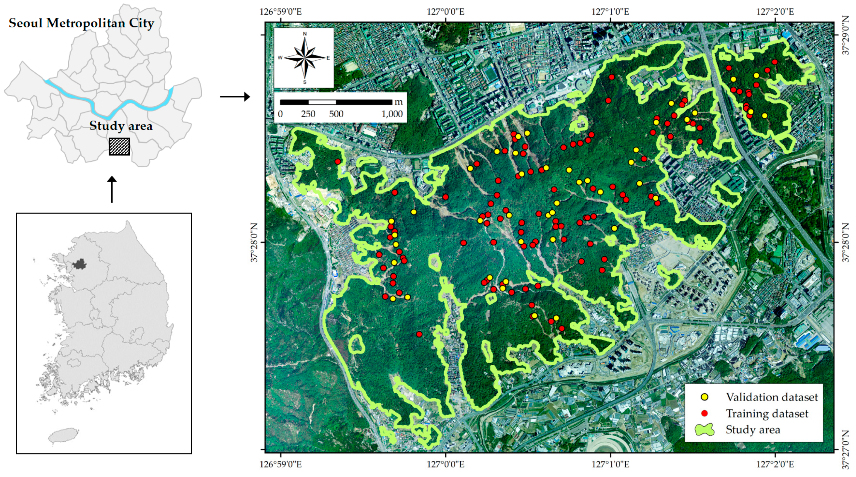
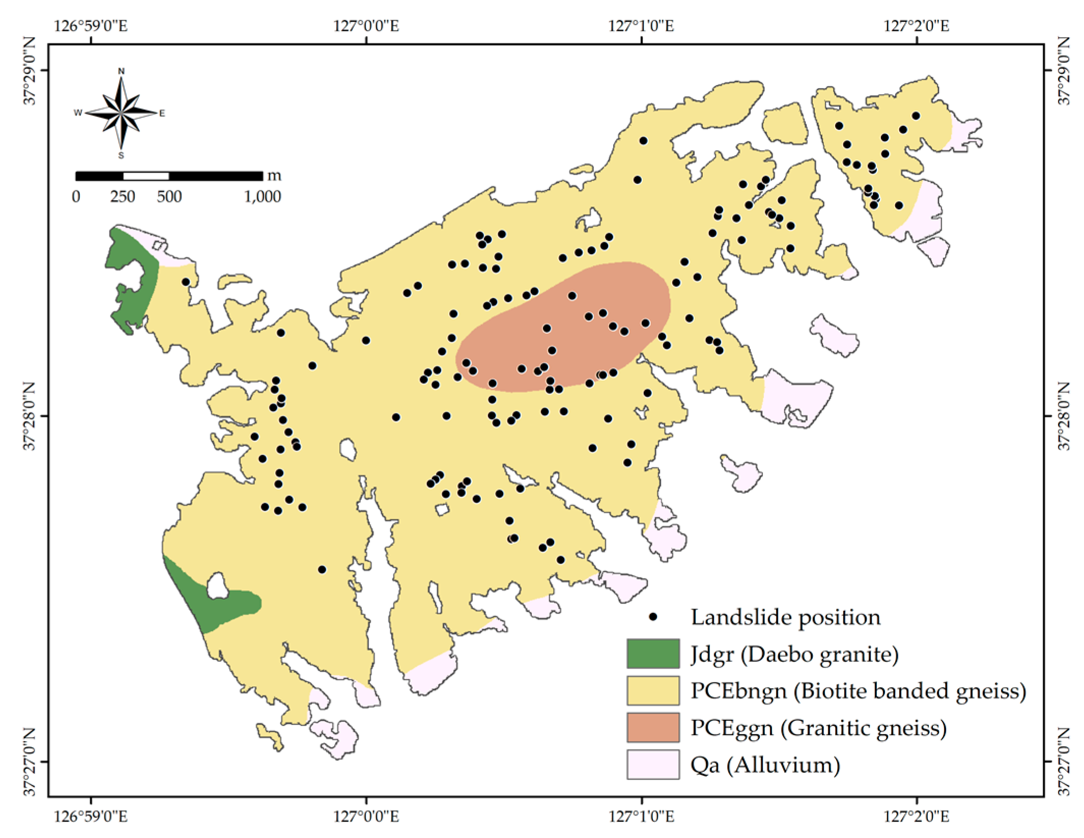
2. Study Area
3. Methodology
3.1. Construction of the Spatial Database
3.1.1. Landslide Inventory Map
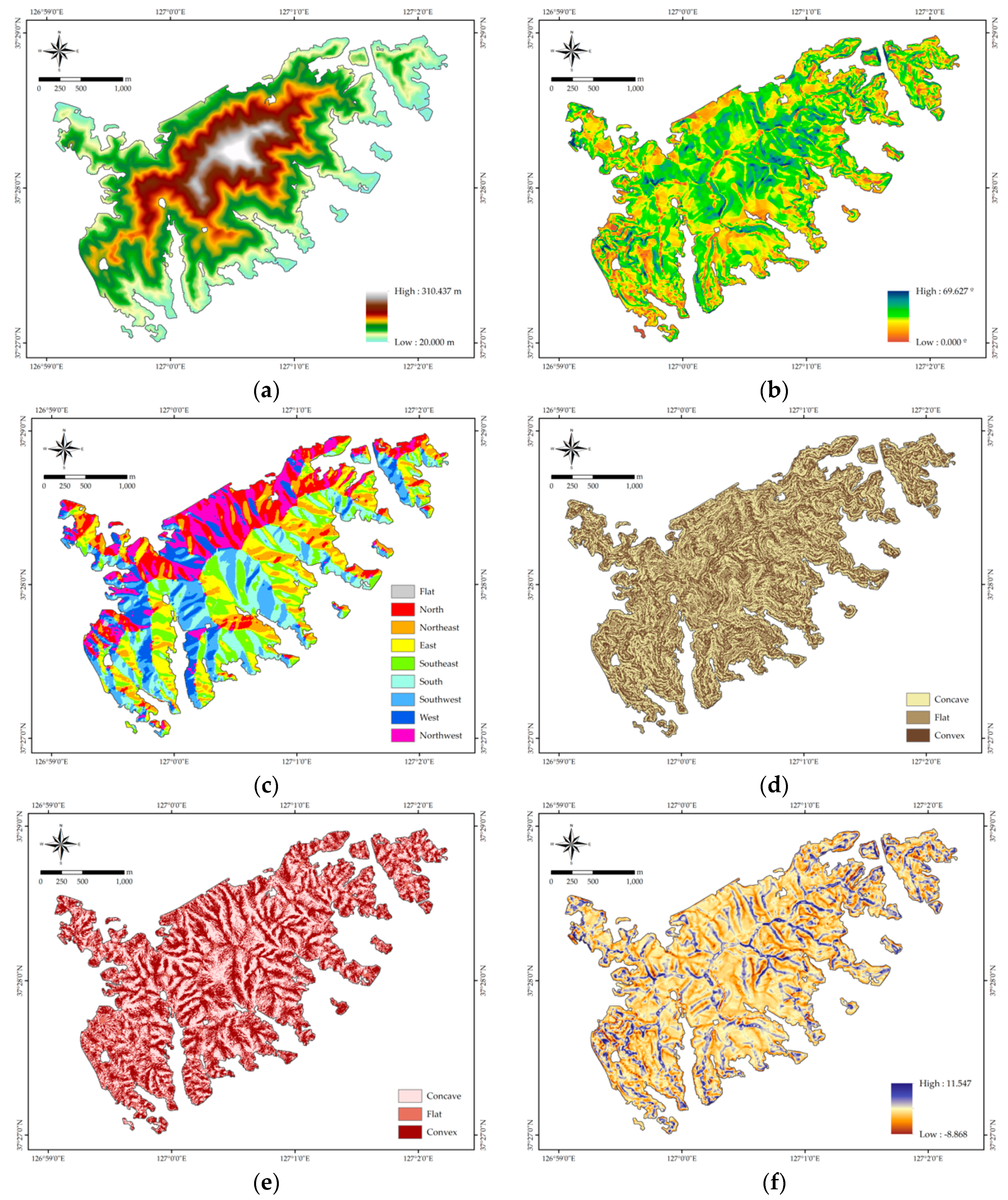
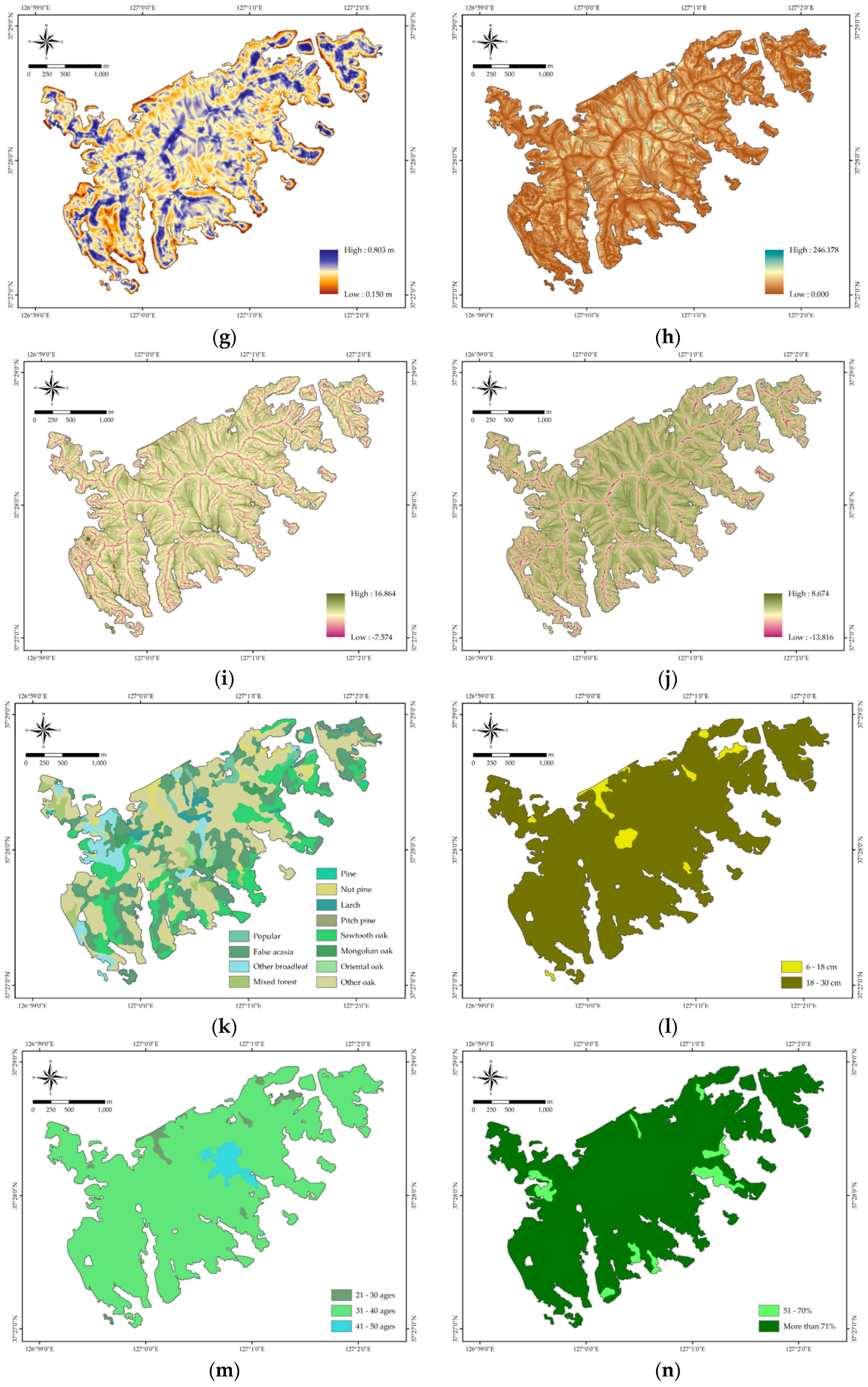
3.1.2. Landslide Conditioning Factors
3.2. Preparation of Training and Validation Datasets
3.3. Relief-F Feature Selection Method
3.4. Landslide Susceptibility Modeling
3.4.1. Decision Trees
3.4.2. Random Forest
3.4.3. Rotation Forest
3.5. Model Performance Assessment
4. Results
4.1. Landslide Conditioning Factor Analysis
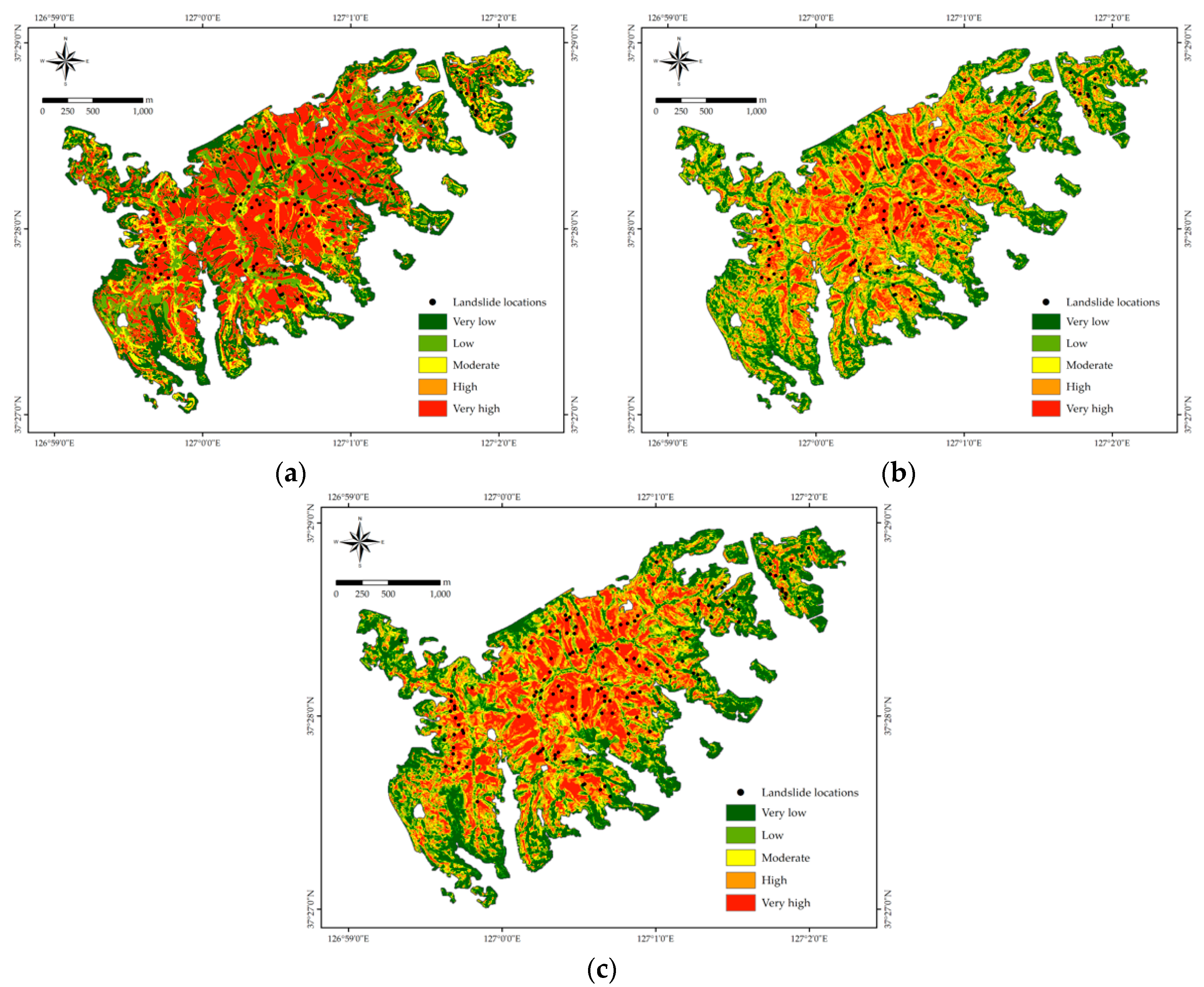
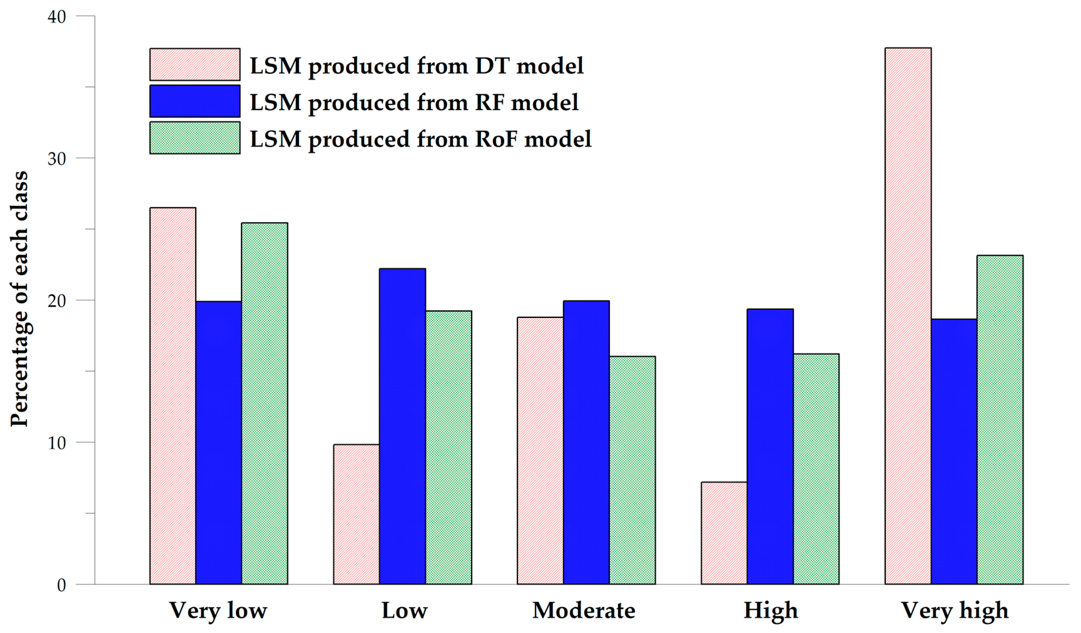
4.2. Landslide Susceptibility Mapping
4.2.1. Decision Trees
4.2.2. Random Forest
4.2.3. Rotation Forest
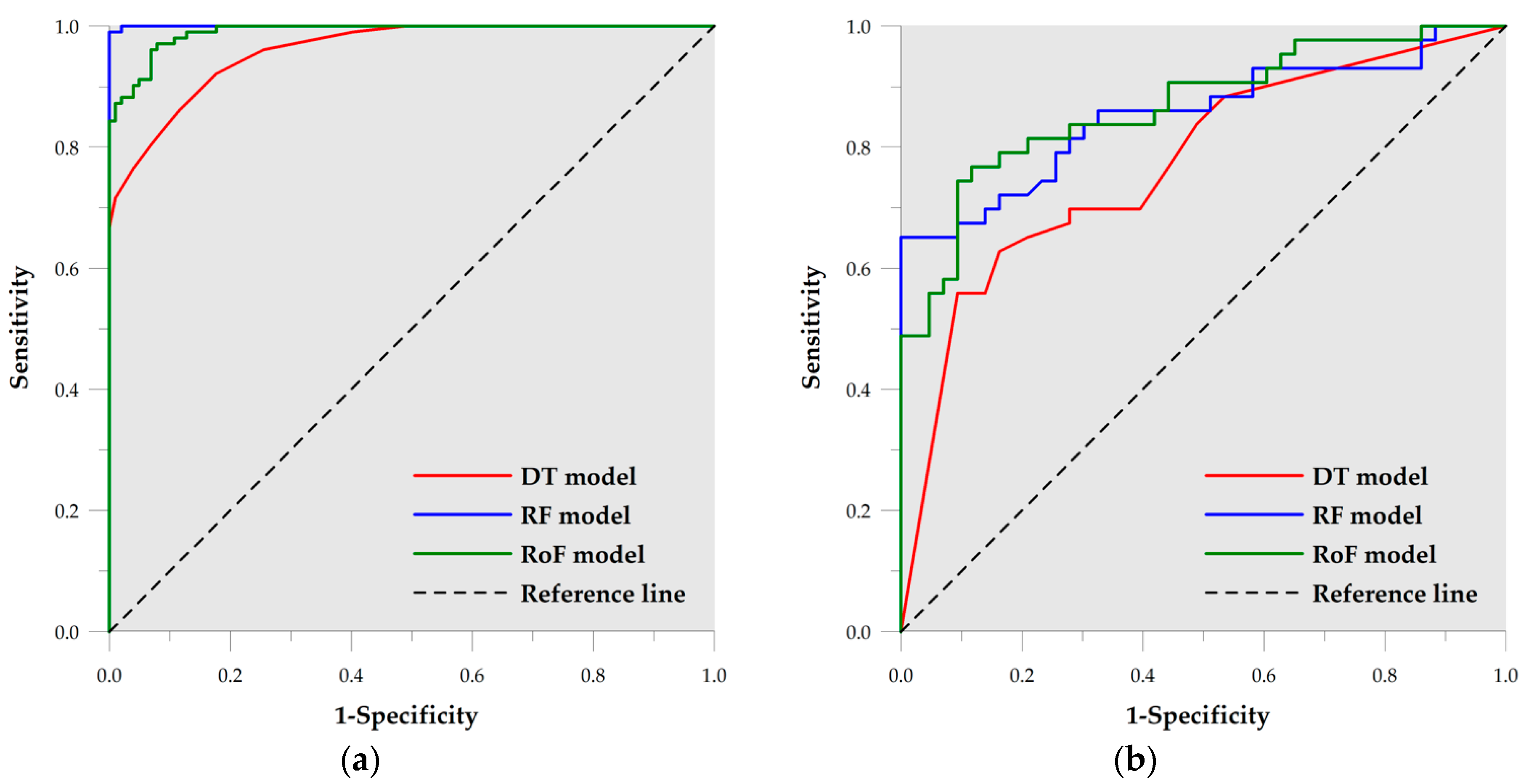
4.3. Model Validation and Comparison
4.3.1. Statistical Indices
4.3.2. Receiver Operating Characteristic Curve
5. Discussion
6. Conclusions
Author Contributions
Acknowledgments
Conflicts of Interest
Appendix A

References
- Brabb, E.E. Innovative Approaches to Landslide Hazard Mapping. In Proceedings of the 4th International Symposium on Landslides, Toronto, ON, Canada, 16–21 September 1984; USGS: Reston, VA, USA, 1985; pp. 307–324. [Google Scholar]
- Guzzetti, F.; Carrara, A.; Cardinali, M.; Reichenbach, P.; Galli, M.; Ardizzone, F. Landslide Hazard Evaluation: An Aid to a Sustainable Development. Geomorphology 1999, 31, 181–216. [Google Scholar] [CrossRef]
- Sahin, E.K.; Colkesen, I.; Kavzoglu, T. A Comparative Assessment of Canonical Correlation Forest, Random Forest, Rotation Forest and Logistic Regression Methods for Landslide Susceptibility Mapping. Geocarto Int. 2018, 1–23. [Google Scholar] [CrossRef]
- Pham, B.T.; Shirzadi, A.; Bui, D.T.; Prakash, I.; Dholakia, M.B. A Hybrid Machine Learning Ensemble Approach Based on a Radial Basis Function Neural Network and Rotation Forest for Landslide Susceptibility Modeling: A Case Study in the Himalayan Area, India. Int. J. Sediment. Res. 2018, 33, 157–170. [Google Scholar] [CrossRef]
- Yilmaz, I. Comparison of Landslide Susceptibility Mapping Methodologies for Koyulhisar, Turkey: Conditional Probability, Logistic Regression, Artificial Neural Networks, and Support Vector Machine. Environ. Earth Sci. 2010, 61, 821–836. [Google Scholar] [CrossRef]
- Yalcin, A.; Reis, S.; Aydinoglu, A.C.; Yomralioglu, T. A GIS-Based Comparative Study of Frequency Ratio, Analytical Hierarchy Process, Bivariate Statistics and Logistics Regression Methods for Landslide Susceptibility Mapping in Trabzon, NE Turkey. Catena 2011, 85, 274–287. [Google Scholar] [CrossRef]
- Mohammady, M.; Pourghasemi, H.R.; Pradhan, B. Landslide Susceptibility Mapping at Golestan Province, Iran: A Comparison between Frequency Ratio, Dempster–Shafer, and Weights-Of-Evidence Models. J. Asian Earth Sci. 2012, 61, 221–236. [Google Scholar] [CrossRef]
- Park, S.; Choi, C.; Kim, B.; Kim, J. Landslide Susceptibility Mapping Using Frequency Ratio, Analytic Hierarchy Process, Logistic Regression, and Artificial Neural Network Methods at the Inje Area, Korea. Environ. Earth Sci. 2013, 68, 1443–1464. [Google Scholar] [CrossRef]
- Pham, B.T.; Pradhan, B.; Bui, D.T.; Prakash, I.; Dholakia, M.B. A comparative study of different machine learning methods for landslide susceptibility assessment: A case study of Uttarakhand area (India). Environ. Modell. Softw. 2016, 84, 240–250. [Google Scholar] [CrossRef]
- Naghibi, S.A.; Pourghasemi, H.R.; Dixon, B. GIS-Based Groundwater Potential Mapping Using Boosted Regression Tree, Classification and Regression Tree, and Random Forest Machine Learning Models in Iran. Environ. Monit. Assess. 2016, 188, 44. [Google Scholar] [CrossRef]
- Pourghasemi, H.R.; Rahmati, O. Prediction of the Landslide Susceptibility: Which Algorithm, Which Precision. Catena 2018, 162, 177–192. [Google Scholar] [CrossRef]
- Bui, D.T.; Pradhan, B.; Lofman, O.; Revhaug, I.; Dick, O.B. Landslide Susceptibility Mapping at Hoa Binh Province (Vietnam) Using an Adaptive Neuro–Fuzzy Inference System and GIS. Comput. Geosci. 2012, 45, 199–211. [Google Scholar] [CrossRef]
- Conforti, M.; Pascale, S.; Robustelli, G.; Sdao, F. Evaluation of Prediction Capability of the Artificial Neural Networks for Mapping Landslide Susceptibility in the Turbolo River Catchment (Northern Calabria, Italy). Catena 2014, 113, 236–250. [Google Scholar] [CrossRef]
- Kawabata, D.; Bandibas, J. Landslide Susceptibility Mapping Using Geological Data, a DEM from ASTER Images and an Artificial Neural Network (ANN). Geomorphology 2009, 113, 97–109. [Google Scholar] [CrossRef]
- Pourghasemi, H.R.; Pradhan, B.; Gokceoglu, C. Application of Fuzzy Logic and Analytical Hierarchy Process (AHP) to Landslide Susceptibility Mapping at Haraz Watershed, Iran. Nat. Hazards 2012, 63, 965–996. [Google Scholar] [CrossRef]
- Zhu, A.X.; Wang, R.; Qiao, J.; Qin, C.Z.; Chen, Y.; Liu, J.; Zhu, T. An Expert Knowledge-Based Approach to Landslide Susceptibility Mapping Using GIS and Fuzzy Logic. Geomorphology 2014, 214, 128–138. [Google Scholar] [CrossRef]
- Pradhan, B. A Comparative Study on the Predictive Ability of the Decision Tree, Support Vector Machine and Neuro-Fuzzy Models in Landslide Susceptibility Mapping Using GIS. Comput. Geosci. 2013, 51, 350–365. [Google Scholar] [CrossRef]
- Bui, D.T.; Pradhan, B.; Lofman, O.; Revhaug, I. Landslide Susceptibility Assessment in Vietnam Using Support Vector Machines, Decision Tree, and Naive Bayes Models. Math. Probl. Eng. 2012, 2012, 26. [Google Scholar] [CrossRef]
- Lee, S.; Hong, S.M.; Jung, H.S. A Support Vector Machine for Landslide Susceptibility Mapping in Gangwon Province, Korea. Sustainability 2017, 9, 48. [Google Scholar] [CrossRef]
- Youssef, A.M.; Pourghasemi, H.R.; Pourtaghi, Z.S.; Al-Katheeri, M.M. Landslide Susceptibility Mapping Using Random Forest, Boosted Regression Tree, Classification and Regression Tree, and General Linear Models and Comparison of Their Performance at Wadi Tayyah Basin, Asir Region, Saudi Arabia. Landslides 2016, 13, 839–856. [Google Scholar] [CrossRef]
- Chen, W.; Zhang, S.; Li, R.; Shahabi, H. Performance Evaluation of the GIS–Based Data Mining Techniques of Best-First Decision Tree, Random Forest, and Naive Bayes Tree for Landslide Susceptibility Modeling. Sci. Total Environ. 2018, 644, 1006–1018. [Google Scholar] [CrossRef]
- Kadavi, P.; Lee, C.W.; Lee, S. Application of ensemble–based machine learning models to landslide susceptibility mapping. Remote Sens. 2018, 10, 1252. [Google Scholar] [CrossRef]
- Nguyen, Q.K.; Tien Bui, D.; Hoang, N.D.; Trinh, P.; Nguyen, V.H.; Yilmaz, I. A Novel Hybrid Approach Based on Instance Based Learning Classifier and Rotation Forest Ensemble for Spatial Prediction of Rainfall-Induced Shallow Landslides Using GIS. Sustainability 2017, 9, 813. [Google Scholar] [CrossRef]
- Rodriguez, J.J.; Kuncheva, L.I.; Alonso, C.J. Rotation Forest: A New Classifier Ensemble Method. IEEE Trans. Pattern Anal. 2006, 28, 1619–1630. [Google Scholar] [CrossRef] [PubMed]
- Liu, K.H.; Huang, D.S. Cancer Classification Using Rotation Forest. Comput. Biol. Med. 2008, 38, 601–610. [Google Scholar] [CrossRef]
- De Bock, K.W.; Van Den Poel, D. An Empirical Evaluation of Rotation-Based Ensemble Classifiers for Customer Churn Prediction. Expert Syst. Appl. 2011, 38, 12293–12301. [Google Scholar] [CrossRef]
- Nanni, L.; Lumini, A. An Experimental Comparison of Ensemble of Classifiers for Bankruptcy Prediction and Credit Scoring. Expert Syst. Appl. 2009, 36, 3028–3033. [Google Scholar] [CrossRef]
- Choudhury, S.D.; Tjahjadi, T. Clothing and Carrying Condition Invariant Gait Recognition Based on Rotation Forest. Pattern Recog. Lett. 2016, 80, 1–7. [Google Scholar] [CrossRef]
- Du, P.; Samat, A.; Waske, B.; Liu, S.; Li, Z. Random Forest and Rotation Forest for Fully Polarized SAR Image Classification Using Polarimetric and Spatial Features. ISPRS J. Photogramm. 2015, 105, 38–53. [Google Scholar] [CrossRef]
- Xia, J.; Du, P.; He, X.; Chanussot, J. Hyperspectral Remote Sensing Image Classification Based on Rotation Forest. Geosci. Remote. Sens. Lett. 2016, 11, 239–243. [Google Scholar] [CrossRef]
- Korean Geotechnical Society (KGS). The Study on Investigation of Cause and Development of Restoration Policy about Landslide in Wumyon Area; Korean Geotechnical Society: Seoul, Korea, 2011. (In Korean) [Google Scholar]
- Park, S.; Kim, J. Landslide Susceptibility Mapping Based on Random Forest and Boosted Regression Tree Models, and a Comparison of Their Performance. Appl. Sci. 2019, 9, 942. [Google Scholar] [CrossRef]
- Park, D.W.; Nikhil, N.V.; Lee, S.R. Landslide and Debris Flow Susceptibility Zonation using TRIGRS for the 2011 Seoul Landslide Event. Nat. Hazards Earth Syst. Sci. 2013, 13, 2833–2849. [Google Scholar] [CrossRef]
- Weiss, A. Topographic Position and Landforms Analysis. In Proceedings of the Poster Presentation, ESRI User Conference, San Diego, CA, USA, 9–13 July 2001; The Nature Conservoncy: Arlington County, VA, USA, 2001; p. 200. [Google Scholar]
- Pike, R.J.; Wilson, S.E. Elevation-Relief Ratio, Hypsometric Integraland Geomorphic Area—Altitude Analysis. Geol. Soc. Am. Bull. 1971, 82, 1079–1084. [Google Scholar] [CrossRef]
- Beven, K.J.; Kirkby, M.J. A Physically Based, Variable Contributing Area Model of Basin Hydrology/Un Modele a Base Physique De Zone Dappel Variable de Lhydrologie Du Bassin Versant. Hydrol. Sci. J. 1979, 24, 43–69. [Google Scholar] [CrossRef]
- Moore, I.D.; Grayson, R.B.; Ladson, A.R. Digital Terrain Modelling: A Review of Hydrological, Geomorphological, and Biological Applications. Hydrol. Process. 1991, 5, 3–30. [Google Scholar] [CrossRef]
- Kira, K.; Rendell, L.A. Practical Approach to Feature Selection. In Proceedings of the 9th International Conference on Machine Learning, Aberdeen, Scotland, UK, 1–3 July 1992; ICML: Aberdeen, Scotland, UK, 1992; pp. 249–256. [Google Scholar]
- Kononenko, I. Estimating Attributes: Analysis and Extensions of RELIEF. In Proceedings of the European Conference on Machine Learning, Berlin, Germany, 6–8 April 1994; Springer Science Business Media: Berlin, Germany, 1994; pp. 171–182. [Google Scholar]
- Robnik-Sikonja, M.; Kononenko, I. An Adaptation of Relief for Attribute Estimation in Regression. In Proceedings of the 14th International Conference on Machine Learning, Nashville, TN, USA, 8–12 July 1997; IEEE: Nashville, TN, USA, 1997; Volume 5, pp. 296–304. [Google Scholar]
- Kass, G.V. An Exploratory Technique for Investigating Large Quantities of Categorical Data. Appl. Stat. 1980, 29, 119–127. [Google Scholar] [CrossRef]
- Breiman, L.; Friedman, J.H.; Olshen, R.A.; Stone, C.J. Classification and Regression Trees; Chapman & Hall: London, UK, 1984. [Google Scholar]
- Quinlan, J.R. Induction of Decision Trees. Mach. Learn. 1986, 1, 81–106. [Google Scholar] [CrossRef]
- Quinlan, J.R. C4.5: Programs for Machine Learning; Morgan Kaufmann Publishers: Burlington, NJ, USA, 1993. [Google Scholar]
- Breiman, L. Random Forests. Mach. Learn. 2001, 45, 5–32. [Google Scholar] [CrossRef]
- Micheletti, N.; Foresti, L.; Robert, S.; Leuenberger, M.; Pedrazzini, A.; Jaboyedoff, M.; Kanevski, M. Machine Learning Feature Selection Methods for Landslide Susceptibility Mapping. Math. Geosci. 2014, 46, 33–57. [Google Scholar] [CrossRef]
- Arabameri, A.; Pradhan, B.; Pourghasemi, H.; Rezaei, K.; Kerle, N. Spatial Modelling of Gully Erosion Using GIS and R Programing: A Comparison among Three Data Mining Algorithms. Appl. Sci. 2018, 8, 1369. [Google Scholar] [CrossRef]
- Witten, I.H.; Frank, E.; Mark, A.H. Data Mining: Practical Machine Learning Tools and Techniques, 3rd ed.; Morgan Kaufmann Publishers: Burlington, NJ, USA, 2011. [Google Scholar]
- Shirzadi, A.; Soliamani, K.; Habibnejhad, M.; Kavian, A.; Chapi, K.; Shahabi, H.; Ahmad, A. Novel GIS Based Machine Learning Algorithms for Shallow Landslide Susceptibility Mapping. Sensors 2018, 18, 3777. [Google Scholar] [CrossRef]
- Dou, J.; Yunus, A.P.; Bui, D.T.; Merghadi, A.; Sahana, M.; Zhu, Z.; Pham, B.T. Assessment of Advanced Random Forest and Decision Tree Algorithms for Modeling Rainfall-Induced Landslide Susceptibility in the Izu-Oshima Volcanic Island, Japan. Sci. Total Environ. 2019, 662, 332–346. [Google Scholar] [CrossRef] [PubMed]
- Garosi, Y.; Sheklabadi, M.; Conoscenti, C.; Pourghasemi, H.R.; Van Oost, K. Assessing the Performance of GIS-Based Machine Learning Models with Different Accuracy Measures for Determining Susceptibility to Gully Erosion. Sci. Total Environ. 2019, 664, 1117–1132. [Google Scholar] [CrossRef] [PubMed]
- Landis, J.R.; Koch, G.G. The Measurement of Observer Agreement for Categorical Data. Biometrics 1977, 33, 159–174. [Google Scholar] [CrossRef] [PubMed]
- Tehrany, M.S.; Pradhan, B.; Jebur, M.N. Spatial Prediction of Flood Susceptible Areas Using Rule Based Decision Tree (DT) and a Novel Ensemble Bivariate and Multivariate Statistical Models in GIS. J. Hydrol. 2013, 504, 69–79. [Google Scholar] [CrossRef]
- Elith, J.; Leathwick, J.R.; Hastie, T.A. Working Guide to Boosted Regression Trees. J. Anim. Ecol. 2008, 77, 802–813. [Google Scholar] [CrossRef] [PubMed]
- Kuncheva, L.I. Combining Pattern Classifiers: Methods and Algorithms; JohnWiley & Sons, Inc.: Hoboken, NJ, USA, 2004; pp. 203–234. [Google Scholar]
- Kavzoglu, T.; Colkesen, I. An Assessment of the Effectiveness of a Rotation Forest Ensemble for Land-Use and Land-Cover Mapping. Int. J. Remote Sens. 2013, 34, 4224–4241. [Google Scholar] [CrossRef]


| Factor | Class | Number of Pixels in Domain | Number of Landslide Pixels | Frequency Ratio | Normalized Class |
|---|---|---|---|---|---|
| Altitude | 20.00–65.56 | 49,073 | 8 | 0.427 | 1 |
| 65.56–95.17 | 68,099 | 18 | 0.692 | 2 | |
| 95.17–125.92 | 54,415 | 20 | 0.962 | 3 | |
| 125.92–158.95 | 40,131 | 23 | 1.5 | 6 | |
| 158.95–195.40 | 26,637 | 12 | 1.179 | 4 | |
| 195.40–236.40 | 17,935 | 16 | 2.336 | 7 | |
| >236.40 | 10,757 | 5 | 1.217 | 5 | |
| Slope | 0.0 –7.10 | 12,845 | 1 | 0.204 | 1 |
| 7.10–13.38 | 44,632 | 6 | 0.352 | 2 | |
| 13.38–18.29 | 68,462 | 26 | 0.994 | 4 | |
| 18.29–22.94 | 64,308 | 26 | 1.059 | 5 | |
| 22.94–27.85 | 46,338 | 28 | 1.582 | 7 | |
| 27.85–34.13 | 24,538 | 14 | 1.494 | 6 | |
| >34.13 | 5924 | 1 | 0.442 | 3 | |
| Aspect | Flat | 2124 | 0 | 0 | 1 |
| North | 33,682 | 12 | 0.933 | 5 | |
| Northeast | 32,212 | 7 | 0.569 | 2 | |
| East | 36,219 | 8 | 0.578 | 3 | |
| Southeast | 34,795 | 17 | 1.279 | 7 | |
| South | 37,218 | 16 | 1.126 | 6 | |
| Southwest | 35,630 | 19 | 1.396 | 8 | |
| West | 25,446 | 14 | 1.44 | 9 | |
| Northwest | 29,721 | 9 | 0.793 | 4 | |
| Profile | Concave | 131,376 | 62 | 1.236 | 3 |
| curvature | Flat | 3774 | 1 | 0.694 | 1 |
| Convex | 131,897 | 39 | 0.774 | 2 | |
| Plan curvature | Concave | 124,461 | 57 | 1.199 | 3 |
| Flat | 6489 | 1 | 0.403 | 1 | |
| Convex | 136,097 | 44 | 0.846 | 2 | |
| Terrain position | −8.87–-1.82 | 7749 | 6 | 2.027 | 7 |
| index | −1.82–-0.78 | 35,071 | 18 | 1.344 | 6 |
| −0.78–-0.14 | 65,552 | 31 | 1.238 | 5 | |
| −0.14–0.50 | 80,859 | 31 | 1.004 | 4 | |
| 0.50–1.30 | 47,450 | 10 | 0.552 | 2 | |
| 1.30–2.50 | 24,331 | 6 | 0.646 | 3 | |
| >2.50 | 6035 | 0 | 0 | 1 | |
| Elevation-relief | 0.01–0.33 | 9143 | 0 | 0 | 1 |
| ratio | 0.33–0.42 | 26,087 | 1 | 0.1 | 2 |
| 0.42–0.48 | 52,853 | 25 | 1.238 | 5 | |
| 0.48–0.52 | 72,581 | 30 | 1.082 | 4 | |
| 0.52–0.58 | 60,144 | 33 | 1.437 | 7 | |
| Elevation-relief | 0.58–0.67 | 32,250 | 6 | 0.487 | 3 |
| ratio | >0.67 | 13,989 | 7 | 1.31 | 6 |
| Slope length and | 0.00–4.83 | 63,353 | 10 | 0.413 | 2 |
| slope steepness | 4.83–12.55 | 106,388 | 37 | 0.911 | 3 |
| 12.55–21.24 | 69,171 | 36 | 1.363 | 4 | |
| 21.24–34.75 | 22,367 | 15 | 1.756 | 5 | |
| 34.75–56.96 | 4185 | 3 | 1.877 | 6 | |
| 56.96–96.64 | 1376 | 1 | 1.903 | 7 | |
| >93.64 | 207 | 0 | 0 | 1 | |
| Topographic | −7.57–-4.79 | 24,064 | 3 | 0.326 | 1 |
| wetness index | −4.79–-1.25 | 4072 | 1 | 0.643 | 3 |
| −1.25–2.01 | 49,146 | 14 | 0.746 | 4 | |
| 2.01–3.35 | 92,435 | 42 | 1.19 | 6 | |
| 3.35–4.79 | 70,461 | 33 | 1.226 | 7 | |
| 4.79–7.28 | 21,767 | 8 | 0.962 | 5 | |
| >7.28 | 5102 | 1 | 0.513 | 2 | |
| Stream power | −13.82–-11.17 | 1402 | 1 | 1.867 | 7 |
| index | −11.17–-8.61 | 7285 | 0 | 0 | 1 |
| −8.61–-4.47 | 21,359 | 3 | 0.368 | 2 | |
| −4.47–-0.15 | 46,837 | 7 | 0.391 | 3 | |
| −0.15–1.27 | 91,085 | 41 | 1.178 | 5 | |
| 1.27–3.12 | 87,844 | 45 | 1.341 | 6 | |
| >3.12 | 11,235 | 5 | 1.165 | 4 | |
| Timber type | Pine | 858 | 0 | 0 | 3 |
| Nut pine | 9578 | 2 | 0.547 | 5 | |
| Larch | 5577 | 2 | 0.939 | 7 | |
| Pitch pine | 1724 | 0 | 0 | 2 | |
| Sawtooth oak | 46,898 | 14 | 0.782 | 6 | |
| Mongolian oak | 4739 | 0 | 0 | 1 | |
| Oriental oak | 2244 | 1 | 1.167 | 10 | |
| Other oak | 104,176 | 41 | 1.03 | 8 | |
| Popular | 5643 | 5 | 2.32 | 12 | |
| False acasia | 63,896 | 28 | 1.147 | 9 | |
| Other broadleaf | 15,027 | 8 | 1.394 | 11 | |
| Mixed forest | 6687 | 1 | 0.392 | 4 | |
| Timber diameter | 6–18cm | 8677 | 2 | 0.603 | 1 |
| 18–30cm | 258,370 | 100 | 1.013 | 2 | |
| Timber age | 21–30ages | 6203 | 1 | 0.422 | 2 |
| 31–40ages | 251,913 | 100 | 1.039 | 3 | |
| 41–50ages | 8931 | 1 | 0.293 | 1 | |
| Timber density | 51–70% | 11,930 | 3 | 0.658 | 1 |
| >70% | 255,117 | 99 | 1.016 | 2 |
| No | Conditioning Factor | Importance |
|---|---|---|
| 1 | Elevation-relief ratio | 0.182 |
| 2 | Aspect | 0.158 |
| 3 | Altitude | 0.157 |
| 4 | Slope | 0.148 |
| 5 | Timber type | 0.107 |
| 6 | Topographic wetness index | 0.102 |
| 7 | Slope length | 0.101 |
| 8 | Topographic position index | 0.100 |
| 9 | Stream power index | 0.078 |
| 10 | Plan curvature | 0.058 |
| 11 | Profile curvature | 0.009 |
| 12 | Timber diameter | 0.000 |
| 13 | Timber age | 0.000 |
| 14 | Timber density | 0.000 |
| Calibration Dataset | Validation Dataset | |||||
|---|---|---|---|---|---|---|
| DT | RF | RoF | DT | RF | RoF | |
| Sensitivity | 0.880 | 1.000 | 0.957 | 0.707 | 0.833 | 0.882 |
| Specificity | 0.865 | 0.962 | 0.891 | 0.689 | 0.740 | 0.750 |
| Precision | 0.863 | 0.961 | 0.828 | 0.674 | 0.698 | 0.698 |
| Accuracy | 0.873 | 0.980 | 0.922 | 0.698 | 0.779 | 0.802 |
| Kappa | 0.745 | 0.961 | 0.843 | 0.395 | 0.558 | 0.605 |
| AUROC | Std. Error | Asymptotic Sig. | Asymptotic 95% Confidence Interval | ||
|---|---|---|---|---|---|
| Lower Bound | Upper Bound | ||||
| DT | 0.960 | 0.011 | 0.000 | 0.938 | 0.982 |
| RF | 1.000 | 0.000 | 0.000 | 0.999 | 1.000 |
| RoF | 0.990 | 0.004 | 0.000 | 0.982 | 0.998 |
| AUROC | Std. Error | Asymptotic Sig. | Asymptotic 95% Confidence Interval | ||
|---|---|---|---|---|---|
| Lower Bound | Upper Bound | ||||
| DT | 0.772 | 0.051 | 0.000 | 0.672 | 0.872 |
| RF | 0.853 | 0.043 | 0.000 | 0.770 | 0.937 |
| RoF | 0.868 | 0.039 | 0.000 | 0.792 | 0.944 |
© 2019 by the authors. Licensee MDPI, Basel, Switzerland. This article is an open access article distributed under the terms and conditions of the Creative Commons Attribution (CC BY) license (http://creativecommons.org/licenses/by/4.0/).
Share and Cite
Park, S.; Hamm, S.-Y.; Kim, J. Performance Evaluation of the GIS-Based Data-Mining Techniques Decision Tree, Random Forest, and Rotation Forest for Landslide Susceptibility Modeling. Sustainability 2019, 11, 5659. https://doi.org/10.3390/su11205659
Park S, Hamm S-Y, Kim J. Performance Evaluation of the GIS-Based Data-Mining Techniques Decision Tree, Random Forest, and Rotation Forest for Landslide Susceptibility Modeling. Sustainability. 2019; 11(20):5659. https://doi.org/10.3390/su11205659
Chicago/Turabian StylePark, Soyoung, Se-Yeong Hamm, and Jinsoo Kim. 2019. "Performance Evaluation of the GIS-Based Data-Mining Techniques Decision Tree, Random Forest, and Rotation Forest for Landslide Susceptibility Modeling" Sustainability 11, no. 20: 5659. https://doi.org/10.3390/su11205659
APA StylePark, S., Hamm, S.-Y., & Kim, J. (2019). Performance Evaluation of the GIS-Based Data-Mining Techniques Decision Tree, Random Forest, and Rotation Forest for Landslide Susceptibility Modeling. Sustainability, 11(20), 5659. https://doi.org/10.3390/su11205659