Short-Term Wind Power Prediction Based on Improved Chicken Algorithm Optimization Support Vector Machine

Abstract

Renewable energy technologies are essential contributors to sustainable energy including renewable energy sources. Wind energy is one of the important renewable energy resources. Therefore, efficient and consistent utilization of wind energy has been an important issue. The wind speed has the characteristics of intermittence and instability. If the wind power is directly connected to the grid, it will impact the voltage and frequency of the power system. Short-term wind power prediction can reduce the impact of wind power on the power grid and the stability of power system operation is guaranteed. In this study, the improved chicken swarm algorithm optimization support vector machine (ICSO-SVM) model is proposed to predict the wind power. The traditional chicken swarm optimization algorithm (CSO) easily falls into a local optimum when solving high-dimensional problems due to its own characteristics. So the CSO algorithm is improved and the ICSO algorithm is developed. In order to verify the validity of the ICSO-SVM model, the following work has been done. (1) The particle swarm optimization (PSO), ICSO, CSO and differential evolution algorithm (DE) are tested respectively by four standard testing functions, and the results are compared. (2) The ICSO-SVM and CSO-SVM models are tested respectively by two sets of wind power data. This study draws the following conclusions: (1) the PSO, CSO, DE and ICSO algorithms are tested by the four standard test functions and the test data are analyzed. By comparing it with the other three optimization algorithms, the ICSO algorithm has the best convergence effect. (2) The number of training samples has an obvious impact on the prediction results. The average relative error percentage and root mean square error (RMSE) values of the ICSO model are smaller than those of CSO-SVM model. Therefore, the ICSO-SVM model can efficiently provide credible short-term predictions for wind power forecasting.

1. Introduction

The problems of environmental pollution, ecological damage, conventional energy depletion and haze weather have become increasingly serious. Countries around the world attach great importance to the development and utilization of green energy, especially where there is serious environmental pollution. As clean energy power generation technology becomes mature, the proportion of clean energy power generation in the world power supply is increasing year by year. Wind power generation and photovoltaic power generation account for the largest proportion of new energy generation [1,2,3,4]. From 1980 to the 1990s, wind power technology was rapidly developed and gradually matured. Wind power generation has brought great convenience to people due to its advantages of renewable, clean and environmental protection. Wind power installations are commercially available in more than 70 countries around the world, with 22 countries having installed capacity exceeding 1 GW. It is estimated that by 2030, European wind power installations will reach 30 billion watts, which can meet 20% of Europe’s electricity demand. But wind power has its own limitations, and the biggest influence on wind power output is weather changes [5,6,7]. Because of the intermittent characteristics of wind power generation, wind power generation will impact the power grid. If wind power is directly connected to the grid, it will affect the voltage and frequency of the power system, thus affecting the stable operation of the power system [8,9]. By forecasting wind power, the power generation plan can be reasonably arranged, which can avoid large fluctuations in the power system. The support vector machine (SVM) has better robustness, can avoid dimension disaster, and has strong non-linear mapping ability. So this study uses the SVM to predict short-term wind power.

Naik et al. [10] used a new method to predict short-term wind power. This method combines variational mode decomposition (VMD) and low rank multi-kernel ridge regression (MKRR). The parameters of the model are optimized by the mutated firefly algorithm with global optima concept (MFAGO) optimization algorithm. Hong et al. [11] proposed a prediction model to forecast ultra-short-term wind power. In the method, the time series is decomposed into two components by morphological high frequency filter. The double similarity search algorithm is used to predict high frequency component. Finally, each component is predicted by the least-squares support-vector machines (LSSVM). And The final prediction results are synthesized. The wind power was predicted by the support vector machine (SVM), as in [9]. The parameters of SVM are optimized by the enhanced particle swarm optimization algorithm in this method to improve the prediction accuracy. Bhaskar et al. [12] used a feed-forward neural network (FFNN) to predict wind power. Firstly, the wind signal is decomposed by wavelet transform, and each decomposed signal is regressed by adaptive wavelet neural network (AWNN). Then, the non-linear mapping relationship between wind speed and wind output is constructed by FFNN. Wang et al. [13] used the sparse Bayesian-based robust functional regression model to predict wind speed. This method reduces the adverse effects of redundant function variables on prediction results. The robustness of the model is improved by assuming multiple mixture Gaussian priors of prediction errors. Wang et al. [14] used a deep belief network model to predict wind power. In this method, the k-means clustering algorithm was used to deal with the numerical weather prediction data, which can improve the prediction accuracy. Liu et al. [9] used a hybrid support vector machine to predict wind power. This method combines wavelet transform and feature extraction.

Short-term wind power was predicted by using an improved support vector machine method, as in [15]. In the method, invalid data in the original data is first removed. The high-frequency component of the original signal is removed by the wavelet transform. Finally, the support vector machine is used to predict the wind power. The short-term wind power was predicted by the improved random forest model, as in [16]. Firstly, the data is preprocessed to remove the redundant items from the original data, and a new external verification index related to wind speed in numerical weather prediction is proposed. A framework based on the bandwidth selection concept was proposed for new flexible kernel density estimation in [17]. This method uses diffusion-based nuclear density estimator to achieve high-quality interval prediction of non-stationary wind power time series. Zheng et al. [18] presented a comprehensive hybrid method to predict the short-term wind power. Three algorithms are combined in this method.

In this study, the parameters of the SVM are optimized by the improved chicken swarm optimization algorithm (ICSO). Shi et al. [19] introduced two strategies in the chicken swarm algorithm and propose the modified parallel cat swarm optimization (MPCSO) algorithm. The two strategies are monomers turbulence in rooster (MTR) and particle renovation in hen (PRH). It can be found that the MPCSO algorithm is better than other algorithms. Wu et al. [20] used a chaotic sequence to initialize chicken position. This method improves the update strategy of hen position and chicken position. Adaptive inertia weight is added to the hen position updating equation. The following coefficient is added to the chick position updating equation. Through the above improvements, the local search ability and global search ability of the chicken swarm optimization algorithm (CSO) algorithm can be improved. The crossover operation was introduced in ICSO algorithm, as in [21]. After the crossover operation, two new offspring replace the two hens with poor fitness values. This study has made the following improvements to the CSO algorithm. Firstly, the self-learning factor is introduced in the hen position update equation. Secondly, when the fitness values of hen are updated, the flock particles are sorted. Some cock particles with good fitness replace hen particles with poor fitness. Finally, the optimal individual learning part is introduced in the chick position update equation.

2. Wind Power Prediction Model Materials and Methods

2.1. Support Vector Machine (SVM) Regression

SVM is a machine learning method based on statistical learning theory, which belongs to the supervised learning method. The generalization ability of the learning machine is improved by seeking structural risk minimization. Moreover, the minimization of experience risk and confidence range is realized [22,23]. SVM is widely used in forecasting fields due to its high generalization ability, strong non-linear mapping ability and small sample size, such as photovoltaic power prediction, battery life prediction, insulated gate bipolar transistor (IGBT) life prediction and wind power prediction [24,25]. The specific regression principle of SVM is as follows.

Suppose the sample set is $P=\left\{(x_i,y_i),i=1,2,\cdots ,u\right\}$. $x_i\in R^m$ represents the input vector of the ith sample. $y_i\in R$ represents the output vector of the ith sample [26,27]. The regression function is obtained by mapping data to high-dimensional space:

$$B(x)=r\ast z(x)+l$$

(1)

where $r$ is the weight coefficient; $z(\cdot )$ is the mapping function, which maps data to high-dimensional space and regression function is constructed in high-dimensional space; $l$ is the threshold vector.

The problem of upper solution is transformed into the problem of minimizing the target of the following equation:

$$\begin{array}{c}\min \frac{1}{2}{r}^{T}r\\ s.t.\{\begin{array}{c}y-rz(x)-l\le q\\ y-rz(x)-l\ge -q\end{array}\end{array}$$

(2)

where $q$ is the insensitive loss parameter. The smaller the value is, the better the effect of regression is.

The slack variable is introduced to the above equation due to the error between the regression value and the original value:

$$\begin{array}{c}\min \frac{1}{2}{r}^{T}r+C{\displaystyle \sum _{i=1}^u({\beta }_i+{\beta }_i^{*})}\\ \{\begin{array}{l}{y}_i-rz(x_i)-l\le q+{\beta }_i\hfill \\ y_i-rz(x_i)-l\ge -q-{\beta }_i^{*}\hfill \\ {\beta }_i\ge 0,{\beta }_i^{*}\ge 0\hfill \end{array}\end{array}$$

(3)

where ${\beta }_i$ is the slack factor; C is the penalty coefficient. The greater the penalty factor is, the greater the penalty for exceeding the error phase is.

The Lagrangian function is introduced to solve the above minimum value problem.

$$\begin{array}{ll}L=& \frac{1}{2}{r}^{T}r+C{\displaystyle \sum _{i=1}^u({\beta }_i+{\beta }_i^{*})}-{\displaystyle \sum _{i=1}^u{\rho }_i}(q+{\beta }_i-y_i+rz(x_i)+l)-\\ & {\displaystyle \sum _{i=1}^u{\rho }_i^{*}(-q-{\beta }_i-y_i+rz(x_i)+l)}-{\displaystyle \sum _{i=1}^n({\lambda }_i{\beta }_i-{\lambda }_i^{*}{\beta }_i^{*})}\end{array}$$

(4)

where $\rho =[{\rho }_1,{\rho }_2,\cdots ,{\rho }_u]$ is the Lagrange multiplier.

According to the Karush–Kuhn–Tucher (KKT) condition, the above equation is expressed as follows:

$$\begin{array}{l}\min \frac{1}{2}{\displaystyle \sum _{i=1,j=1}^u{\rho }_i{\rho }_j{y}_i{y}_j(x_i·x_j)}-{\displaystyle \sum _{i=1}^u{\rho }_i}\hfill \\ s.t.\{\begin{array}{c}0\le {\rho }_i\le C\\ 0\le {\rho }_j\le C\\ {\displaystyle \sum _{i=1}^u{y}_i{\rho }_i=0}\end{array}\hfill \end{array}$$

(5)

The regression function obtained is as follows:

$$B(x)={\displaystyle \sum _{i=1}^n({\rho }_i-{\rho }_i^{*})T(x_i·x)}+l$$

(6)

where $T(·)$ is the kernel function.

The radial basis kernel function with strong generalization ability is used in this paper and its equation is as follows:

$$T(x_i,x)=\exp (-\frac{{\Vert x_i-x\Vert }^2}{2{\sigma }^2})$$

(7)

If the values of the penalty coefficient C and kernel function parameter are not appropriate, the prediction results will be worse. Therefore, in order to obtain appropriate parameters, the parameters of SVM should be optimized to improve the prediction effect of the model.

2.2. Chicken Swarm Optimization (CSO)

Meng et al. [28] put forward the chicken swarm optimization algorithm (CSO). A new swarm intelligence optimization algorithm is proposed to simulate the hierarchy and foraging behaviour of chickens. The population is divided into several subgroups. Every subgroup contains chicks, hens and cocks. The chicken swarm optimization algorithm obeys the following rules:

(1)

The entire population includes several sub-populations, each of which includes a cock, a number of hens and several chicks.

(2)

The fitness value of each particle in the population is calculated. The particles are classified based on the fitness values. A few particles with good fitness values are selected as cocks, a few particles with poor fitness values are selected as chickens, and the rest of the particles are selected as hens.

(3)

Under a certain hierarchy, the dominance relationship and mother child relationship remain unchanged. However, as the chicks grow, the population relationship will change. The hierarchy, dominance relationship, and maternal relationship of the chicken swarm will change once every G time.

(4)

The cock dominates the flock, the hens follow the cock in their own population, and the chicks feed around the hen. Hens randomly join a subpopulation. The relationship between mother and child in the flock is randomly established. The cock with the largest foraging range and the best foraging ability is dominant in the flock. The chick particles have the worst foraging ability and the smallest foraging range. The foraging ability and foraging range of hen particles are between cock particles and chick particles.

In CSO, there are N particles in the whole chicken flock. The number of roosters is defined as N_r. The number of hens is defined as N_h, and the number of chicks is N_c. Different kinds of chickens have different location updating equations when they are finding food [29,30]. Roosters are the most adaptable individuals in chickens and also the most likely to find food in the whole population.

The equation of the position update of cock particles is shown in Equation (8):

$$\begin{array}{l}{P}_i^j(t+1)=P_i^j(t)\ast (1+Randn(0,{\sigma }^2))\\ {\sigma }^2=\{\begin{array}{cc}1& W_i<W_k\\ \exp (\frac{(W_k-W_i)}{\left|W_i\right|+\epsilon })& \mathrm{others}\end{array}\end{array}$$

(8)

where the $k\in [1,c_n]$, and $k\ne i$. $Randn(0,{\sigma }^2)$ is the gauss distribution with the mean value of 0 and the standard deviation of ${\sigma }^2$. The individual position of $P_i^j(t)$ is the value of the jth dimension of the ith individual at the tth iteration. $\epsilon$ is any small constant; k is an arbitrary cock in all cocks except the ith cock; $W_i$ is the fitness value corresponding to the ith cock; $W_k$ is the fitness value corresponding to the kth cock. Hens are the largest proportion of individuals in the whole chicken population. And its location update formula is shown in formula 9.

$$\begin{array}{l}\begin{array}{ll}{P}_i^j(t+1)=& P_i^j(t)+K_1\ast Random\ast (P_{r1}^j(t)-P_i^j(t))\\ & +K_2\ast Random\ast (P_{r2}^j(t)-P_i^j(t))\end{array}\\ K_1=\frac{\exp (W_i-W_{r_1})}{\left|W_i\right|+\epsilon }\\ K_2=\exp (W_{r_2}-W_i)\end{array}$$

(9)

where $Random$ is a random number between 0 and 1, which obeys the standard normal distribution. r₁ means the cock in the group where the ith hen is located. r₂ represents any cock except the cock in the group of the ith hen. So r₁ is different from r₂. The chick follows the hens’ foraging and the chick’s position update formula is shown in formula 10.

$$P_i^j(t+1)=P_i^j(t)+FL\ast [P_m^j(t)-P_i^j(t)]$$

(10)

where $FL$ is the average number of evenly distributed in [0, 2]. $P_m^j(t)$ is the hen position corresponding to the ith chick.

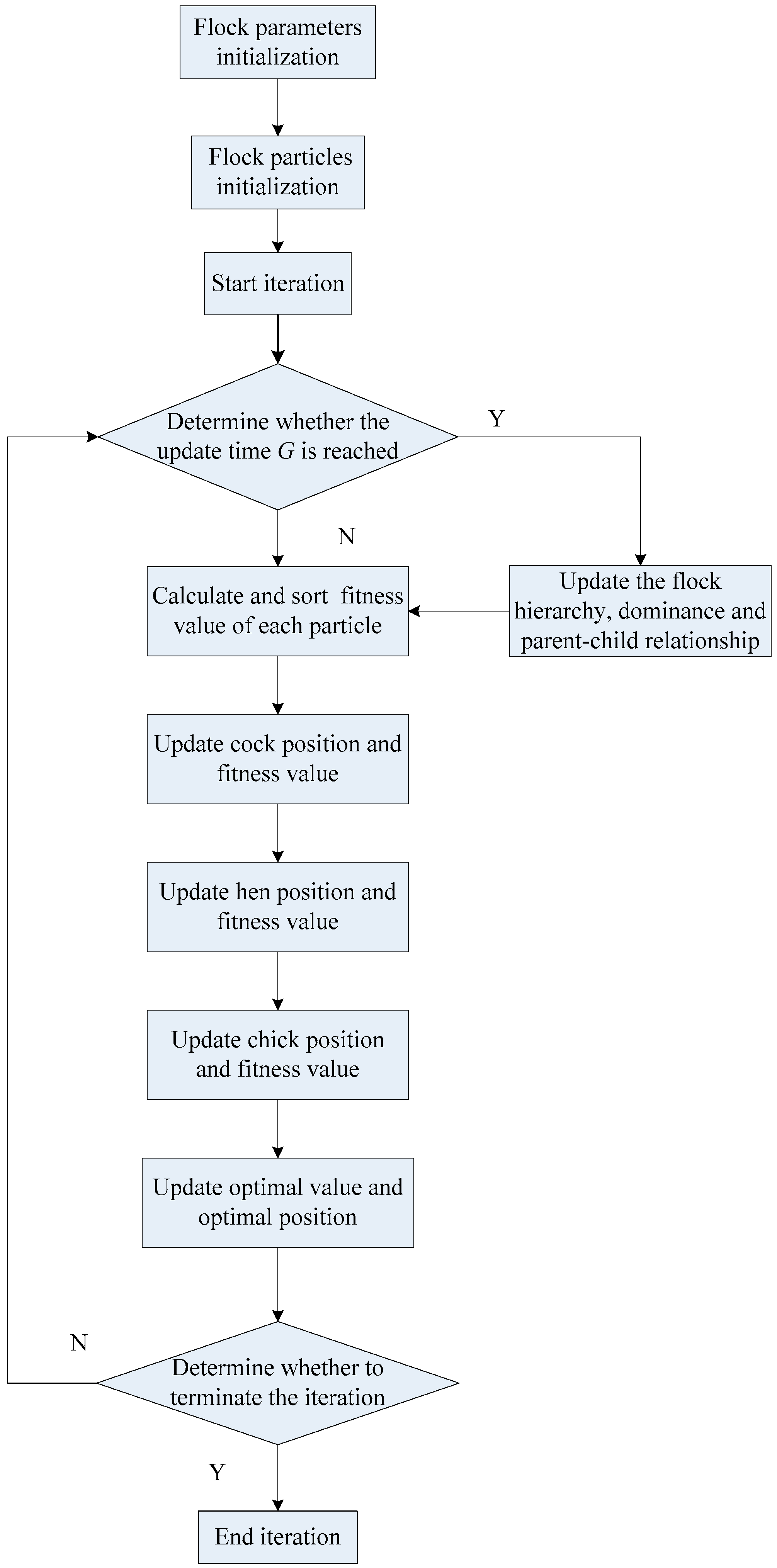
2.3. Improved Chicken Swarm Optimization (ICSO)

In the flock, because the chicks have the worst foraging ability, the smallest foraging range. So the chicks have the worst global search ability. The traditional CSO is prone to premature convergence when solving high-dimensional problems, the improved chicken swarm optimization (ICSO) is introduced in this study. In the traditional CSO algorithm, the number of hens is the largest. Therefore, the search ability of hen particles affects the convergence of CSO algorithm. In Equation (9), hen particles can learn from cock particles in their own population and can learn from cock particles in other populations. However, hen particles have no self-learning ability. In the later stage of convergence, the search range of the whole population decreases. The cock particles tend to fall into the local optimum, which results in the hen particles falling into the local optimum and affects the convergence effect of the whole algorithm.

In this study, the position update equation of hen particles is improved, and a self-learning factor is introduced in the equation. It can be found from Equation (11) that the value of the learning factor is large at the beginning of the iteration, and the hen particles have better global search ability. As the number of iterations increases, the value of learning factor decreases gradually, and the hen particles have better local search ability. The convergence performance of CSO algorithm is also enhanced by improving the local and global search ability of hen particles.

$$w(t)=w_{\max }-\exp {(\frac{M-t}{M})}^3\ast (w_{\max }-w_{\min })$$

(11)

where t is current iterations; M is maximum iterations; w_max = 0.9, w_min = 0.4. The improved hen position update formula is shown in Equation (12):

$$\begin{array}{ll}{P}_i^j(t+1)=& w(t)\ast P_i^j(t)+H_1\ast Random\ast (P_{r1}^j(t)-P_i^j(t))\\ & +H_2\ast Random\ast (P_{r2}^j(t)-P_i^j(t))\end{array}$$

(12)

It can be seen from Equation (12) that the hen particles cannot learn from the cock particles with good fitness value, and can learn by themselves. The improved hen particles have a more flexible foraging strategy than the hen particles before the improvement. When the hen leading the chick falls into the local optimum, the chick can only learn from the following hen, so it will fall into the local optimum, eventually leading to the whole algorithm into the local optimum. The fitness values of hens are calculated and the hen particles are sorted according to the fitness values. The hen particles with poor fitness values are replaced with 80% of the cock particles to ensure the competitiveness of the population. By replacing hen particles with poor fitness values by cock particles with good fitness values, the superiority of hen particles can be guaranteed and the global search ability of chicken flocks can be strengthened.

From Equation (10), it can be found that chicken particles can only learn from hen particles, and the foraging strategy is single. In this regard, the update equation for chicks is improved in two aspects. Firstly, the part of learning from the global optimum individual is added to the chicken position update equation. By learning from the best particles in the chicken flock, the ability of chick particles to jump out of the local optimum can be enhanced. Secondly, At the later stage of the iteration, the population is simplified. In order to increase the diversity of population particles, chick particles are mutated in the late iteration period.

The position update equation of improved chick position is shown in Equation (13).

$$\begin{array}{ll}{P}_i^j(t+1)=P_i^j(t)+FL \ast & [P_m^j(t)-P_i^j(t)]+H\ast [P_{best}^j(t)-P_i^j(t)]\\ & H=\exp (W_{best}-W_i)\end{array}$$

(13)

where the $P_{best}^j(t)$ is optimal individual of chicken swarm; $W_{best}$ is fitness value of the $P_{best}^j(t)$.

The process of improved chicken swarm algorithm is as follows.

(1)

The parameters of the flock are initialized, such as the maximum iterations M, the number of cocks r_n, hens h_n and chicks c_n, update time G and other parameters.

(2)

Initialize chicken particles. The fitness value of each particle is calculated. The fitness values are sorted to find the local optimum and global optimum.

(3)

Start iteration. Determine whether the update time G is reached. If the update time is reached, the flock hierarchy, dominance relationship and parent-child relationship are updated; if the update time is not reached, the positions of the cocks, hens and chicks are calculated according to Equations (9), (12) and (13). The fitness value of each particle is calculated.

(4)

The optimal individual and the location of the optimal individual are updated.

(5)

Determine whether to terminate the procedure. If the closure condition is met, the result is output. If the termination condition is not reached, the program continues to run.

The flow chart of ICSO is shown in Figure 1.

This study uses four standard test functions to test the convergence accuracy of ICSO, CSO, differential evolution algorithm (DE), and particle swarm optimization (PSO) algorithms. Four optimization algorithms are tested 10 times for each test function in 20 and 80 dimensions respectively.

The calculation equation, the value range and the optimal value of the test function are presented in

Table 1. Test function.

Function	Range	Optimum
$f_1={\displaystyle \sum _{i=1}^d{x}_i^2}$	[−100, 100]	0
$f_2={\displaystyle \prod _{i=1}^d\left|x_i\right|}+{\displaystyle \sum _{i=1}^d\left|x_i\right|}$	[−10, 10]	0
$f_3={\displaystyle \sum _{i=1}^d(x_i^2-10\cos (2\pi x_i)+10)}$	[−5.12, 5.12]	0
$\begin{array}{ll}{f}_4=& -20\exp (-\frac{1}{5}\sqrt{\frac{1}{n}{\displaystyle \sum _{i=1}^d{x}_i^2}})-\exp (\frac{1}{n}{\displaystyle \sum _{i=1}^d\cos 2\pi x_i})\\ & +20+\exp (1)\end{array}$	[−32, 32]	0

.

The algorithm parameters are set as shown in

Table 2. Parameters setting.

Algorithms	Parameters
PSO	M = 500, N = 10 × d, c1 = c2 = 1.5, w = 0.729
DE	M = 500, N = 10 × d, K = 0.5, C = 0.9
CSO	M = 500, N = 10 × d, Nr = 0.3 × N, Nh = 0.5 × N, Nc = 0.2 × N, G = 5
ICSO	M = 500, N = 10 × d, Nr = 0.3 × N, Nh = 0.5 × N, Nc = 0.2 × N, G = 5

.

It can be seen from Table 2 that the number of population N is 10 × d (d is the test dimension). M is the number of iterations for the four algorithms, which is 500 in this study. The PSO algorithm has the inertia weight w of 100 and the acceleration factor c1 of 1.5. The scale factor K and crossover factor C of the differential evolution algorithm (DE) are 0.5 and 0.9, respectively. The basic parameters of the CSO and ICSO algorithms are consistent.

In order to obtain more objective test results, the test uses a unified platform device. The test platform uses A8-4500M processor and MATLAB R2014a software.

As shown in

Table 3. The performance test results.

Function	Algorithm	Worst Value 20d/80d	Optimum 20d/80d	Average Value 20d/80d
f1	CSO	8.81 × 10−42/1.25	7.97 × 10−44/2.61 × 10−2	2.45 × 10−42/0.31
	PSO	4.25 × 10−7/14.77	1.90 × 10−14/3.05	4.35 × 10−8/7.26
	DE	3.78/4.82 × 104	2.24/3.84 × 104	2.90/4.35 × 104
	ICSO	1.00 × 10−59/1.59 × 10−10	2.18 × 10−65/9.39 × 10−16	1.13 × 10−60/2.69 × 10−11
f2	CSO	1.13 × 10−27/4.06 × 10−10	4.00 × 10−29/2.83 × 10−14	3.28 × 10−28/2.01 × 10−10
	PSO	0.80/6.26	0.09/4.61	0.31/5.53
	DE	0.44/82.91	0.29/70.63	0.35/79.50
	ICSO	1.61 × 10−38/1.52 × 10−21	2.09 × 10−43/1.10 × 10−25	2.53 × 10−39/1.59 × 10−22
f3	CSO	0/1.09 × 10−4	0/9.93 × 10−7	0/3.61 × 10−5
	PSO	65.66/361.19	32.83/145.08	46.48/221.11
	DE	140.18/1.28 × 103	104.80/1.14 × 103	126.06/1.22 × 103
	ICSO	0/0	0/0	0/0
f4	CSO	4.44 × 10−15/0.21	4.44 × 10−15/0.01	4.44 × 10−15/0.04
	PSO	5.46/6.95	1.47/5.07	2.57/5.87
	DE	0.79/17.69	0.45/16.75	0.64/17.19
	ICSO	8.88 × 10−16/4.38 × 10−8	8.88 × 10−16/5.06 × 10−12	8.88 × 10−16/4.44 × 10−9

, the convergence accuracy of ICSO and CSO algorithms is obviously better than PSO and DE algorithms. The DE algorithm has the worst convergence accuracy compared to the other three optimization algorithms. For standard test functions f₁, f₂ and f₄, compared with the convergence accuracy of each algorithm in the 20th dimension, the convergence accuracy of each algorithm decreases in the 80th dimension. This shows that with the increase of test dimension, search difficulty increases and convergence accuracy decreases. The convergence accuracy of the ICSO algorithm in both 20th dimension and 80th dimension is significantly better than the other three optimization algorithms. For the function f₃, PSO, DE and CSO algorithms do not converge to the optimal value, but ICSO converges to the optimal value 0 in both the 20th dimension and 80th dimension. By comparing the data in the table, it is found that ICSO algorithm achieves better optimization results. Compared with CSO algorithm, ICSO algorithm has better convergence performance, whether in the 20th or 80th dimension of the standard test functions.

Through the analysis of the test result data, it can be found that the convergence precision of ICSO algorithm is better than PSO, DE and CSO algorithms. By adding dynamic inertia weights w in the hen update equation of the ICSO algorithm, the hen’s early local search ability and the late global search ability are strengthened. The chicks with poor fitness values learn from the best individual, which can expand the search range of chick particles. Moreover, by replacing hen particles with poor fitness values with a certain number of cock particles with good fitness values, the population maintains a good competition.

The convergence curves of the four optimization algorithms in 20th dimension are shown in Figure 2.

In Figure 2, the blue line indicates the convergence curve of the ICSO algorithm, the red line indicates the convergence curve of the CSO algorithm. The blue line falls the fastest and is below the other three colour lines. The convergence performance of the PSO and DE algorithms are similar. The convergence performance of ICSO and CSO algorithms is significantly better than that of PSO and DE algorithms. Comprehensive comparison shows that the convergence effect of ICSO algorithm is the best. Therefore, the parameters of SVM are optimized by the ICSO algorithm in this study.

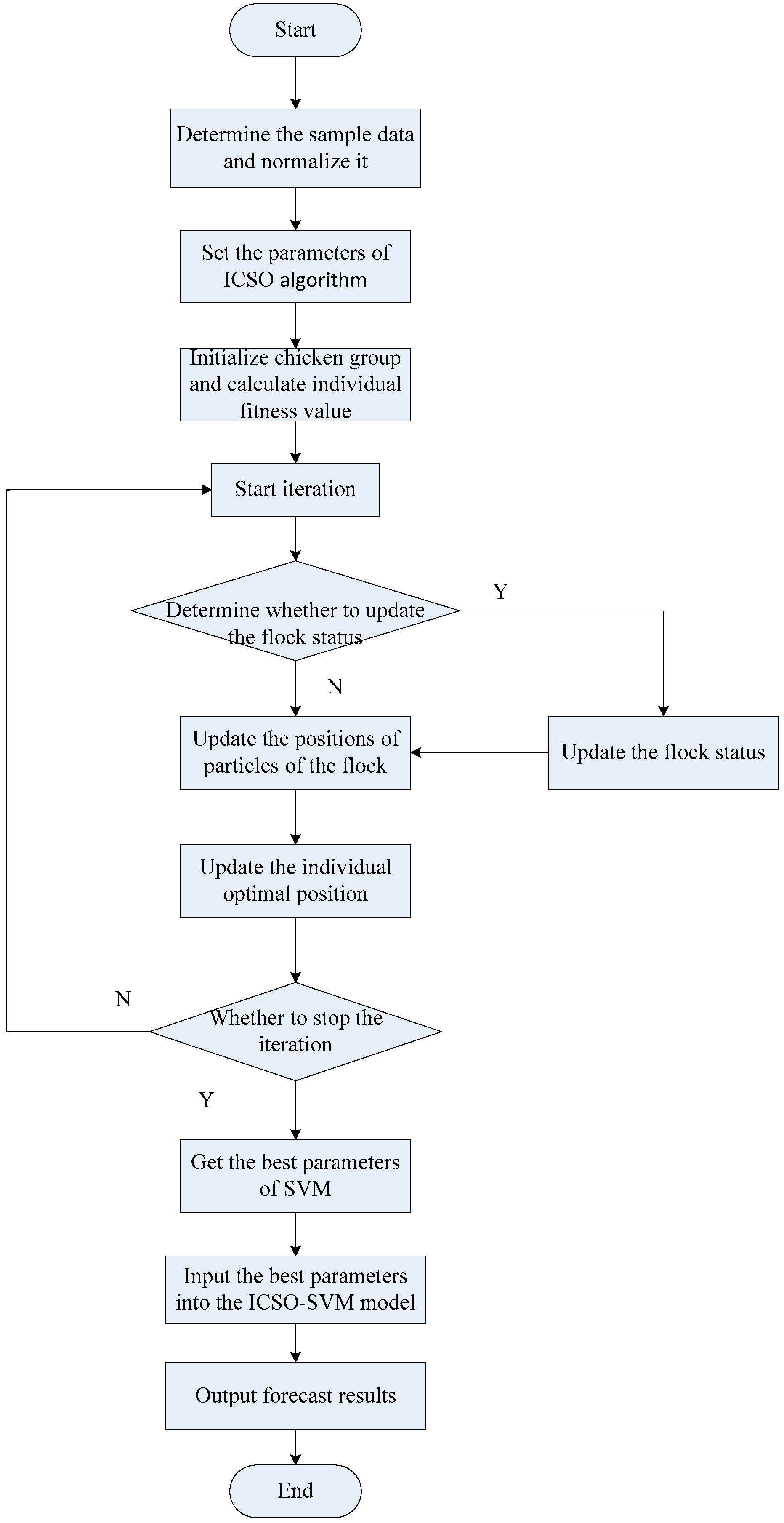
3. Simulation Experiment and Data Analysis

The basic idea of short-term wind power forecasting is as follows: firstly, the training samples and test samples are determined and normalized; secondly, the model is trained by using the training samples; finally, the test samples are predicted by the model and the evaluation indicators are used to evaluate the prediction effect of the model.

The la haute borne data provided by ENGIE Renewable Energy are used as experimental data in this study. The wind turbine name is R80711. The manufacturer of the wind turbine is the company SENVION, the rated power of the wind turbine is 2050 kw, the rotor diameter of the wind turbine is 82 m, and the hub height of the wind turbine is 80 m. A total of 540 sets of wind power data from 27 January to 30 January 2017 are selected as experimental data.

Table 4. The input and output of the prediction model.

Input	Output
Wind speed	Power
wind direction
Temperature

presents the input and output of the prediction model.

In Table 4, the wind speed, temperature and wind direction are selected as the input of the prediction model. The power is selected as output. The ICSO algorithm uses the mean square error of the training samples as the fitness function of. The calculation equation of fitness function is as follows:

$$Fit=\frac{1}{n}{{\displaystyle \sum _{i=1}^n(q_i-q_i^{*})}}^2$$

(14)

There are n training samples in total. q_i is the true value of training samples. $q_i^{*}$ is the prediction value of training samples.

In this study, the root mean square error (RMSE) and relative error (RE) are used to evaluate the prediction effect of the model:

$$RMSE=\sqrt{\frac{1}{N}{\displaystyle \sum _{i=1}^N{(o_i-o_i^{*})}^2}}$$

(15)

$$RE=\frac{o_i^{*}-o_i}{o_i}\times 100$$

(16)

where o_i is the true value of test samples, $o_i^{*}$ is the prediction value of test samples.

The specific steps to predict short-term power using the ICSO-SVM model are as follows:

(1)

Determine the input samples and test samples.

(2)

Normalize input and output samples.

(3)

Initialize chicken parameters and population, and calculate the fitness value of each particle.

(4)

Optimize SVM parameters with ICSO.

(5)

Input optimized parameters into the SVM model and predict the test samples.

(6)

Denormalize the predicted results and compare them with real values.

The prediction process of short-term power by the ICSO-SVM model is shown in Figure 3.

In order to compare the effects of the number of training samples on the prediction accuracy, two sets of wind power data are selected to test the model. The first set of wind power data consists of 540 samples, 500 samples are used to train the model, and 40 samples are used to test the model. The second set of wind power data consists of 440 samples, 400 samples are used to train the model, and 40 samples are used to test the model.

Firstly, the ICSO-SVM model and CSO-SVM model are tested with the first set of wind power data. The predicted results of the two models are shown in Figure 4.

As shown in Figure 4, the black line indicates the true value curve, the green line indicates the predicted curve of the CSO-SVM model, and the blue line indicates the predicted curve of the ICSO-SVM model. On the whole, the fluctuation trend of the blue line is closer to the fluctuation trend of the black line, especially between the 30th sample and the 40th sample. In particular in the later stage of prediction, the trend of blue line is more in line with the trend of black line than that of green line. The relative error percentage curves of the two models are shown in Figure 5.

As shown in Figure 5, the fluctuation of the blue line is stable, while the green line is more volatile. The maximum relative error percentage of CSO-SVM model is nearly 30%, which is obviously higher than that of ICSO-SVM model.

Secondly, ICSO-SVM model and CSO-SVM model are tested with the second set of wind power data. The predicted results of the two models are shown in Figure 6.

As shown in Figure 6, as the number of training samples decreases and the number of test samples increases. Compared with Figure 4, it can be found that the prediction errors of the two models are obviously increased. The predictive effect of ICSO model for the second set of wind power data is better than CSO-SVM model. The relative error percentage curves of the two models are shown in Figure 7.

Compared with Figure 5, it can be seen from Figure 7 that the maximum predicted relative error percentage of CSO-SVM exceeds 60%, and the maximum predicted relative error percentage of ICSO-SVM is close to 50%, indicating that the training sample has a greater impact on the prediction results.

For 500 training samples and 400 training samples, the maximum relative error percentages, minimum relative error percentages, average relative error percentages and root mean square errors of ICSO-SVM and CSO-SVM models are shown in

Table 5. Analysis of test results.

Number of Training Samples	Model	Maximum Relative Error Percentage %	Minimum Relative Error Percentage %	Average Relative Error Percentage %	RMSE
500	CSO-SVM	28.97	−13.65	9.30	40.53
	ICSO-SVM	15.75	−21.14	6.96	30.89
400	CSO-SVM	69.67	−9.63	18.29	51.52
	ICSO-SVM	57.71	−21.61	16.14	46.91

.

It can be seen from Table 5 that as the training samples decrease, the average relative error and the RMSE value increase significantly. For the first set of wind power data, the average relative error percentage of the CSO-SVM model is 9.30%. For the second set of wind power data, the average relative error percentage is 18.29%, which is nearly 2 times larger. The RMSE value of the CSO-SVM model increases from 40.53 to 51.52. The RMSE value of the ICSO-SVM model increases from 30.89 to 46.91. Through data analysis, it is found that the number of training samples has an obvious impact on the prediction effect of the model.

The test results show that the prediction errors of CSO-LSSVM and ICSO-SVM models increase relatively with the decrease of training samples. Whether the training samples are 500 or 400, the average relative error and RMSE value of the ICSO-SVM model are smaller than the CSO-SVM model.

4. Conclusions

The problems of air pollution and excessive exploitation of traditional fossil energy are becoming increasingly serious. It is imperative to develop clean energy. Because of its renewable, clean and environmental advantages, wind power generation receives attention from all over the world, especially in countries with energy shortages. The installed capacity of wind turbines has increased year by year. However, wind power has its own limitations and is greatly affected by the weather. If the electricity generated by the wind is directly integrated into the power grid, it will impact the quality of voltage and frequency of the power grid. The stable operation of the power grid is destroyed. Therefore, it is of practical significance to make predictions on short-term wind power and improve the stability of power system operation. The SVM has better robustness, can avoid dimension disaster and has strong non-linear mapping ability. So short-term wind power is predicted by SVM in this study.

In this study, the traditional CSO algorithm is improved. Wind power is predicted by the ICSO-SVM model. This study draws the following conclusions:

(1)

Because of the limitations of traditional CSO algorithm, both local search ability and global search ability need to be improved. So the ICSO algorithm is introduced in this study. In the ICSO algorithm, the position update equation of hens and chicks is improved. The self-learning factor is introduced into the hen position updating equation to improve search ability. The role of learning from the optimum particle is introduced into the chick position updating equation. So the local search ability and global search ability of the algorithm are improved.

(2)

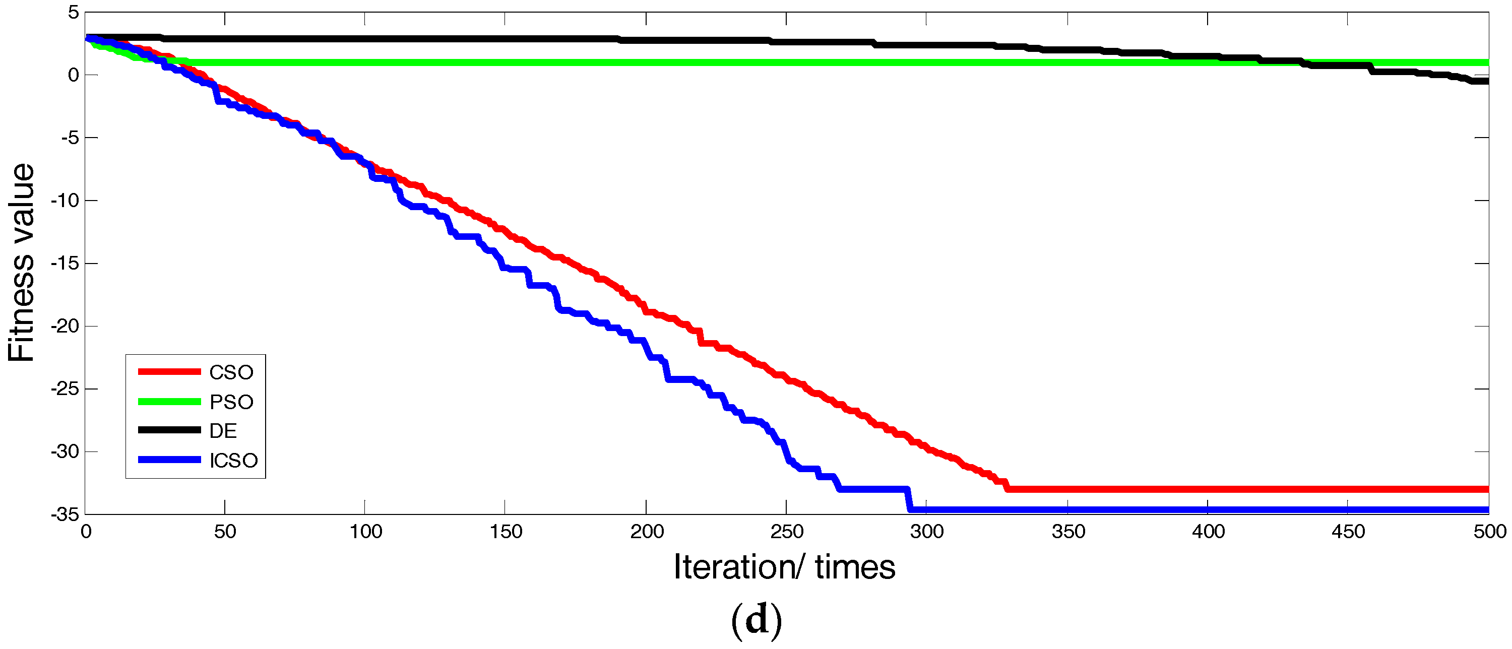
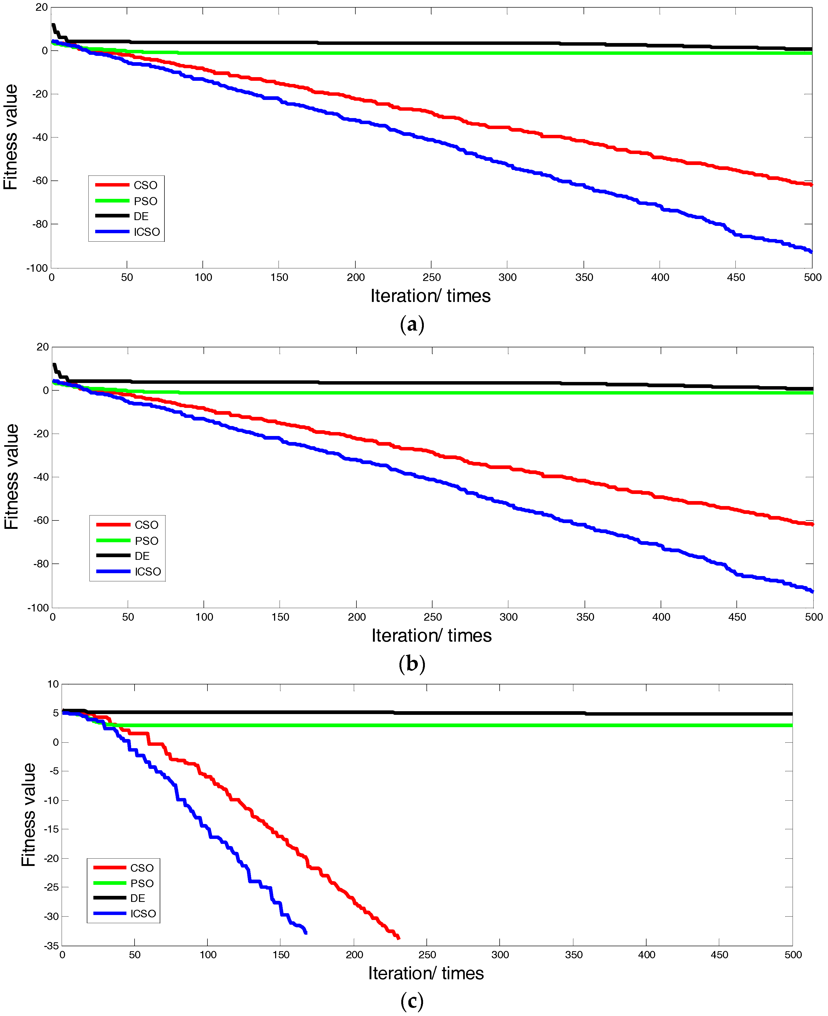
The PSO, CSO, DE and ICSO algorithms are tested by the four standard test functions and the test data are analysed. By comparing with the other three optimization algorithms, the ICSO algorithm has the best convergence accuracy, whether in the 20th or 80th dimension of the standard test functions.

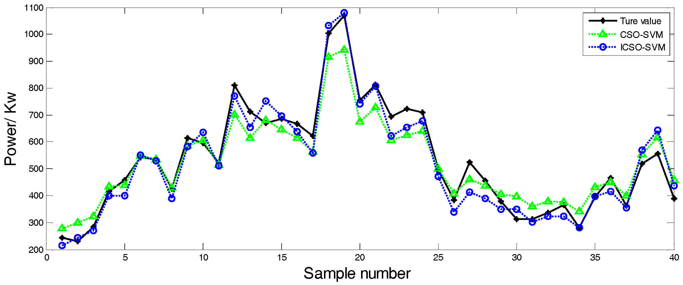
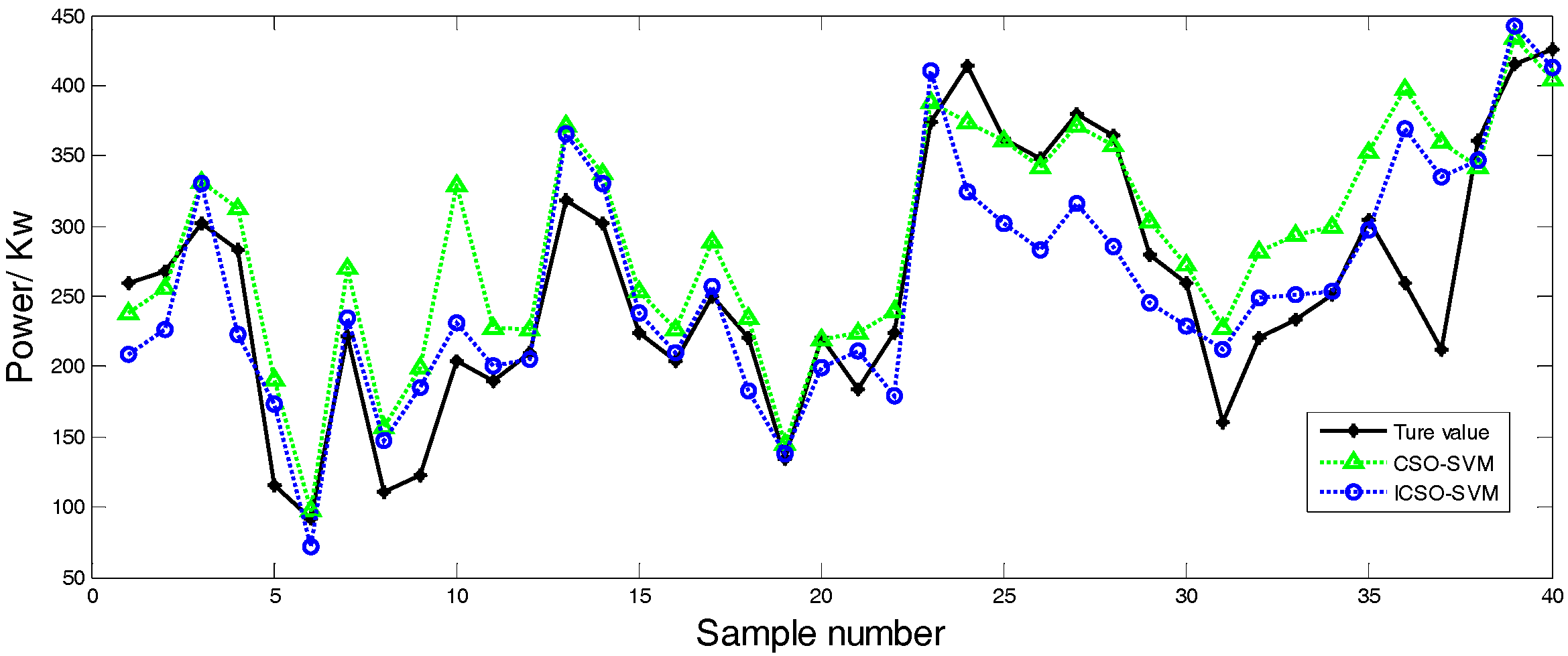
(3)

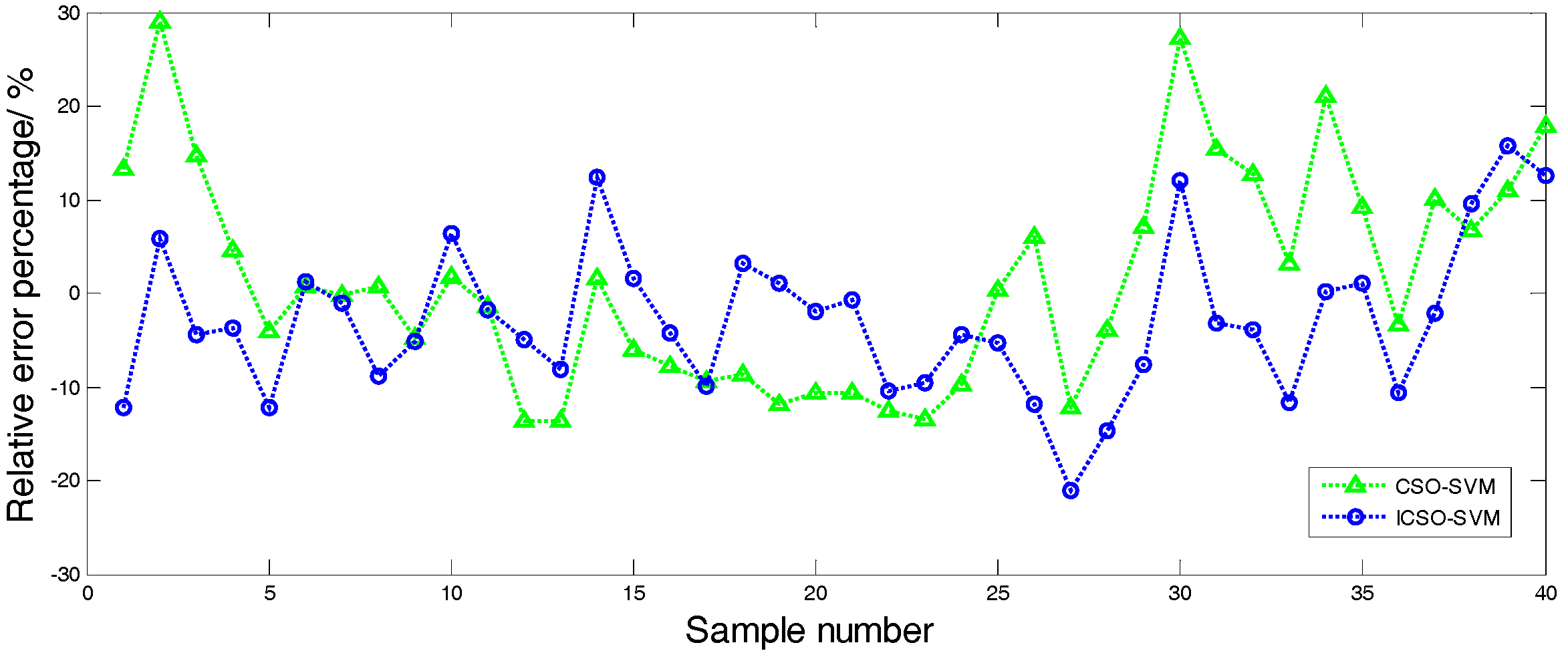
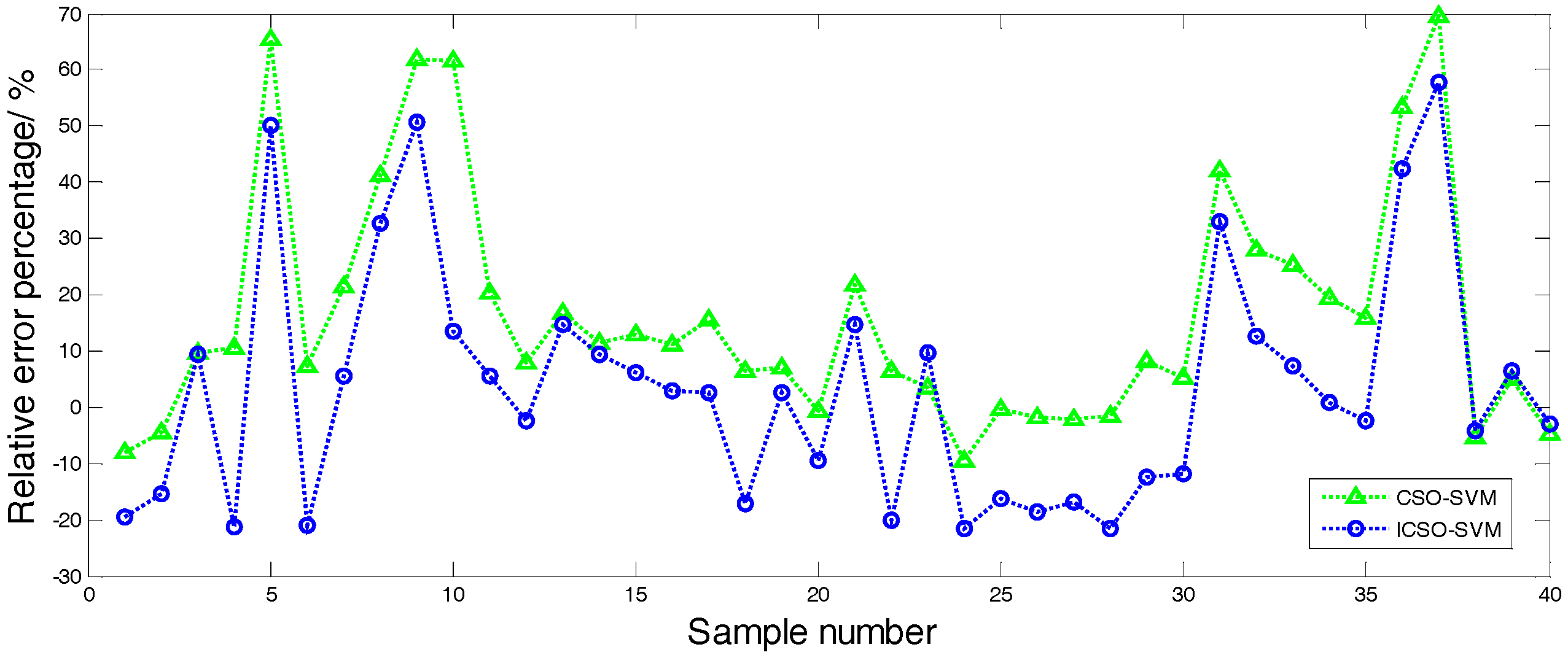
When the number of training samples is reduced from 500 to 400, the predicted average relative error percentage and RMSE values of the CSO-SVM and ICSO-SVM models are obviously increased. The results indicate that the number of training samples has a significant impact on the prediction effect, and show that ICSO-SVM has better prediction accuracy than the CSO-SVM model.

References

1. Kaid, I.E.; Hafaifa, A.; Guemana, M.; Hadroug, N.; Kouzou, A.; Mazouz, L. Photovoltaic System Failure Diagnosis Based on Adaptive Neuro Fuzzy Inference Approach: South Algeria Solar Power Plant. J. Clean. Prod. 2018, 204, 169–182. [Google Scholar] [CrossRef]
2. Cao, R.W.; Yuan, X.Y.; Jin, Y.; Zhang, Z. Mw-Class Stator Wound Field Flux-Switching Motor for Semidirect Drive Wind Power Generation System. IEEE Trans. Ind. Electron. 2019, 66, 795–805. [Google Scholar] [CrossRef]
3. Li, L.L.; Lin, G.Q.; Tseng, M.L.; Tan, K.H.; Lim, M.K. A Maximum Power Point Tracking Method for Pv System with Improved Gravitational Search Algorithm. Appl. Soft Comput. 2018, 65, 333–348. [Google Scholar] [CrossRef]
4. Li, L.L.; Chen, X.D.; Tseng, M.L.; Wang, C.H.; Wu, K.J.; Lim, M.K. Effective power management modeling of aggregated heating, ventilation, and air conditioning loads with lazy state switching. J. Clean. Prod. 2017, 166, 844–850. [Google Scholar] [CrossRef]
5. Zhan, J.; Wang, R.L.; Yi, L.Z.; Wang, Y.G.; Xie, Z.J. Health Assessment Methods for Wind Turbines Based on Power Prediction and Mahalanobis Distance. Int. J. Pattern Recognit. Artif. Intell. 2019, 33, 1951001. [Google Scholar] [CrossRef]
6. Zhang, K.Q.; Qu, Z.X.; Dong, Y.X.; Lu, H.Y.; Leng, W.N.; Wang, J.Z.; Zhang, W.Y. Research on a Combined Model Based on Linear and Nonlinear Features—A Case Study of Wind Speed Forecasting. Renew. Energy 2019, 130, 814–830. [Google Scholar] [CrossRef]
7. Li, L.L.; Cheng, P.; Lin, H.C.; Dong, H. Short-term output power forecasting of photovoltaic systems based on the deep belief net. Adv. Mech. Eng. 2017, 9, 1–13. [Google Scholar] [CrossRef]
8. Yang, M.; Chen, X.X.; Huang, B.Y. Ultra-Short-Term Multi-Step Wind Power Prediction Based on Fractal Scaling Factor Transformation. J. Renew. Sustain. Energy 2018, 10, 053310. [Google Scholar] [CrossRef]
9. Liu, Z.L.; Hajiali, M.; Torabi, A.; Ahmadi, B.; Simoes, R. Novel Forecasting Model Based on Improved Wavelet Transform, Informative Feature Selection, and Hybrid Support Vector Machine on Wind Power Forecasting. J. Ambient Intell. Hum. Comput. 2018, 9, 1919–1931. [Google Scholar] [CrossRef]
10. Naik, J.; Bisoi, R.; Dash, P.K. Prediction Interval Forecasting of Wind Speed and Wind Power Using Modes Decomposition Based Low Rank Multi-Kernel Ridge Regression. Renew. Energy 2018, 129, 357–383. [Google Scholar] [CrossRef]
11. Hong, D.Y.; Ji, T.Y.; Li, M.S.; Wu, Q.H. Ultra-Short-Term Forecast of Wind Speed and Wind Power Based on Morphological High Frequency Filter and Double Similarity Search Algorithm. Int. J. Electr. Power Energy Syst. 2019, 104, 868–879. [Google Scholar] [CrossRef]
12. Bhaskar, K.; Singh, S.N. AWNN-Assisted Wind Power Forecasting Using Feed-Forward Neural Network. IEEE Trans. Sustain. Energy 2012, 3, 306–315. [Google Scholar] [CrossRef]
13. Wang, Y.; Wang, H.B.; Srinivasan, D.; Hu, Q.H. Robust functional regression for wind speed forecasting based on Sparse Bayesian learning. Renew. Energy 2019, 132, 43–60. [Google Scholar] [CrossRef]
14. Wang, K.J.; Qi, X.X.; Liu, H.D.; Song, J.K. Deep belief network based k-means cluster approach for short-term wind power forecasting. Energy 2018, 165, 840–852. [Google Scholar] [CrossRef]
15. Li, C.B.; Lin, S.S.; Xu, F.Q.; Liu, D.; Liu, J.C. Short-Term Wind Power Prediction Based on Data Mining Technology and Improved Support Vector Machine Method: A Case Study in Northwest China. J. Clean. Prod. 2018, 205, 909–922. [Google Scholar] [CrossRef]
16. Shi, K.P.; Qiao, Y.; Zhao, W.; Wang, Q.; Liu, M.H.; Lu, Z.X. An Improved Random Forest Model of Short-Term Wind-Power Forecasting to Enhance Accuracy, Efficiency, and Robustness. Wind Energy 2018, 21, 1383–1394. [Google Scholar] [CrossRef]
17. Khorramdel, B.; Chung, C.Y.; Safari, N.; Price, G.C.D. A Fuzzy Adaptive Probabilistic Wind Power Prediction Framework Using Diffusion Kernel Density Estimators. IEEE Trans. Power Syst. 2018, 33, 7109–7121. [Google Scholar] [CrossRef]
18. Zheng, D.H.; Semero, Y.K.; Zhang, J.H.; Wei, D. Short-Term Wind Power Prediction in Microgrids Using a Hybrid Approach Integrating Genetic Algorithm, Particle Swarm Optimization, and Adaptive Neuro-Fuzzy Inference Systems. IEEJ Trans. Electr. Electron. Eng. 2018, 13, 1561–1567. [Google Scholar] [CrossRef]
19. Shi, W.G.; Guo, Y.; Yan, S.X.; Yu, Y.; Luo, P.; Li, J.X. Optimizing Directional Reader Antennas Deployment in Uhf Rfid Localization System by Using a Mpcso Algorithm. IEEE Sens. J. 2018, 18, 5035–5048. [Google Scholar] [CrossRef]
20. Wu, Z.Q.; Yu, D.Q.; Kang, X.H. Application of Improved Chicken Swarm Optimization for Mppt in Photovoltaic System. Optim. Control Appl. Methods 2018, 39, 1029–1042. [Google Scholar] [CrossRef]
21. Wu, Y.; Yan, B.; Qu, X.J. Improved Chicken Swarm Optimization Method for Reentry Trajectory Optimization. Math. Probl. Eng. 2018, 13, 8135274. [Google Scholar] [CrossRef]
22. Mygdalis, V.; Tefas, A.; Pitas, I. Exploiting Multiplex Data Relationships in Support Vector Machines. Pattern Recognit. 2019, 85, 70–77. [Google Scholar] [CrossRef]
23. Dong, C.Y.; Chen, J. Optimization of Process Parameters for Anaerobic Fermentation of Corn Stalk Based on Least Squares Support Vector Machine. Bioresour. Technol. 2019, 271, 174–181. [Google Scholar] [CrossRef] [PubMed]
24. Shang, C.F.; Wei, P.C. Enhanced Support Vector Regression Based Forecast Engine to Predict Solar Power Output. Renew. Energy 2018, 127, 269–283. [Google Scholar] [CrossRef]
25. Wei, J.W.; Dong, G.Z.; Chen, Z.H. Remaining Useful Life Prediction and State of Health Diagnosis for Lithium-Ion Batteries Using Particle Filter and Support Vector Regression. IEEE Trans. Ind. Electron. 2018, 65, 5634–5643. [Google Scholar] [CrossRef]
26. Singh, M.; Shaik, A.G. Faulty Bearing Detection, Classification and Location in a Three-Phase Induction Motor Based on Stockwell Transform and Support Vector Machine. Measurement 2019, 131, 524–533. [Google Scholar] [CrossRef]
27. Wang, X.K.; Guan, S.Y.; Hua, L.; Wang, B.; He, X.M. Classification of Spot-Welded Joint Strength Using Ultrasonic Signal Time-Frequency Features and PSO-SVM Method. Ultrasonics 2019, 91, 161–169. [Google Scholar] [CrossRef]
28. Meng, X.; Liu, Y.; Gao, X.; Zhang, H. A new bio-inspired algorithm: Chicken swarm optimization. Adv. Swarm Intell. 2014, 5, 86–94. [Google Scholar]
29. Hu, H.; Li, J.; Huang, J. Economic operation optimization of micro-grid based on chicken swarm optimization algorithm. High Volt. Appar. 2017, 53, 119–125. [Google Scholar]
30. Hong, Y.; Yu, F. Improved chicken swarm optimization and its application in coefficients optimization of multi-classifier. Comput. Eng. Appl. 2017, 53, 158–161. [Google Scholar]
Figure 1. Flow chart of improved chicken swarm optimization algorithm (ICSO).
Sustainability 11 00512 g001
Figure 2. The convergence curves: (a) the convergence curves of f1; (b) the convergence curves of f2; (c) the convergence curves of f3; (d) the convergence curves of f4.
Sustainability 11 00512 g002aSustainability 11 00512 g002b
Figure 3. The flow chart of short-term prediction.
Sustainability 11 00512 g003
Figure 4. The predicted results of the two models for 500 training samples and 40 test samples.
Sustainability 11 00512 g004
Figure 5. The relative error percentage for 500 training samples and 40 test samples.
Sustainability 11 00512 g005
Figure 6. The predicted results of the two models for 400 training samples and 40 test samples.
Sustainability 11 00512 g006
Figure 7. The relative error percentage for 400 training samples and 40 test samples.
Sustainability 11 00512 g007