Determinants of the Price of Housing in the Province of Alicante (Spain): Analysis Using Quantile Regression

Abstract

After almost a decade of crisis, the housing market in Spain shows significant signs of recovery, with increases in both the average price and the number of sales transactions. Housing is the main asset for the majority of households, and it also has the most resources devoted to it, thus, when it comes to buying a residence, people do not only look at the asset’s intrinsic characteristics, but also consider other particularities such as the neighbourhood, accessibility to services, availability of public transport or adequate funding. The study aimed to analyse and quantify the relationship that exists between the asking price of second-hand housing on the market in Alicante and the attributes that characterise them. This was done using a multivariate analysis to estimate a hedonic pricing model by ordinary least squares and a quantile regression to analyse the impact of the characteristics in different price ranges. The results show the segmentation of the prices in the Alicante market, with higher prices in the northern coastal area over the southern and inland comarcas.

1. Introduction

Housing is a primary need asset. The Spanish Constitution sustains, within its fundamental rights and duties, the “right to decent and adequate housing”. The most common type of tenure in Spain is property ownership, which represents approximately 76.7%, whether with or without a mortgage, while only 16.9% of dwellings are utilised for rental, and 6.4% correspond to other types of tenure [1].

Consumer goods are products that are acquired on the market at a certain price, with the objective of satisfying a need. Dwellings have a twofold consideration: on the one hand, as durable consumer goods, and, on the other hand, as an investment asset [2] (p. 46). This concept is old and was initialled by Keynes [3] (p. 75).

This study analysed the behaviour of the real estate market in the province of Alicante (Spain). To demonstrate the importance of this market in the territory studied, in Figure 1a, you can see the number of real estate transactions in the province of Alicante compared to provinces such as Madrid or Barcelona that have triple the number of inhabitants. Analysing the type of transactions in detail, there is a strong relevance of second-hand housing compared to new construction, which represents approximately 88% of the transactions in the 2014–2017 period. New construction was of great importance in years prior to the financial crisis of 2007, however, in recent years, it only represents 12% the transactions in the real estate market in the province of Alicante.

In a national context, during the last four years (2014–2017), the average prices of housing have been stable, a trend that is also extended to the province of Alicante (Figure 1b). However, this is not the case in Barcelona and Madrid, where prices show an upward trend. The data shown try to summarise the price of housing in a single mean value for an entire province. This simplification of reality provides a synthetic value that allows the study of its evolution but implies not considering the existing diversity in local markets or consumer preferences regarding the characteristics of housing.

In this study, we used a methodology based on the hedonic price model, which is a substantial body of historical research used to try to explain the value of housing based on the valuation of its components [5] (p. 3). The hedonic pricing method (HPM) is a procedure that allows you to set the characteristics that are determinant in the value of a heterogeneous asset, as is the case of a dwelling, as well as quantify the contribution of each one of them. The HPM has been used in the automotive market, with several authors highlighting the work of Court [6], to incorporate improvements to the methodology of analysis. The theoretical basis was developed by different authors, highlighting among others Lancaster [7], Ridker and Henning [8] and Rosen [9]. It is one of the globally most-used methodologies in the analysis of the real estate market, as well as its application to other markets such as the automotive or food sectors, to cite two examples.

The research objectives proposed were: (1) to estimate the impact of the characteristics of housing in the asking price, in the province of Alicante; and (2) to identify, for the same housing characteristic, the differences in seller valuations based on the asking price.

The first hypothesis that arose in the investigation is that there are certain characteristics of housing that have a greater effect on determining sales prices than others. A multitude of characteristics can influence the determination of the sales price, such as the dwelling’s intrinsic characteristics, the characteristics of the environment, the geographic location, etc. The second hypothesis proposed is that the same characteristic can be valued differently within the different ranges of property prices. For example, in housing with low prices, the relevance of having elevator should be higher than in those with a higher price.

The first objective was intended to be addressed through an analysis of ordinary least squares (OLS) regression, allowing the variables that are more relevant to the determination of the sales prices of multifamily housing projects in the province of Alicante to be determined. Several regression models were made to evaluate the incidence of including new variables, quantifying the improvement of the explanatory variability of the different models. Afterwards, a method was used that allows for the breakdown of the explanatory variability of each variable, thereby estimating the relative importance of each variable in the regression model. Lastly, the signs and the effects obtained in the statistically significant characteristics were analysed. OLS models are based on the conditional mean of the dependent variable given certain values of the predictor variables, but do not provide information for other conditional quantiles of the dependent variable.

The second objective was addressed through a method of quantile regression, which enables modelling different conditional quantiles of the dependent variable, overcoming the limitations of the OLS models. This way, it is possible to estimate the effect of each independent variable on different segments of the conditional distribution of the price of housing.

This paper contributes to the literature in several ways. Firstly, it presents an exhaustive review of the literature of recent years to identify the most relevant characteristics in the determination of the price of housing. Secondly, it includes a database of prices, with a large sample that describes the housing market in Alicante. Thirdly, the relative importance of the characteristics of the dwelling in the determination of the price was estimated, and the behaviour of the regression coefficients in the different price ranges was evaluated.

The results obtained in this study show that housing characteristics and building characteristics are very relevant in the determination of the price, as well as the characteristics of the location. Other socio-demographic characteristics and housing tenure also moderately influence the determination of the asking price of a home. From the quantile regression, it is noted that the characteristics of housing have a different effect depending on the quantile the price is in, finding different effects depending on the variable analysed.

The document is organised as follows. Section 2 presents a review of the literature and shows an overview of the determinants of housing prices. Section 3 describes the materials and method, detailing the sources used and the generated database. Section 4 provides the results, comparing various models obtained using OLS and another model using quantile regression. Section 5 is the discussion of the results. Section 6 synthesises the conclusions obtained.

2. Review of the Literature

There are studies showing the many characteristics that can be used as determinants of the price of housing, and how these can be grouped into categories. Smith et al. [10] (pp. 34–41) assumed that housing is composed of a series of special characteristics such as: durability, heterogeneity, spatial fixation and government involvement. Sirmans et al. [5] analysed one hundred and twenty-five articles that used hedonic models, collecting the variables that are significant to determine the price and its sign, comparing the coefficients by geographic location and examining the relationship between the price of housing and amount of time on the market. The study concludes in the grouping of variables in the following categories: (1) structural characteristics; (2) internal; (3) external; (4) environmental; (5) public services; (6) market, occupation and sales factors; and (7) funding.

Based on the classification suggested by Sirmans et al. [5], a classification for the variables adapted to this research was created (

Table 1. Variables used by other authors for the determination of the price of housing.

Category	Characteristics	References
Dwelling characteristics (A)	Dwelling typology	[11,12,13,14,15,16,17,18,19,20,21,22,23,24]
	Age of the dwelling	[12,16,18,19,20,21,22,23,24,25,26,27,28,29,30,31,32,33,34,35,36,37,38,39,40,41,42,43,44,45,46,47]
	Dwelling surface area	[11,13,15,16,18,20,21,22,23,24,26,27,28,29,30,31,33,34,35,36,37,38,39,41,42,43,44,45,46,48,49,50,51,52,53,54,55,56,57,58,59,60,61]
	Number of bedrooms	[11,13,14,17,19,20,21,23,24,28,31,34,41,50,56,61,62,63]
	Number of bathrooms	[14,20,23,24,31,38,49,55,57,61,64]
	Floor of the dwelling	[15,21,24,27,37,38,39,42,55,56,57,60,61]
	Terrace	[23,28,31,52,61]
	Wardrobe	[24,43,59]
	State of conservation	[11,16,22,23,24,28,30,34,59]
Features of the building (B)	Garage slot	[13,16,18,23,24,28,31,38,44,45,46,49,54,55,58,59,61,64]
	Elevator	[13,16,22,23,24,29,31,43,52,57,59]
	Swimming pool in the building	[13,18,22,31,54,57,58,59,60,61]
Characteristics of the location (C)	Location within the territory or the city	[13,16,24,31,35,36,38,39,41,44,45,46,48,54,56,58,61,62,64,65]
	Proximity to the coast	[24,25,48,66]
Characteristics of the neighbourhood (D)	Age of the population	[15,28]
	Number of Foreigners	[15,22,23,28,42,51,67]
	Level of studies	[15,21,25,50,57,67,68]
Market, occupation and sale characteristics (E)	Price	In all studies this is the dependent variable
	Use of the dwelling	[34,52,56]
	Housing tenure	[19]

, column Category). Five categories of variables were establish: (A) dwelling characteristics; (B) features of the building; (C) characteristics of the location; (D) characteristics of the neighbourhood; and (E) market, occupation, and sale characteristics. In these categories, the different characteristics that may have an impact on the sale price of a dwelling were organised.

Fifty-seven articles were selected, published between 2008 and 2018, which deal with identifying the characteristics of housing that can influence the determination of the price of a dwelling. These documents were analysed. Table 1 summarises the characteristics used that have proven to be statistically significant (at >95% level) in the corresponding models.

Sagner [26] analysed the characteristics that are determinant in the price of housing in the metropolitan area of Chile through the analysis of a sample of 419 observations for 17 years (1990–2007), concluding that 68–71% of the price was determined by the characteristics of the dwelling, with the most important variables being antiquity and the surface area.

Bohl et al. [27] analysed the real estate market of Munster during the period of 1999–2009, both for single family homes and housing projects. Their results show that the most important characteristics were surface area, the age of the property, quality of life and proximity to the centre. In single-family dwellings, typology and surface area of the plot were also significant.

Kaya and Atan [31] obtained 756,082 observations from the price database from the Central Bank of Turkey, for the period from December 2010 to June 2012. Although the document does not show the standardised betas as it uses only dichotomous variables, regression coefficients could be used to determine the relative importance of each variable. Noteworthy results are that the location component was an important factor: users were willing to pay a lot more for a dwelling in Istanbul as opposed to the rest of the locations. Of the remaining housing characteristics, the most important was the surface area, which increased the price of dwellings if it was greater than 250 m², penalising those with a lower surface area.

In another study conducted in Turkey, Yayar and Demir [18] collected data from the survey on household budgets for 2010 and used 3709 observations with 45 variables. It was clear that housing characteristics such as the typology, the availability of central heating, the type of flooring in the bathrooms and the floor the dwelling was located on were the most influential variables. For location variables, the most important ones were distance to banking services and educational centres. Alkan [33] analysed the housing market in Ankara with prices offered on webpages in 2011, had a sample of 149 observations and used different statistical techniques to conclude that location was the most relevant factor.

Quispe Villafuerte [55] obtained estimates of the value of the characteristics of a dwelling in Metropolitan Lima with a dataset of 188 single-family dwellings and 146 flats for January 2010. The results obtained show that the most important characteristics were the type of neighbourhood (socio-economic status) and dwelling characteristics (mainly surface area and bathrooms), with the surface area of the plot being of the utmost relevance in single family homes.

In Machala (Ecuador), Zambrano Monserrate [36] analysed the real estate market of apartments for rent in 2013, with a sample of 635 observations. The most important characteristics were those that refer to the utilities such as water supply and garbage disposal, while the most relevant location characteristic was distance to parks.

Nicodemo and Raya [29] studied how distribution of the attributes affects the price of housing over time through quantile estimates, between the years 2004 and 2007, for five major Spanish cities. It has a database with 21,517 observations, provided by a real estate agency. Two regression models were performed, the first with OLS estimates and the second with a quantile regression. They concluded that the variation in prices between 2004 and 2007 was mainly due to changes in regression coefficients (implicit value that individuals assign to each characteristic), rather than by differences in the characteristics of the homes sold during the same period. In addition, it was evident that the difference was greater in lower price percentiles than those in the higher percentiles.

McGreal and Taltavull de la Paz [52] analysed the attributes that were determinant in pricing using two statistical methodologies (spatio-temporal autoregressive STAR and general linear model GLM), trying to control the space and time random effects. They used a sample of 2,362,800 housing prices for 16 years (1995–2010), located in seven provinces in Spain. The results show that there are market characteristics that are particular to different regions. The value of the attributes changes over time, which is evidence of the economic cycle of the real estate market. In addition, it emphasises the importance of income, population, accessibility and structural characteristics, to explain the price of housing and spatial differences.

Keskin and Watkins [37] compared whether the experience of professionals from the real estate market was as effective as a statistical analysis, comparing the predictive analysis of real estate agents and other market analysts with an econometric analysis in Istanbul. To accomplish this goal, real estate agents and appraisers were consulted, in such a way that delimits the different sub-markets that make up the city. In addition, a hedonic regression with a linear model was performed, with prices and attributes of dwellings obtained from real estate portals on the Internet. The results did not reveal which method was more effective given that they both have a good capacity for prediction.

Zhang and Yi [60] studied the determinants in the price of residential housing in Beijing during the 2013–2015 period. To this end, they carried out an OLS and a quantile regression with a sample of 190,580 dwellings on a leading real estate portal in China. They concluded that the impact of the specific characteristics of a dwelling (surface area, number of rooms, sizes of the living room and green area of the complex) vary differently depending on the conditional distribution of housing prices.

Zahirovich-Herbert and Gibler [20] analysed how the construction of new real estate promotions affects the sales price of existing dwellings, using a hedonic regression model with OLS estimates. They concluded that, when a new home construction that is larger than the average is promoted, it has a positive effect on the existing real estate stock, especially on those with a low price.

Chasco Yrigoyen and Sanchez Reyes [15] analysed how air pollution and noise affects housing prices in the downtown area of Madrid through a quantile regression. As determinants, they used the structural attributes of housing, variables of accessibility, and characteristics of the social and environmental environment. There was a spatial quantile regression with nine deciles, where the autoregressive coefficients were very significant especially in the last two, corresponding to the dwellings with higher prices. On the other hand, more affordable housing (deciles 0.1 and 0.2), located in not-so-central areas, could have a spatial autocorrelation problem, which becomes evident in the lower explanatory power of the model. In all deciles, air pollution has a negative effect on price, but significantly in the more expensive properties. On the other hand, noise was not significant, except for luxury homes or the last decile located in the centre of Madrid, where the increase in noise carries an increase in the price. Fitch Osuna et al. [68] obtained similar results in Mexico; housing prices increase in more noisy areas, as location and demographic characteristics prevails over other factors.

From the studies analysed, it can be determined that most of them aimed to reveal what characteristics determine the price of housing, but there were also other documents whose purpose was to analyse how a particular characteristic affects the value of the property. A recent line of research in Europe focuses on analysing the influence of the energy rating of housing in the price [11,17,19,56,57,64]. Numerous other studies relate to the influence of location in the price of housing [22,25,38,39,50,51]. Xiao et al. [41] studied how prices of homes in Beijing change depending on atmospheric pollution. Stetler et al. [48] analysed the effect of the proximity of dwellings to forest fires in Montana. Other documents focus their attention on the ecological, scenic and entertainment value that housing in proximity to bodies of water has [32,35,47], or analyse how the price of housing is affected by proximity to landfill sites [42], train stops [28] or subway stations [49]. Wen et al. [40] analysed how school quality affects the price of housing. Agnew and Lyons [67] studied the variation in the price depending on proximity to locations that generate employment. Zahirovich-Herbert and Gibler [20] studied how newly constructed dwellings affect real estate stock. There is also research aimed at determining which statistical method was the best predictor of price [44,46]. Another purpose of the documents is to apply econometric models for the urban rating [16,34,54,59] or determine how much the price of land affects the price of housing [53].

3. Materials and Methods

3.1. Study Area

This study focused on the province of Alicante in the southeast of Spain. The province has an extension of 5817 km², distributed in nine comarcas (Comarcas are administrative units equivalent to the districts in England or the Kreise in Germany) and 141 municipalities (Figure 2a). It is the fifth Spanish province by number of inhabitants, with a total population of 1.8 million inhabitants, and the third in terms of number of real estate transactions, which shows a large housing market.

Figure 2b shows urban areas represented in red stains, where it is apparent that there are more built up areas on the Mediterranean coast, with greater dispersion in inland areas. There is a broad typological diversity in the various municipalities of the province, and even within each municipality. The predominant typology in the province is of compact and monocentric cities, but most tourist areas are dominated by more extensive urban developments. For example, in the city of Alicante there are differences between the traditional town with a compact development, and the area of Playa de San Juan with scattered high-rise buildings (Figure 3a,b). Regarding differences between municipalities, for example, urban development includes high-rise buildings in the city of Benidorm (Figure 3c), or scattered, low-rise developments of single-family and multifamily dwellings on the Orihuela Costa (Figure 3d).

3.2. Methodology

This study used two methods of regression, OLS and quantile regression. In this way, it was possible to compare the results obtained with both methods, and to identify the percentage of change in the price, against a unitary change in the variable that defines each characteristic (OLS), and the incidence of unitary changes of the characteristics in the different price ranges (quantile regression).

For both models, a semi-logarithmic functional form was chosen, as it lends certain advantages [69] (p. 80). The log transformation reduces problems of heteroscedasticity, improving the goodness of fit of the data; in addition, it facilitates the interpretation of the coefficients as they show the percentage variation in the dependent variable that would be obtained for each increase in a unit of the explanatory variable [5] (p. 4) [70] (pp. 193–194). Sirmans et al. [5] (p. 4) indicated that hedonic models are often estimated with semi-logarithmic forms, with the natural log of price used as the dependent variable.

The hedonic price method (HPM) is based on the existence of heterogeneous assets [7] (p. 134). This method aimed to determine which attributes or characteristics explain the price of second-hand housing on the Alicante market and the importance of each one of them [8]. To obtain the values for these attributes or parameters, the most used method is OLS. Freeman et al. [71] (pp. 327–331) indicated that this method presents the problem that it cannot estimate the marginal willingness to pay due to identification problems. However, this method is not always the most representative of the sample, if there are important extreme values or high variability [15] (p. 5). The advantage of quantile regression over the OLS method is that it can explain the importance of the determinants of the dependent variable at any point in the distribution [72] (p. 318), thus it looks less prejudiced as it does not require establishing hypotheses about the random disturbance [15] (p. 5). The OLS model is the following:

$$ln\left(P_i\right)={\alpha }_0+{\displaystyle \sum }_{j=1}^J{\beta }_j{X}_{ij}+{\displaystyle \sum }_{k=1}^K{\gamma }_k{D}_{ik}+{\displaystyle \sum }_{m=1}^M{\delta }_m{L}_{im}+{\epsilon }_i$$

(1)

where ln (P_i) is the Napierian logarithm of the advertised asking price for housing “i”; α is the fixed component, it does not depend on the market; β_j is the parameter to estimate related to the characteristic “j”; X_ij is the continuous variable that collects the characteristic “j” of the observation “i”; γ_k is the parameter to estimate related to the characteristic “k”; D_ik is the dummy variable that collects the characteristic “k” of the observation “i”; δ_m is the parameter to estimate related to the location “m”; L_im is the dummy variable that collects the location “m” of the observation “i”; and ε_i is the error term in the observation “i”.

In Equation (1), the term X_ij is a matrix of independent continuous variables that describe several characteristics of the dwelling, the building, the environment and the market (see

Table 2. Set of variables that make up the study, with their units and description.

Category	Characteristics	Unit	Description of the Variable	Used
Dwelling characteristics (A)	A_flat	dummy	Indicates whether the property has this typology: Flat or apartment, penthouse, duplex, studio flat	YES
	A_penthouse
	A_duplex
	A_studio_flat
	A_age	numerical	Age of the building (years) Number of years that have passed since it was built
	A_area_m2		Built dwelling surface (sqm) Gross square meters of the dwelling
	A_bedrooms		Number of bedrooms in the dwelling	NO
	A_bathrooms		Number of bathrooms	YES
	A_floor		Floor the dwelling was located on within the building
	A_terrace	dummy	Availability of terrace
	A_wardrobe		Availability of built-in wardrobes	NO
	A_good_condition		Classification that the seller assigns to the state of the dwelling, such as “good”	YES
	A_new_construction		Newly build housing that can be: a project, under construction, or less than 3 years old
	A_state_to_reform		Requires refurbishment
Features of the building (B)	B_parking	dummy	Availability of garage slot	YES
	B_elevator		Availability of elevator
	B_pool		Availability of swimming pool
Characteristics of the location (C)	C_Alicante	dummy	Identifier of the comarca: Alicante, Marina Alta, Marina Baja, Bajo Vinalopó, Bajo Segura, El Condado, Alcoy, Alto Vinalopó and Medio Vinalopó	YES
	C_Marina_Alta
	C_Marina_Baja
	C_Bajo_Vinalopo
	C_Bajo_Segura
	C_Condado
	C_Alcoy
	C_Alto_Vinalopo
	C_Medio_Vinalopo
	C_coastalregion		Identification of property location within a coastal region
	C_coastal_dist_km	numerical	Distance (km) from the property to the coast	NO
Characteristics of the neighbourhood (D)	D_elderly	numerical	Ratio of dependant elderly	YES
	D_foreigners		Ratio of foreign population
	D_no_studies		Ratio of population without education
	D_university		Ratio of the population with university studies
	D_students		Ratio of the population with primary and secondary studies	NO
Market, occupation and sale characteristics (E)	E_price	numerical	The property price offered by the seller (in Euro)	Dependent variable
	E_vacant_dwelling	numerical	Ratio of empty dwellings	NO
	E_main_dwelling		Ratio of main dwellings
	E_secondary_dwelling		Ratio of second dwellings	YES
	E_rented_dwelling		Ratio of housing for rent
	E_mortgaged_dwelling		Ratio of mortgaged housing	NO
	E_home_ownership		Home ownership ratio

); the term D_ik is a matrix of independent dummy variables that describe characteristics of the dwelling, the building and the location; and L_im is a matrix of independent dummy variables that describe localisation characteristics, whether they be comarcas or municipalities, that control the fixed effects due to the spatial location of the data.

The steps followed to estimate the OLS model are described below. A first step examined the bivariate correlations matrix and scatter charts, to identify the existence of linearity between variables. An analysis of ordinary least square regressions was subsequently performed using a stepwise method for the selection of variables. Since the database has observations with missing or incomplete data, it was decided to use the selection of cases according to listwise deletion. The possible presence of multicollinearity was studied from the correlation coefficients, the variance inflation factor (VIF) and condition indices. The Breusch–Pagan test and a scatter chart of residuals were used to assess the presence of heteroscedasticity, and the Kolmogorov–Smirnov test and a frequency diagram were used to study the normality of the residuals.

The quantile model has certain advantages over the OLS model, as it allows control over non-linearity, non-normality due to skewness, outliers and heteroscedasticity [15] (p. 1). In addition, it allows the implied value of each of the characteristics for different price ranges to be identified, as they can vary [5] (p. 4). In this way, it is possible to identify the different impacts that characteristics have on the ranges of sales prices.

To explain the quantile regression model [73,74], a multiple linear regression model was used as a basis, as follows (Equation (2)):

$$Y_i=X_i{\beta }_{\theta }+u_{\theta i}$$

(2)

where Y_i is the dependent variable; X_i is the matrix of independent variables; β_θ the vector of parameters to be estimated for the quantile θ; and u_θi is the random disturbance corresponding to the quantile θ.

According to Koenker and Bassett [73] (p. 38), let {X_i: i = 1,…, N} denote a sequence of (row) K vectors of a known design matrix, and suppose {Y_i: i = 1,…, N} is a random sample on the regression process u_i = Y_i − X_iβ having distribution function F. In this regression model, θ quantiles for the dependent variable were defined, given a series of X_i: Quant(Y_i|X_i) = X_iβ_θ, being Quant_θ(u_θi|X_i) = 0 the only imposed condition. The θth regression quantile, 0 < θ < 1, was defined as any solution to the minimisation problem of Equation (3):

$$\underset{\beta \in R^k}{\min }\left\{{\displaystyle \sum }_{i\in \left\{i:Y_i\ge X_i\beta \right\}}\theta \left|Y_i-X_i{\beta }_{\theta }\right|+{\displaystyle \sum }_{i\in \left\{i:Y_i<X_i\beta \right\}}\left(1-\theta \right)\left|Y_i-X_i{\beta }_{\theta }\right|\right\}$$

(3)

This non-linear equation was solved through a simplex linear programming model. The estimation of the parameters in the case of the quantile regression is carried out through the minimisation of weighted absolute deviations with asymmetric weights [75], whereas OLS minimises the sum of the squared residuals. The median regression is a particular case of the quantile regression in which θ = 0.5, and it is the only case in which the weights are symmetric.

To perform the quantile regressions the R package “quantreg” (version 5.36) [76] was used. The algorithmic method used to compute the fit is the modified version of Barrodale and Roberts’ method [77], and is described in detail in [78,79]. The goodness of fit of the quantile models was calculated based on absolute deviations by pseudo-R1 [80]. It is useful for comparing quantile models, but they are not comparable to the coefficient of determination R² obtained by OLS (which is based on the variance of the squared deviations). Pseudo-R1 is obtained as 1 minus the ratio between the sum of absolute deviations in the fully parameterised models and the sum of absolute deviations in the null (non-conditional) quantile model.

3.3. The Sources of Information

Three main sources of data were used: a real estate portal, the Real Estate Cadastre (Catastro Inmobiliario) and the National Institute of Statistics (Instituto Nacional de Estadística). From the real estate portal, information was collected about the offer prices and characteristics of the dwellings. The electronic headquarters of the Real Estate Cadastre [81] was used to calculate the age of the buildings, since these data are not available on the real estate portal. Finally, data from the 2011 Population and Housing Census [82], published by the National Institute of Statistics every ten years, were used to gather the socio-demographic characteristics of the population.

The first set of data was obtained from one of the most important real-estate portals in Spain (idealista.com). This portal has a long history and implementation throughout Spain, as it has advertised real estate since 2000 and has nearly 1.5 million ads for sale, rental and sharing. Other studies also use real estate portals to collect sales prices and characteristics of dwelling [15,28,30,67,83], due to the lack of information from other official sources. It is rare to have data of actual transactions, the most common dataset being obtained from the offer, with several authors suggesting the possibility of extrapolating the data obtained to the demand side [69,84]. Data were collected on the asking price offered within the market, the characteristics of the dwelling (construction typology, constructed surface area, number of bedrooms, bathrooms, etc.), characteristics of the building (garage slot, elevator and swimming pool), and characteristics of the location (geographical coordinates, municipality and comarca where the property was located).

An important characteristic in the literature that affects the price of a property is its age. This characteristic was not advertised on the real estate portal, thus it was necessary to obtain it by other means. The electronic headquarters of the Spanish Real Estate Cadastre was used, extracting the information for 412,900 plots throughout the province of Alicante, following the methodology developed by Mora García [85] (pp. 85–111). The data used were geographical coordinates, the constructed surface area and the age of each cadastral plot. From this information, a raster map was compiled, which served to obtain an approximate age of the construction in relation to the surrounding buildings. Since the coordinates provided by the real estate portal may have slight discrepancies with actual location (around 100 m), this option allowed the most realistic estimate of the antiquity of the property.

The last source of information used was the 2011 population and housing census, where socio-demographic data were obtained in terms of census tract. Data regarding the age of the population, level of education, foreign population, use and tenure of housing were used. Based on the geographical coordinates of each property, it was possible to assign a census tract and associate the data relating to it.

3.4. Data

A total of 64,039 multifamily dwelling offers were taken from the real estate portal during June and August 2017, though the data presented inconsistencies since the information published was provided by the advertising party. Ads were identified for whole buildings that were offered as a single dwelling, or 200 m² constructed surface area dwellings with no bedrooms. For this reason, a previous screening was carried out to identify properties with unlikely data. Subsequently, the sample was subjected to an analysis of univariate outliers, discarding properties that differ by more or less than three standard deviations in their respective classified variables (Z scores), the focus of which process was on the constructed surface area, price, number of bedrooms, bathrooms and building floor. After these processes, the initial sample was reduced to 56,307 buildings.

The data extracted from the Real Estate Cadastre and the data from the census of population and housing were added to the information about prices and characteristics of dwellings obtained from the real estate portal. Once the database was completed, those cases with missing data for some characteristics were excluded, resulting in a sample of 34,138 dwellings.

Table 2 lists the 40 variables collected for this research, arranged according to the five categories defined in Table 1. It also indicates the unit with which each variable was measured, a brief description of each and if it has been used in the final regression model.

Category A was made up of 14 variables that were used to define the characteristics of the dwelling. The first four were dummy variables, which were used to identify the typology of multifamily dwellings (flat or apartment, penthouse, duplex and studio flat), encoded with a value of 1 when they have that characteristic and 0 when they do not. The following five variables were quantitative and were used to define the age of the construction (in years), the constructed surface area (m²), the number of bedrooms, the number of bathrooms and the floor that the dwelling was located on within the building. The two following variables were dummy and refer to if the home has a terrace and fitted wardrobes. The last three in the category were also dummy and define the state of conservation, differentiating between new construction, second-hand in good condition, and second-hand needing refurbishing.

Category B was made up of three variables that were used to define the characteristics of the building. Differentiation was made if the house has a garage slot in the building, and if the building has an elevator and a swimming pool. The three have been defined as dummy variables, such that a value 0 indicates that they do not have that characteristic and 1 that they do.

Category C was composed of eleven variables, nine of which were used to quantify the differences throughout the territory. A variable was defined for each of the nine comarcas that make up the province of Alicante (Figure 2a). It was possible to estimate the price differences on a territorial scale (infra-provincial) by means of these nine variables that identify the comarcas. In total, 106 municipalities were used (35 of the 141 do not have data) to control the fixed effects due to the spatial location of the data. To assess the influence of proximity to the coast on prices, two variables were defined: the first indicates whether the property is located in a coastal municipality, and the second quantifies the shortest distance from the property to the coast, considering the journey by road (network distance).

Category D brings together five variables that describe the characteristics of the neighbourhood. They were quantitative variables and were all expressed in ratios. They refer to characteristics of the census tract where the property was located. The dependant elderly ratio was calculated as the ratio of the sum of the population aged 65 or over for any given area, and the sum of the population aged between 16 and 64 in the same area. The ratio of foreign population was calculated as the ratio of the sum of the foreign population that resides in an area, and the sum of the total population in that area. To characterise the level of education, three variables were established: ratio of population without education or illiterate, population with primary and secondary education, and ratio of population with university education. Each ratio was calculated as the ratio of the sum of the population with that level of education that resides in an area, and the sum of the total population in that area.

Finally, Category E included six variables that describe the characteristics related to the market, occupation and sale. They were quantitative variables, all of which were expressed in ratios. Variables related to the use and tenure of housing were used. Three uses were established: vacant homes, main dwellings (used routinely by its owners) and second homes (vacation homes). In relation to land tenure, three types were established: rental housing (the owner was leasing the property), mortgaged housing (the user was the owner of the home but has outstanding mortgage payments), and home ownership (the user was the owner of the home that was fully paid for).

The descriptive statistics for all variables are shown in

Table 3. Descriptive statistics for the variables.

Cat.		Continuous Variables				Dummies Variables
	Characteristics	Mean	SD	Min.	Max.	Coding.	Freq.	Percent.
Dwelling (A)	A_flat						30,140	88.3
	A_penthouse						2328	6.8
	A_duplex						1179	3.5
	A_studio_flat						491	1.4
	A_age	31.2	11.3	1.0	93.1
	A_area_m2	95.3	31.8	20.0	249.0
	A_bedrooms	2.6	0.9	0.0	5.0
	A_bathrooms	1.6	0.6	0.0	4.0
	A_floor	2.9	2.5	0.0	20.0
	A_terrace					No Terrace With Terrace	14,932 19,206	43.7 56.3
	A_wardrobe					No wardrobe Wardrobe	12,743 21,395	37.3 62.7
	A_good_condition						32,069	93.9
	A_new_construction						255	0.8
	A_state_to_reform						1814	5.3
Building (B)	B_parking					No garage With garage	21,055 13,083	61.7 38.3
	B_elevator					No elevator With elevator	8715 25,423	25.5 74.5
	B_pool					No pool With pool	20,296 13,842	59.5 40.5
Location (C)	C_Alicante						12,674	37.1
	C_Marina_Alta						3833	11.2
	C_Marina_Baja						3938	11.5
	C_Bajo_Vinalopo						4276	12.5
	C_Bajo_Segura						7165	21.0
	C_Condado						137	0.4
	C_Alcoy						905	2.7
	C_Alto_Vinalopo						327	1.0
	C_Medio_Vinalopo						883	2.6
	C_coastalregion					Non-coastal Coastal	8636 25,502	25.3 74.7
	C_coastal_dist_km	5.78	10.37	0.00	54.90
Neighbourhood (D)	D_elderly	0.30	0.19	0.00	1.05
	D_foreigners	0.24	0.21	0.00	0.93
	D_no_studies	0.07	0.05	0.00	0.37
	D_university	0.17	0.10	0.00	0.54
	D_students	0.61	0.10	0.00	0.86
Market, etc (E)	price	131,039	80,061	15,000	610,000
	price_ln	11.61	0.59	9.62	13.32
	E_vacant_dwelling	0.16	0.13	0.00	0.68
	E_main_dwelling	0.57	0.27	0.10	1.00
	E_secondary_dwelling	0.27	0.25	0.00	0.84
	E_rented_dwelling	0.13	0.11	0.00	0.53
	E_mortgaged_dwelling	0.39	0.17	0.04	0.96
	E_home_ownership	0.42	0.16	0.00	0.83

.

Regarding the distribution of prices (Figure 4a), it can be observed that the littoral strip concentrated unit prices (€/m²) higher than the rest of the province of Alicante. This map shows the distribution of the average unit price by municipalities, using a minimum of 10 real estate prices to determine an average value. The municipalities in white have fewer than 10 dwellings, whereby they were omitted. The largest number of properties were concentrated in the municipality of Alicante (provincial capital), followed by other coastal municipalities (Figure 4b), showing the areas where there was greater activity in the real estate market.

Table 4. Average (€) and unit (€/m²) prices, by province and comarca.

	Zone	N (%)	Average Price € (SD)	Unit Price €/m2 (SD)
	Province of Alicante	34,138 (100%)	131,039 (80,060)	1390 (687)
Coastal area	Marina Alta	3833 (11.2%)	162,816 (88,418)	1754 (741)
	Marina Baja	3938 (11.5%)	155,244 (83,295)	1829 (692)
	Alicante	12,674 (37.1%)	149,077 (85,498)	1427 (667)
	Bajo Vinalopó	4276 (12.5%)	111,428 (63,235)	1157 (575)
	Bajo Segura	7165 (21.0%)	98,323 (54,090)	1239 (544)
Inland area	Condado	137 (0.4%)	86,903 (49,904)	807 (334)
	Alcoy	905 (2.7%)	75,502 (44,883)	734 (337)
	Alto Vinalopó	327 (1.0%)	75,402 (42,474)	711 (341)
	Medio Vinalopó	883 (2.6%)	71,042 (37,342)	695 (323)

Notes: N, sample size; SD, Standard Deviation.

shows that only three of the nine comarcas in Alicante (the three coastal areas) have a price higher than the provincial average. The average market price in the province of Alicante was 131,039 € (1390 €/m²), but there was evidence of significant differences between coastal (higher prices) and inland comarcas (lower prices).

The most represented typology in the sample were flats, with 30,140 units, of which 75% have an elevator and an average asking price of 142,257 € (1,505 €/m²).

Table 5. Average (€) and unit (€/m²) prices by typology of housing and availability of elevator.

	Total by Typology	Without /with Elevator	Average Price € (SD)		Unit Price €/m2 (SD)
Typology	N (%)	%/%	no elevator	with elevator	no elevator	with elevator
flat	30,140 (88.3%)	25.0/75.0	81,650 (54,609)	142,257 (77,293)	967 (596)	1505 (664)
penthouse	2328 (6.8%)	15.8/84.2	115,169 (76,454)	185,014 (98,239)	1270 (684)	1634 (674)
duplex	1179 (3.5%)	59.5/40.5	151,423 (69,715)	204,958 (90,011)	1360 (536)	1625 (634)
studio flat	491 (1.4%)	21.0/79.0	64,933 (39,548)	69,876 (50,707)	1347 (541)	1569 (650)
Total	34,138 (100%)	25.5/74.5	88,484 (60,265)	145,626 (80,798)	1016 (608)	1518 (665)

Notes: N, sample size; SD, Standard Deviation.

shows differences in the sales prices according to typology and availability of an elevator.

4. Results

4.1. OLS Hedonic Price Models

Of the variables described in Table 2, those evidencing multicollinearity problems with other variables were discarded, as in the case of the number of bedrooms with the constructed surface area, or the ratio of main and vacant dwellings to secondary homes. For this reason, seven variables were discarded: number of bedrooms (A_bedrooms), ratio of the population with primary and secondary education (D_students), ratio of vacant and main homes (E_vacant_dwelling and E_main_dwelling), ratio of mortgaged and owned property (E_mortgaged_dwelling and E_home_ownership), and distance to coast (C_coastal_dist_km). The fitted wardrobes (A_wardrobe) variable, despite being statistically significant, had a low explanatory power in the model, whereby it was ruled out to simplify the model (principle of parsimony).

Following the line of other authors [35,40,42,47,57,86,87], six regression models were made to evaluate the incidence of including new variables (grouped by categories), quantifying the explanatory improvement of the different models. Afterwards, a method was used that allows for the breakdown of the explanatory variability of each variable, thereby estimating the relative importance of each of them in the regression model. Once the six models were evaluated, Model 5 was adopted as definitive, and was taken as reference for the quantile regression.

Table 6. OLS regression models, according to variables introduced.

	Characteristics	Model 1 OLS	Model 2 OLS	Model 3 OLS	Model 4 OLS	Model 5 OLS	Model 6 OLS
	(Intercept)	10.574 *** (0.011)	10.205 *** (0.011)	10.056 *** (0.013)	9.961 *** (0.013)	10.010 *** (0.012)	9.849 *** (0.154)
A	A_flat			Reference
	A_penthouse	0.021 * (0.010)	0.074 *** (0.009)	0.091 *** (0.008)	0.107 *** (0.007)	0.116 *** (0.007)	0.119 *** (0.007)
	A_duplex	−0.028 * (0.013)	0.076 *** (0.012)	0.073 *** (0.011)	0.050 *** (0.010)	0.040 *** (0.010)	0.036 *** (0.010)
	A_studio_flat	−0.187 *** (0.020)	−0.246 *** (0.018)	−0.259 *** (0.016)	−0.309 *** (0.015)	−0.309 *** (0.015)	−0.315 *** (0.014)
	A_age	−0.006 *** (0.0002)	0.001 *** (0.0002)	0.001 ** (0.0002)	−0.0002 (0.0002)	−0.001 *** (0.0002)	−0.0003 (0.0002)
	A_area_m2	0.005 *** (0.0001)	0.006 *** (0.0001)	0.006 *** (0.0001)	0.006 *** (0.0001)	0.006 *** (0.0001)	0.006 *** (0.0001)
	A_bathrooms	0.342 *** (0.006)	0.224 *** (0.005)	0.239 *** (0.005)	0.231 *** (0.004)	0.236 *** (0.004)	0.233 *** (0.004)
	A_floor	0.037 *** (0.001)	0.013 *** (0.001)	0.005 *** (0.001)	0.004 *** (0.001)	0.002 * (0.001)	0.002 ** (0.001)
	A_terrace	0.236 *** (0.005)	0.117 *** (0.005)	0.070 *** (0.004)	0.052 *** (0.004)	0.041 *** (0.004)	0.037 *** (0.004)
	A_good_condition			Reference
	A_new_construction	0.194 *** (0.028)	0.105 *** (0.025)	0.186 *** (0.022)	0.166 *** (0.020)	0.177 *** (0.020)	0.163 *** (0.020)
	A_state_to_reform	−0.379 *** (0.011)	−0.251 *** (0.010)	−0.229 *** (0.009)	−0.223 *** (0.008)	−0.218 *** (0.008)	−0.217 *** (0.008)
B	B_parking		0.168 *** (0.005)	0.156 *** (0.004)	0.149 *** (0.004)	0.142 *** (0.004)	0.133 *** (0.004)
	B_elevator		0.284 *** (0.005)	0.244 *** (0.005)	0.241 *** (0.005)	0.231 *** (0.005)	0.232 *** (0.004)
	B_pool		0.308 *** (0.005)	0.207 *** (0.005)	0.137 *** (0.004)	0.119 *** (0.005)	0.124 *** (0.004)
C	C_Alicante				Reference
	C_Marina_Alta			0.132 *** (0.007)	0.076 *** (0.007)	0.058 *** (0.007)
	C_Marina_Baja			0.146 *** (0.007)	0.197 *** (0.007)	0.143 *** (0.007)
	C_Bajo_Vinalopo			0.043 *** (0.007)	0.099 *** (0.006)	0.030 *** (0.007)
	C_Bajo_Segura			−0.108 *** (0.006)	−0.130 *** (0.007)	−0.186 *** (0.007)
	C_Condado			−0.098 ** (0.030)	−0.082 ** (0.028)	−0.146 *** (0.028)
	C_Alcoy			−0.182 *** (0.013)	−0.166 *** (0.012)	−0.221 *** (0.012)
	C_Alto_Vinalopo			−0.156 *** (0.020)	−0.078 *** (0.019)	−0.144 *** (0.018)
	C_Medio_Vinalopo			−0.213 *** (0.013)	−0.149 *** (0.012)	−0.202 *** (0.012)
	C_coastalregion			0.315 *** (0.006)	0.202 *** (0.005)	0.129 *** (0.006)	0.068 *** (0.010)
D	D_elderly				0.343 *** (0.011)	0.282 *** (0.012)	0.244 *** (0.012)
	D_foreigners				0.238 *** (0.013)	0.108 *** (0.014)	−0.038 * (0.016)
	D_no_studies				−0.910 *** (0.045)	−0.874 *** (0.045)	−0.722 *** (0.046)
	D_university				1.112 *** (0.024)	0.996 *** (0.024)	1.021 *** (0.024)
E	E_secondary_dwelling					0.321 *** (0.010)	0.335 *** (0.012)
	E_rented_dwelling					0.201 *** (0.021)	0.195 *** (0.023)
	Spatial fixed effects	No	No	Yes (by comarcas)	Yes (by comarcas)	Yes (by comarcas)	Yes (by municipality)

Notes: dependent variable price_ln; N = 34,138; *** p < 0.001, ** p < 0.01, * p < 0.05; standard errors in parentheses.

shows the regression models using OLS, generated according to the characteristics grouped by categories. Model 1 was built only with the characteristics of dwellings, allowing explanation of 44.0% of the variability of the price (

Table 7. Descriptive statistics for the OLS regression models.

	Statistics	Model 1 OLS	Model 2 OLS	Model 3 OLS	Model 4 OLS	Model 5 OLS	Model 6 OLS
	R2	0.440	0.568	0.654	0.706	0.715	0.731
	adj. R2	0.439	0.568	0.654	0.706	0.715	0.730
	Std. Error	0.441	0.387	0.347	0.320	0.315	0.306
	F (sig.)	2676.7 (p < 0.001)	3449.9 (p < 0.001)	2935.0 (p < 0.001)	3154.3 (p < 0.001)	3054.7 (p < 0.001)	732.5 (p < 0.001)

). Reviewing standardised beta coefficients (

Table A1. Standardised Beta coefficients of the OLS regression models.

		Model 1 OLS	Model 2 OLS	Model 3 OLS	Model 4 OLS	Model 5 OLS
A	A_flat			Reference
	A_penthouse	0.009	0.032	0.039	0.046	0.050
	A_duplex	−0.009	0.024	0.023	0.016	0.012
	A_studio_flat	−0.038	−0.050	−0.052	−0.062	−0.062
	A_age	−0.111	0.022	0.010	−0.004	−0.013
	A_area_m2	0.266	0.300	0.317	0.302	0.317
	A_bathrooms	0.319	0.209	0.224	0.216	0.221
	A_floor	0.155	0.054	0.020	0.016	0.007
	A_terrace	0.199	0.098	0.059	0.044	0.035
	A_good_condition			Reference
	A_new_construction	0.028	0.015	0.027	0.024	0.026
	A_state_to_reform	−0.144	−0.096	−0.087	−0.085	−0.083
B	B_parking		0.139	0.129	0.123	0.117
	B_elevator		0.210	0.181	0.178	0.171
	B_pool		0.257	0.172	0.114	0.099
C	C_Alicante				Reference
	C_Marina_Alta			0.071	0.041	0.031
	C_Marina_Baja			0.079	0.107	0.078
	C_Bajo_Vinalopo			0.024	0.056	0.017
	C_Bajo_Segura			−0.075	−0.090	−0.129
	C_Condado			−0.011	−0.009	−0.016
	C_Alcoy			−0.050	−0.045	−0.060
	C_Alto_Vinalopo			−0.026	−0.013	−0.024
	C_Medio_Vinalopo			−0.057	−0.040	−0.054
	C_coastalregion			0.232	0.149	0.095
D	D_elderly				0.111	0.091
	D_foreigners				0.085	0.039
	D_no_studies				−0.079	−0.076
	D_university				0.182	0.163
E	E_secondary_dwelling					0.136
	E_rented_dwelling					0.036

Notes: dependent variable price_ln.

), the three variables of greater explanatory power, listed in order of relevance, were: the number of bathrooms, the constructed surface area and the availability of a terrace. All of them were statistically significant and showed a positive sign, such that the greater the number of bathrooms, or the availability of a terrace, the higher the price of housing.

Model 2 was built with the characteristics of the dwelling and the building. The explanatory power of the model increased dramatically, from 44.0% to 56.8%. According to the standardised beta coefficients, the most important characteristics were the constructed surface area, and the availability of a pool and elevator (Table A1). All variables were statistically significant and had the expected sign, except for antiquity, which obtained a positive sign. In this model, the characteristics of the building exercised a great influence on explaining variability in price.

In Model 3, the location characteristics, as in the comarca where the property was located, were added, increasing the percentage of explained variance to 65.4%. The most influential variables in this model were constructed surface area, coastal municipality and number of bathrooms. Regarding the location variables, it was apparent that coastal comarcas located to the north of the province (Marina Alta and Marina Baja) had a higher price than in the case of the comarca of Alicante (reference), while, in the comarcas located in the south or in the inland areas of the province, prices were lower.

In Model 4, neighbourhood characteristics (socio-demographic characteristics) were added, obtaining a coefficient of determination of 70.6%. In this case, the three most important variables were constructed surface area, number of bathrooms and the ratio of people with a university education. It was evident that the socio-demographic characteristics of the neighbourhood had some relevance in determining the price.

Model 5 was made up of five categories, represents the final model object of study and showed a slight increase in the explanatory power compared to the previous one, peaking at 71.5% (Table 7). The regression model reached a high level of robustness and relevance in the estimated parameters, making it acceptable for making inferences. To assess the existence of heteroscedasticity, a Breusch–Pagan test was performed, leading to the rejection of the null hypothesis of homoscedasticity (BP = 1239.4, df = 28, p < 0.001), and the heteroscedasticity prevalence. Upon analysis of the residuals scatter plot, there was no evidence of serious problems of heteroscedasticity, showing a random distribution of residuals (Figure A1b). The normality of the residuals was contrasted with the Kolmogorov–Smirnov test, rejecting the null hypothesis of normality (D = 0.192, p < 0.001). Reviewing the diagram of frequencies, a certain normality of residuals was observed (Figure A1a). For the analysis of the collinearity of the variables, the variance inflation factor (VIF) statistic was used. Several authors have suggested that there are collinearity problems if the VIF is greater than 10 [88] (p. 363) [89] (pp. 28–29). Most values were close to 1 (

Table A2. Full details of the regression for the Model 5 OLS.

		Unstandardised Coefficients		Std Coef.			95.0% CI for B		Collinearity Statistics
		B	Std. Error	Beta	t	Sig.	Lower Bound	Upper Bound	Tolerance	VIF
	(Intercept)	10.010	0.012		802.6	0.000	9.986	10.035
A	A_flat	Reference
	A_penthouse	0.116	0.007	0.050	16.3	0.000	0.102	0.130	0.90	1.11
	A_duplex	0.040	0.010	0.012	4.0	0.000	0.020	0.059	0.88	1.13
	A_studio_flat	−0.309	0.015	−0.062	−21.1	0.000	−0.338	−0.280	0.96	1.04
	A_age	−0.001	0.0002	−0.013	−3.5	0.001	−0.001	0.000	0.63	1.59
	A_area_m2	0.006	0.0001	0.317	80.3	0.000	0.006	0.006	0.54	1.86
	A_bathrooms	0.236	0.004	0.221	56.4	0.000	0.228	0.244	0.55	1.83
	A_floor	0.002	0.001	0.007	2.0	0.041	0.000	0.003	0.81	1.24
	A_terrace	0.041	0.004	0.035	10.8	0.000	0.034	0.049	0.81	1.23
	A_good_condition	Reference
	A_new_construction	0.177	0.020	0.026	8.8	0.000	0.138	0.216	0.98	1.02
	A_state_to_reform	−0.218	0.008	−0.083	-28.0	0.000	−0.234	−0.203	0.95	1.05
B	B_parking	0.142	0.004	0.117	34.7	0.000	0.134	0.150	0.74	1.36
	B_elevator	0.231	0.005	0.171	51.2	0.000	0.222	0.240	0.75	1.33
	B_pool	0.119	0.005	0.099	26.5	0.000	0.110	0.128	0.59	1.68
C	C_Alicante	Reference
	C_Marina_Alta	0.058	0.007	0.031	8.4	0.000	0.045	0.072	0.61	1.64
	C_Marina_Baja	0.143	0.007	0.078	20.6	0.000	0.130	0.157	0.59	1.69
	C_Bajo_Vinalopo	0.030	0.007	0.017	4.5	0.000	0.017	0.044	0.59	1.71
	C_Bajo_Segura	−0.186	0.007	−0.129	−27.7	0.000	−0.199	−0.173	0.39	2.59
	C_Condado	−0.146	0.028	−0.016	−5.3	0.000	−0.200	−0.092	0.95	1.05
	C_Alcoy	−0.221	0.012	−0.060	−18.5	0.000	−0.245	−0.198	0.78	1.28
	C_Alto_Vinalopo	−0.144	0.018	−0.024	−7.8	0.000	−0.180	−0.108	0.90	1.11
	C_Medio_Vinalopo	−0.202	0.012	−0.054	−16.7	0.000	−0.226	−0.179	0.79	1.27
	C_coastalregion	0.129	0.006	0.095	22.0	0.000	0.118	0.141	0.45	2.23
D	D_elderly	0.282	0.012	0.091	23.6	0.000	0.259	0.306	0.56	1.80
	D_foreigners	0.108	0.014	0.039	7.6	0.000	0.080	0.136	0.32	3.09
	D_no_studies	−0.874	0.045	−0.076	−19.6	0.000	−0.962	−0.786	0.56	1.79
	D_university	0.996	0.024	0.163	42.2	0.000	0.950	1.043	0.56	1.79
E	E_secondary_dwelling	0.321	0.010	0.136	31.6	0.000	0.301	0.341	0.45	2.20
	E_rented_dwelling	0.201	0.021	0.036	9.4	0.000	0.159	0.244	0.57	1.76

Notes: dependent variable price_ln; N = 34,138; CI, Confidence Interval; VIF, Variance Inflation Factor.

), reaching a maximum value of 3.09, thus it was interpreted that there was no evidence of the existence of serious collinearity among the variables.

The variable that reached the highest VIF value was the ratio of foreign population, with correlations with other variables such as the elderly-dependency ratio (D_elderly) being observed, with a Pearson correlation coefficient r = 0.444; the ratio of second homes (E_secondary_dwelling) with r = 0.500; the ratio of rented housing (E_rented_dwelling) with r = 0.425; being located in Marina Alta (C_Marina_Alta) with r = 0.320; and in Bajo Segura (C_Bajo_Segura) with r = 0.433. These data suggest that foreign population was located in highly touristic comarcas such as Marina Alta and Bajo Segura, where there were higher percentages of secondary and rental homes.

The results of Model 5 show that penthouse and duplex typologies have a price increase of 11.6% and 4.0% compared to a flat typology dwelling with the other characteristics remaining constant. Conversely, studio flats show a discount of 30.9% compared to flats. For each additional year a dwelling has been standing, the sale price reduced on average 0.1%. The most influential characteristics to determine the sale price were the constructed surface area and the number of bathrooms (see standardised beta coefficients in Table A1). With everything else remaining constant, an increasing in square meters of surface area implies an increase in the price of 0.6%, while having an additional bathroom represents an average increase in the price of 23.6%. The model evidences that a home located on an additional floor implies an increase in the price of 0.2%. Using a second-hand dwelling in good condition as reference, new housing represents an average increase in the price of 17.7%, while a second-hand dwelling in need of refurbishing implies a discount of 21.8%.

In terms of building characteristics, having a garage slot, an elevator and a swimming pool, on average, increases the price by approximately 14.2%, 23.1% and 11.9%, respectively. By analysing the characteristics of location, the comarcas of Marina Alta and Marina Baja have higher prices than the reference comarca of Alicante, while comarcas in the south and inland areas imply lower prices. If the house is located in a municipality near the coast, the price increases by an average of 12.9%. In terms of neighbourhood characteristics, a 1% increase in the ratio of elderly residing in a census tract implied an increase in the price of 0.28% (for a correct interpretation of the regression coefficients, it must be considered that these variables were measured as ratios). In this category, the lowest effect was in the ratio of foreign population: a 1% increase of foreign population leads to a price increase of 0.11%. In terms of the level of education, an increase of 1% in the ratio of the population with university education implies a 1.00% increase in the price; on the other hand, an increase of 1% in the ratio of population without an education leads to a 0.87% reduction in the price. The last category of characteristics indicates that a 1% increase in the ratio of second homes increases the price by an average of 0.32%, and that a 1% increase in the ratio of rental housing implies a 0.20% increase in the price.

The fixed effects due to the spatial location of the data were managed using the last model (Model 6), by means of the 106 dummy variables that represent the municipalities (35 of the 141 municipalities in the province have been discarded as they do not have price data). The explanatory variability increases to 73.0%, showing coefficients very similar to Model 5. The most important differences are: the A_age variable is no longer statistically significant, the C_coastalregion coefficient is reduced by half, and the D_foreigners coefficient is reduced and changes its sign

To assess the forecasting accuracy in Model 5, a resampling method was performed using a k-fold cross-validation [90] (pp.181–183). The sample was randomly divided into 10 folds, the first subset of data formed by k−1 folds was used to train the model, and the second subset formed by the excluded fold was used to estimate the prediction errors. The process was repeated k times excluding a different fold each time, quantifying the error rates in each repetition. The mean square error (MSE) and the root mean squared error (RMSE) was calculated as measures of error, and R² as a measure of goodness of fit.

Figure 5 shows the box plots of the measurements, with a low dispersion and very close mean and median values. As for the R² statistic, the values obtained range from 0.697 to 0.740, with mean and median of 0.715 similar to the R² of Model 5.

To estimate the relative importance of each variable in the regression model, a method developed by Lindeman et al. [91] was used, which allows for the breakdown of the explanatory variability of each independent variable. The averaged over orderings method (lmg metric) included in the “relaimpo” package (version 2.2-3) of R [92], developed by Grömping [93], was used. One advantage of this metric is that R² breaks down in non-negative contributions that total R². One disadvantage is that it is a computationally prohibitive method as the number of predictors increases. This is because it calculates the contribution of each predictor in all possible forms of input to the regression model, and by taking the average of those contributions, in this way as many regression models as possible are created as permutations without repetition [93,94]. Johnson et al. [94] defined the relative importance of predictors in a regression model as “The proportionate contribution each predictor makes to R², considering both its direct effect and its effect when combined with the other variables in the regression equation” (p. 240).

As described in Figure 6a, Model 5 explains a variance percentage of 71.5%, which can be broken down into the five grouping categories described in Table 2. In order of importance, Category A—Dwelling characteristics—explains 32.2% of the total explanatory variance, Category B—Features of the building—15.3%, followed by Category D—Characteristics of the neighbourhood—11.7%. Categories C and E have less explanatory power.

The relative importance of each variable is shown in Figure 6b, indicating the greater importance of the constructed surface area and the number of bathrooms (A_area_m2 and A_bathrooms, respectively), the ratio of population with university level studies (D_university), and the characteristics of the building (B_parking, B_elevator and B_pool). The graph shows the great importance of the characteristics of the dwelling (Category A) and of the building (Category B) in the determination of the price (47.5% of the explanatory variance).

4.2 Quantile Regression

Quantile regression was applied to the variables used in Model 5, extracting five new models depending on the corresponding quantile: 0.10, 0.25, 0.50, 0.75 and 0.90. The coefficients of the quantile regression are shown in

Table 8. Quantile Regression Models, QR 0.10, 0.25, 0.50, 0.75 and 0.90.

	Characteristics	Model 7 QR 10	Model 8 QR 25	Model 9 QR 50	Model 10 QR 75	Model 11 QR 90
	(Intercept)	9.736 *** (0.019)	9.905 *** (0.016)	10.073 *** (0.015)	10.205 *** (0.016)	10.241 *** (0.023)
A	A_flat			Reference
	A_penthouse	0.089 *** (0.012)	0.102 *** (0.009)	0.122 *** (0.008)	0.136 *** (0.009)	0.126 *** (0.012)
	A_duplex	0.060 *** (0.010)	0.078 *** (0.013)	0.042 *** (0.010)	0.020 (0.014)	0.016 (0.017)
	A_studio_flat	−0.416 *** (0.022)	−0.392 *** (0.022)	−0.335 *** (0.026)	−0.239 *** (0.019)	−0.160 *** (0.031)
	A_age	−0.003 *** (0.0003)	−0.002 *** (0.0002)	−0.001 *** (0.0002)	0.0004 (0.0003)	0.003 *** (0.0003)
	A_area_m2	0.005 *** (0.0001)	0.005 *** (0.0001)	0.006 *** (0.0001)	0.006 *** (0.0001)	0.007 *** (0.0001)
	A_bathrooms	0.236 *** (0.006)	0.232 *** (0.005)	0.237 *** (0.005)	0.235 *** (0.006)	0.229 *** (0.008)
	A_floor	0.0001 (0.001)	0.001 (0.001)	0.002 ** (0.001)	0.004 *** (0.001)	0.007 *** (0.001)
	A_terrace	0.056 *** (0.005)	0.044 *** (0.005)	0.042 *** (0.004)	0.038 *** (0.005)	0.023 *** (0.007)
	A_good_condition			Reference
	A_new_construction	0.130 ** (0.045)	0.141 *** (0.042)	0.230 *** (0.023)	0.220 *** (0.020)	0.181 ** (0.069)
	A_state_to_reform	−0.245 *** (0.011)	−0.221 *** (0.010)	−0.228 *** (0.009)	−0.226 *** (0.012)	−0.204 *** (0.020)
B	B_parking	0.159 *** (0.006)	0.158 *** (0.005)	0.138 *** (0.005)	0.124 *** (0.005)	0.121 *** (0.007)
	B_elevator	0.293 *** (0.007)	0.268 *** (0.006)	0.226 *** (0.006)	0.180 *** (0.006)	0.161 *** (0.008)
	B_pool	0.129 *** (0.006)	0.120 *** (0.005)	0.117 *** (0.005)	0.118 *** (0.006)	0.126 *** (0.008)
C	C_Alicante			Reference
	C_Marina_Alta	0.042 *** (0.011)	0.048 *** (0.009)	0.055 *** (0.008)	0.067 *** (0.009)	0.097 *** (0.011)
	C_Marina_Baja	0.126 *** (0.009)	0.115 *** (0.009)	0.126 *** (0.008)	0.147 *** (0.009)	0.177 *** (0.012)
	C_Bajo_Vinalopo	0.065 *** (0.011)	0.029 *** (0.009)	0.010 (0.008)	0.001 (0.008)	0.045 *** (0.013)
	C_Bajo_Segura	−0.194 *** (0.010)	−0.211 *** (0.008)	−0.220 *** (0.008)	−0.196 *** (0.009)	−0.135 *** (0.012)
	C_Condado	−0.070 (0.056)	−0.156 *** (0.046)	−0.168 ** (0.058)	−0.178 *** (0.038)	−0.189 *** (0.045)
	C_Alcoy	−0.211 *** (0.016)	−0.233 *** (0.021)	−0.224 *** (0.016)	−0.240 *** (0.012)	−0.233 *** (0.020)
	C_Alto_Vinalopo	−0.173 *** (0.038)	−0.134 *** (0.035)	−0.128 *** (0.036)	−0.123 *** (0.024)	−0.139 *** (0.019)
	C_Medio_Vinalopo	−0.249 *** (0.033)	−0.230 *** (0.018)	−0.224 *** (0.019)	−0.190 *** (0.018)	−0.148 *** (0.026)
	C_coastalregion	0.195 *** (0.009)	0.131 *** (0.007)	0.086 *** (0.007)	0.081 *** (0.007)	0.104 *** (0.010)
D	D_elderly	0.340 *** (0.017)	0.299 *** (0.015)	0.282 *** (0.015)	0.255 *** (0.016)	0.246 *** (0.022)
	D_foreigners	0.050 * (0.020)	0.098 *** (0.018)	0.122 *** (0.017)	0.127 *** (0.020)	0.123 *** (0.026)
	D_no_studies	−1.131 *** (0.071)	−1.015 *** (0.055)	−0.927 *** (0.052)	−0.792 *** (0.060)	−0.697 *** (0.085)
	D_university	0.811 *** (0.033)	0.946 *** (0.029)	0.991 *** (0.027)	1.031 *** (0.030)	1.107 *** (0.044)
E	E_secondary_dwelling	0.205 *** (0.014)	0.259 *** (0.013)	0.323 *** (0.012)	0.381 *** (0.014)	0.392 *** (0.018)
	E_rented_dwelling	0.150 *** (0.032)	0.183 *** (0.027)	0.184 *** (0.024)	0.189 *** (0.029)	0.262 *** (0.041)

Notes: dependent variable price_ln; N = 34,138; *** p < 0.001, ** p < 0.01, * p < 0.05; standard errors in parentheses.

and the statistics of goodness of fit in

Table 9. Statistics of goodness of fit of the quantile regression models.

Statistics	Model 7 QR 0.10	Model 8 QR 0.25	Model 9 QR 0.50	Model 10 QR 0.75	Model 11 QR 0.90
pseudo-R1	0.504	0.494	0.478	0.457	0.442

Notes: pseudo-R1, see [80].

. The magnitude of the coefficients varies along the quantiles.

The following analysis of coefficients refers to Model 9 QR 0.5, in the same way as done previously with the Model 5 OLS. In relation to the characteristics of Category A, the values obtained were very similar to those in the Model 5 OLS. Reviewing the standardised beta coefficients (

Table A3. Full details of the quantile regression for Model 9 QR 50.

		Unstandardised Coefficients		Std Coef.			95.0% CI for B		Collinearity Statistics
		B	Std. Error	Beta	t	Sig.	Lower Bound	Upper Bound	Tolerance	VIF
	(Intercept)	10.073	0.015		671.6		10.044	10.102
A	A_flat	Reference
	A_penthouse	0.122	0.008	0.052	15.0	0.000	0.106	0.138	0.90	1.11
	A_duplex	0.042	0.010	0.013	4.2	0.000	0.022	0.061	0.87	1.15
	A_studio_flat	−0.335	0.026	−0.068	−12.9	0.000	−0.386	−0.284	0.98	1.02
	A_age	−0.001	0.0002	−0.015	−3.5	0.001	−0.001	0.000	0.61	1.63
	A_area_m2	0.006	0.0001	0.308	65.3	0.000	0.006	0.006	0.53	1.88
	A_bathrooms	0.237	0.005	0.221	49.2	0.000	0.227	0.246	0.54	1.85
	A_floor	0.002	0.001	0.010	2.8	0.004	0.001	0.004	0.81	1.23
	A_terrace	0.042	0.004	0.036	9.8	0.000	0.034	0.051	0.82	1.22
	A_good_condition	Reference
	A_new_construction	0.230	0.023	0.034	9.8	0.000	0.184	0.276	0.98	1.02
	A_state_to_reform	−0.228	0.009	−0.087	−24.8	0.000	−0.246	−0.210	0.95	1.06
B	B_parking	0.138	0.005	0.114	30.7	0.000	0.130	0.147	0.72	1.38
	B_elevator	0.226	0.006	0.167	38.5	0.000	0.215	0.238	0.79	1.26
	B_pool	0.117	0.005	0.098	23.4	0.000	0.107	0.127	0.58	1.73
C	C_Alicante	Reference
	C_Marina_Alta	0.055	0.008	0.030	7.0	0.000	0.040	0.071	0.59	1.68
	C_Marina_Baja	0.126	0.008	0.068	16.1	0.000	0.110	0.141	0.56	1.79
	C_Bajo_Vinalopo	0.010	0.008	0.006	1.3	0.184	−0.005	0.025	0.56	1.78
	C_Bajo_Segura	−0.220	0.008	−0.152	−28.4	0.000	−0.235	−0.205	0.38	2.64
	C_Condado	−0.168	0.058	−0.018	−2.9	0.004	−0.281	−0.055	0.99	1.02
	C_Alcoy	−0.224	0.016	−0.061	−14.2	0.000	−0.255	−0.193	0.81	1.23
	C_Alto_Vinalopo	−0.128	0.036	−0.021	-3.5	0.000	−0.199	−0.057	0.96	1.04
	C_Medio_Vinalopo	−0.224	0.019	−0.060	−11.8	0.000	−0.261	−0.187	0.87	1.15
	C_coastalregion	0.086	0.007	0.063	12.3	0.000	0.072	0.100	0.50	2.01
D	D_elderly	0.282	0.015	0.091	19.4	0.000	0.254	0.311	0.52	1.92
	D_foreigners	0.122	0.017	0.044	7.3	0.000	0.089	0.154	0.31	3.21
	D_no_studies	−0.927	0.052	−0.080	−17.8	0.000	−1.029	−0.825	0.57	1.75
	D_university	0.991	0.027	0.162	36.9	0.000	0.938	1.043	0.60	1.68
E	E_secondary_dwelling	0.323	0.012	0.137	27.5	0.000	0.300	0.346	0.47	2.15
	E_rented_dwelling	0.184	0.024	0.033	7.7	0.000	0.137	0.231	0.54	1.86

Notes: dependent variable price_ln; N = 34,138; CI, Confidence Interval; VIF, Variance Inflation Factor.

), the three characteristics of greater explanatory power were the constructed surface area, number of bathrooms, and the availability of an elevator. Taking as a reference the flat typology, studio flats imply a discount in the price of 33.5%, while penthouses and duplexes show higher prices than flats. Using a second-hand dwelling in good condition as reference, new housing represents increase in the price of 23.0%, while a second-hand dwelling in need of refurbishing implies a discount of 22.8%. In reference to Category B, the three characteristics have relevant standardised beta coefficients. The existence of an elevator implies an increase in the price of 22.6%, while having a garage slot or a pool implies an increase in the price of 12–14%. The location characteristics in Category C show a pattern identical to that obtained in the OLS, but with some variations in the coefficients. If the dwelling is located in a coastal municipality, the price increases by an average of 8.6%. In relation to Categories D and E, the most relevant characteristics were the ratio of people with university studies and the second home ratio.

The graphic representation of the quantile regression allows the variation of the slope of each regression coefficient to be seen for various values of the dependent variable (quantiles). The horizontal axis holds the different quantiles and the vertical axis values of the regression coefficient. The solid line with dots in each quintile is the estimate of the regression coefficient for the quantiles; the grey shaded area represents the confidence interval of the coefficients at 95%. The red continuous line, parallel to the horizontal axis, corresponds with the OLS coefficient, and the red dashed lines represent the confidence intervals at 95% of the OLS estimate. If the confidence intervals of the coefficients reach zero (grey horizontal line), it indicates that, for that quantile, the coefficient was not statistically significant.

If we analyse the charts related to Category A (Figure 7), they can be grouped, based on the results, into four groups. A first grouping includes the A_penthouse, A_studio_flat, A_age, A_area_m2 variables, which show a clear trend toward regression coefficients of greater value, as prices progress towards the higher quantiles. This implies that, in the higher quantiles, faced with a change to the independent variable, the effect on prices was greater than in the lower quantiles. In this way, for example, an increase of one additional square meter of surface area produces greater effect on prices in higher-priced dwellings (0.66%) than in the lower-priced ones (0.55%).

In a second group, the variable A_bathrooms would be included, where the regression coefficient remains relatively constant as the price increases. This implies that, regardless of the housing price, the provision of having an additional bathroom was valued in a similar way, with the other characteristics remaining constant.

A third group includes the A_floor, A_terrace, and A_state_to_reform variables, which present an almost horizontal intermediate zone, with the extremes showing sloping changes. This indicates that, in the houses with prices in the intermediate quantiles, the influence of the variable was similar, but, in the quantiles at the extremes, the behaviour of the coefficient varies. In the case of the variable A_state_to_reform, the dwellings that needed refurbishing that were placed in the intermediate price quantiles (0.15 < θ < 0.85) were marketed with a discount of 22–23%. However, for dwellings with low prices (θ ≤ 0.15), the discount can reach 24–25%, while for higher priced dwellings (θ ≥ 0.9), the discount varies within 16–20%.

The last group was made up of the variables where the regression coefficient did not show a defined pattern as the sales price increases. This was the case of the variables A_duplex and A_new_construction.

Regarding Category B (Figure 8), it can be observed that the presence of an elevator and a garage slot, controlled by variables B_elevator and B_parking, have the same downward trend, while in both cases there was a lower incidence of the regression coefficient in the prices of the higher quantiles. In the case of the variable B_elevator, it can be seen that properties located in the low-price quantiles (θ < 0.25) place more value in having an elevator (27–30% increase in the price); for dwellings in the intermediate-price quantiles (0.25 ≤ θ ≤ 0.75), the valuation drops (18–27%); and high-priced dwellings (θ > 0.75) value it less (14–17%). Regarding the existence of swimming pool (B_pool), the regression coefficient remains relatively constant along with the price.

In relation to Category C (Figure 9), the graphs also suggest three groupings. The first includes the variables C_Marina_Alta, C_Marina_Baja and C_Medio_Vinalopo. For these variables, the regression coefficient increases along with the sale price, but there was evidence of a number of behaviours. In the case of Marina Baja, all coefficients were positive regardless of the price quantile, taking as reference the comarca of Alicante. In the case of Marina Alta, the coefficients in the low-price percentiles (for θ < 0.10) were not statistically significant, and the high price percentiles (for θ > 0.80) show a sharp increase in the regression coefficient. In the case of C_Medio_Vinalopo, negative coefficients could be seen in the entire series of prices, however the coefficients were lower in the low-price quantiles than in the high ones. The second group was comprised of the variables C_Alcoy, C_Condado and C_Alto_Vinalopo, where the regression coefficients remain relatively constant along with the price. The third group consists of the C_Bajo_Segura and C_Bajo_Vinalopo variables, showing a decrease in the coefficients up to the 0.6 and 0.75 quantiles, respectively, changing sharply to an upward trend in the higher quantiles. Regarding the C_coastalregion variable, a negative slope is observed in the coefficients up to the 0.5 quantile, from which the coefficient stabilises. It should be noted that the quantile coefficients are very far from the OLS coefficient, which suggests a worse estimate of the latter coefficient.

Regarding the neighbourhood characteristics, Category D (Figure 10), the variables D_no_studies and D_university, showed the same trend indicating that the effect on prices of the regression coefficients was more relevant in the case of higher priced dwellings, while the variable D_elderly showed the opposite behaviour. For the variable D_foreigners, similar behaviour was observed to that seen in variables in other categories, with an initial area, up to quantile 0.40, which showed a significant increase of the effect and then tended to stabilise in higher quantiles.

Finally, in Category E (Figure 11), the variable E_secondary_dwelling shows an increase in the regression coefficient along with increases in the price. A 1% increase in the ratio of second homes in a census tract implies that the price increases 0.17–0.24% in the low-price quantiles (θ < 0.25), whereas, in the high price quantiles (θ > 0.75), the price increases by 0.39–0.41%. Regarding the variable E_rented_dwelling, the behaviour was different in the average price quantiles and, at the extremes, with the extremes placing more value.

5. Discussion

If one compares the results of the models based on the average and median (Model 5 OLS and Model 9 QR 50), within Category A, the negative signs on the variables A_studio_flat, A_age and A_state_to_reform were matched in both models, with the variable with the highest explanatory power in both models being constructed surface area (A_area_m2). Within Category B, it was the existence of an elevator (B_elevator) variable that showed greater explanatory power in both models, with the other two characteristics showing similar incidence. In reference to Category D, it was properties located to the north of the province (D_Marina_Alta and D_Marina_Baja) that showed higher prices than those located in Alicante (reference) in both models, with dwellings located in the remaining comarcas in Alicante having a lower price. For the variables that make up the other two categories, Categories C and E, the signs obtained for variables in both models were the same, and their incidence in the explanatory capacity was similar, there being few differences between both models.

The OLS regressions carried out showed that the explanatory variable with greater weight was constructed surface area. Dwelling characteristics (Category A) obtained positive values expected in constructed surface area and the number of bathrooms the, same as in other studies [31,38,49,55,57]. Regarding the floor the dwelling was located on, the sign obtained was positive, as in [27,37,38,39,55,56,60]. On the other hand, negative values were obtained in the age of the property, as occurred in other studies [25,26,27,28,29,30,31,35,36], as well as when the state of housing was to be refurbished [15]. For the new housing characteristic, a positive sign was obtained as in other documents [15,23,61].

This research finds that the values obtained from the quantile regression show that the percentage of price change, for certain characteristics, varies considerably throughout the quantiles, which confirms the need to perform this type of analysis. This was consistent with other research [15,29,37,72,95].

Regarding the results of the quantile regression, the surface area of the dwelling was more important in the higher quantiles, as in [15]. The floor level also showed higher coefficients in the higher quantiles, gaining importance probably due to better views and more light, highly valued aspects in the province of Alicante [52] (p. 2038). However, Liao and Wang [95] obtained negative values when floor level of the dwelling increased, probably motivated by the high density of Asian cities. Chasco Yrigoyen and Sanchez Reyes [15] only considered if the dwelling was on a floor different from the ground floor, with ground floor dwellings having better valuations. On the other hand, the location of the property within the territory was relevant, as there were large differences in prices among comarcas [95]. The most expensive comarcas that were identified were those that were located on the northern coast of the province, followed by the comarcas on the south coast, with the cheapest being those located inland. If the results obtained in the characteristics of the neighbourhood are compared with results obtained by Chasco Yrigoyen and Sanchez Reyes [15], they were opposed, due to the foreigner and university education ratios. This was not a surprise for the authors, since the values obtained showed the intrinsic characteristics of the analysed area and were consistent with the economic development of the province of Alicante, whose main activity is tourism in both the coast and inland areas, as indicated by McGreal and Taltavull de la Paz [52]. The province of Alicante has an important secondary home market for foreigners, from northern Europe.

6. Conclusions

This research analysed the impact of the characteristics of second-hand housing on asking price, in the province of Alicante. It used the hedonic price method, estimated by ordinary least squares and a quantile regression. In both cases, it applied a semi-logarithmic functional form, on a refined sample of 34,138 observations.

From the obtained results, it was possible to demonstrate that quantile regression is useful for identifying the effect of characteristics of dwellings on different price ranges. The regression coefficients of some variables had different behaviours depending on the different price ranges. In this way, sellers of higher-priced housing seem to value certain characteristics differently than sellers of lower-priced housing, as suggested in [72] (p. 332).

The results show well-differentiated behaviour according to the characteristic analysed.

Table 10. Relationship between the explanatory variables and the price, according to several patterns shown in the graphs of the quantile regression coefficients.

The Regression Coefficient Increases with Increasing Price	The Regression Coefficient Remains Constant with Increasing Price	The Regression Coefficient Decreases with Increasing Price	Coefficients in Central Area Constant but with Different Extremes	Different Behaviour between High and Low Prices	The Regression Coefficient Does not Show a Definite or Constant Pattern
A_penthouse A_studio_flat A_age A_area_m2 C_Marina_Alta C_Marina_Baja C_Medio_Vinalopo D_no_studies D_university E_secondary_dwelling	A_bathrooms B_pool C_Condado C_Alcoy C_Alto_Vinalopo	B_parking B_elevator D_elderly	A_floor A_terrace A_state_to_reform E_rented_dwelling	C_coastalregion C_Bajo_Vinalopo C_Bajo_Segura	A_duplex A_new_construction D_foreigners

Note: The graphical representation is a simplification of a pattern type.

provides a summary of the relations between the explanatory variables and the asking price as defined by the quantile regressions (adapted table following [72] p. 331). For example, the surface area of the dwelling (A_area_m2), dwellings on upper floors (A_studio_flat), or their being located in areas with a greater number of university graduates (D_university) showed a positive impact as the price increases. On the other hand, there are variables that showed a negative impact on the price as the price increases, such as having a garage slot or an elevator (B_parking and B_elevator, respectively). Other variables have a relatively constant effect on the asking price for the different price ranges, such as the number of bathrooms or if the building has a swimming pool (A_bathrooms and B_pool, respectively).

This research found it necessary to perform quantile regression, as did other authors [15,72,95], to analyse the behaviour of the sample in different price ranges. From analysis of the results, it is important to note the following general findings:

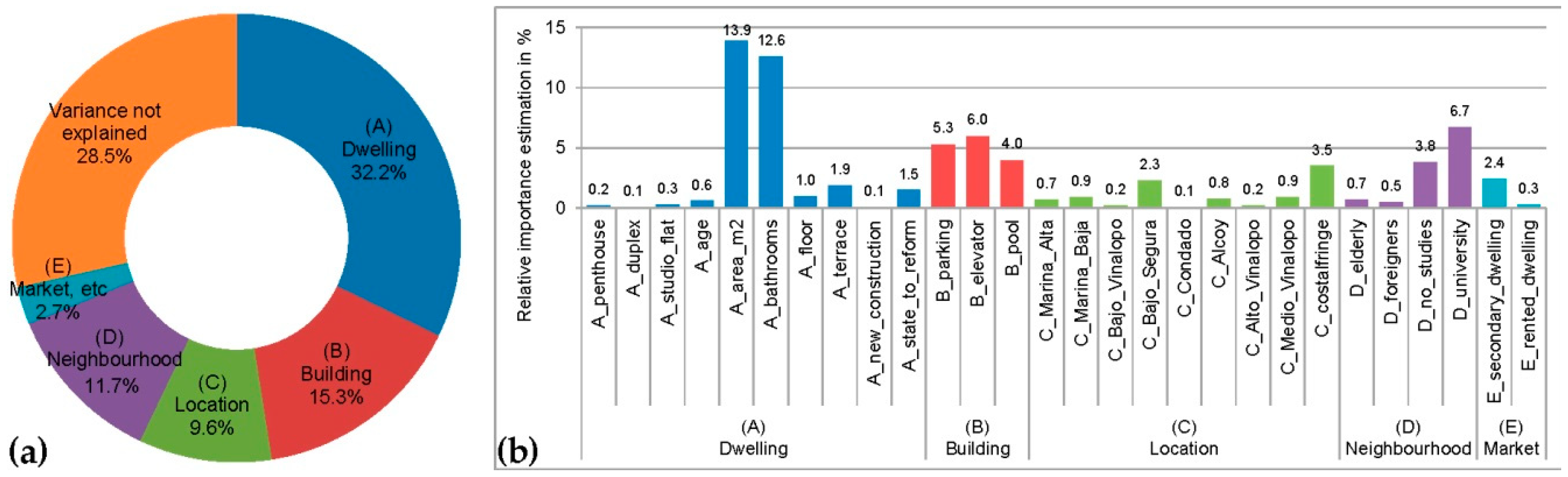
• The characteristics of the dwelling and the building have great importance in determining the price, followed by the characteristics of the neighbourhood and the location.
• Characteristics of dwellings and buildings, such as the surface area, age, housing typology (duplex, penthouse, or studio flat), the availability of garage slot or an elevator, have different effects on the price depending on the quantile.
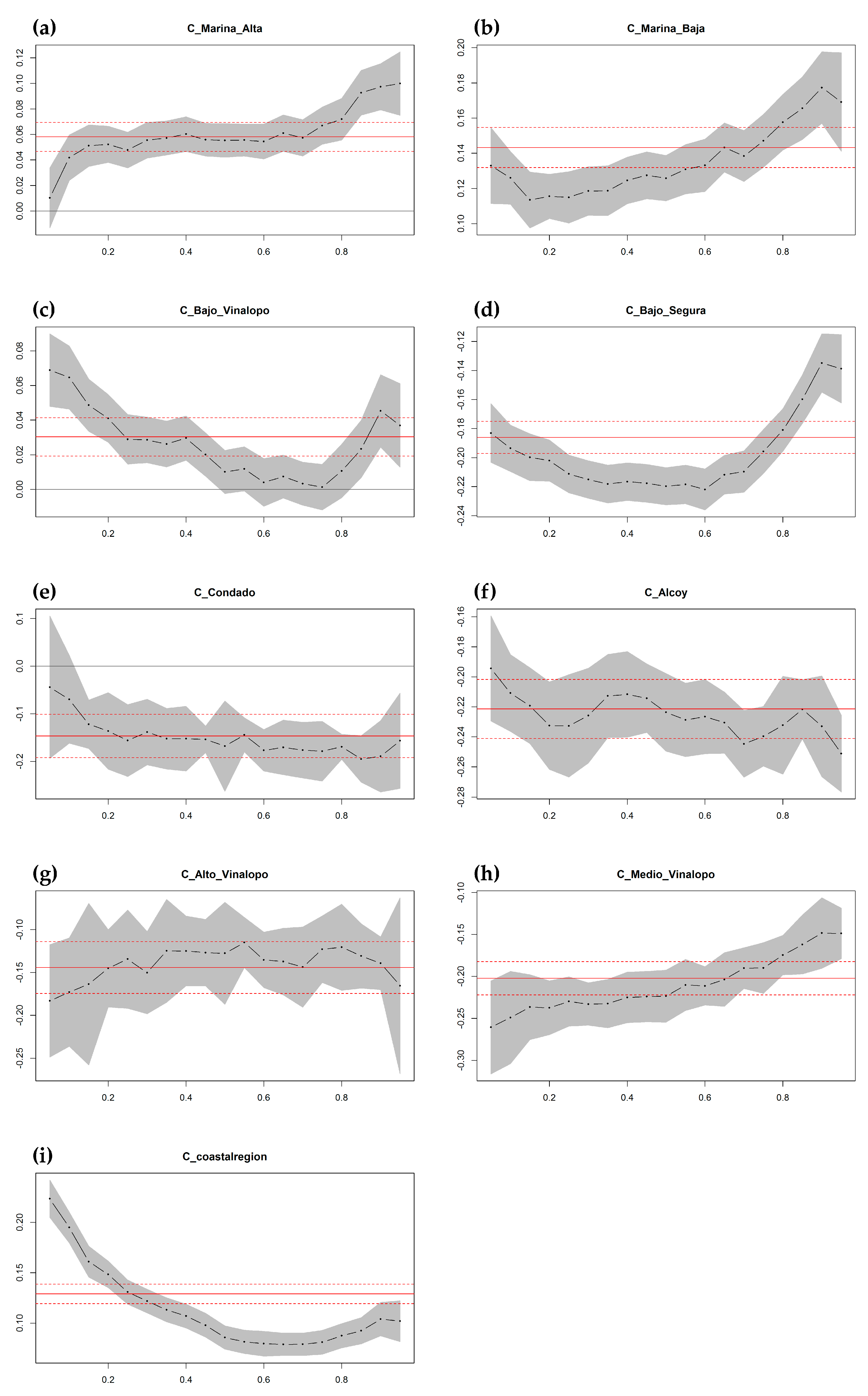
• Location characteristics also show that there are two distinct markets, the coast and the inland areas.
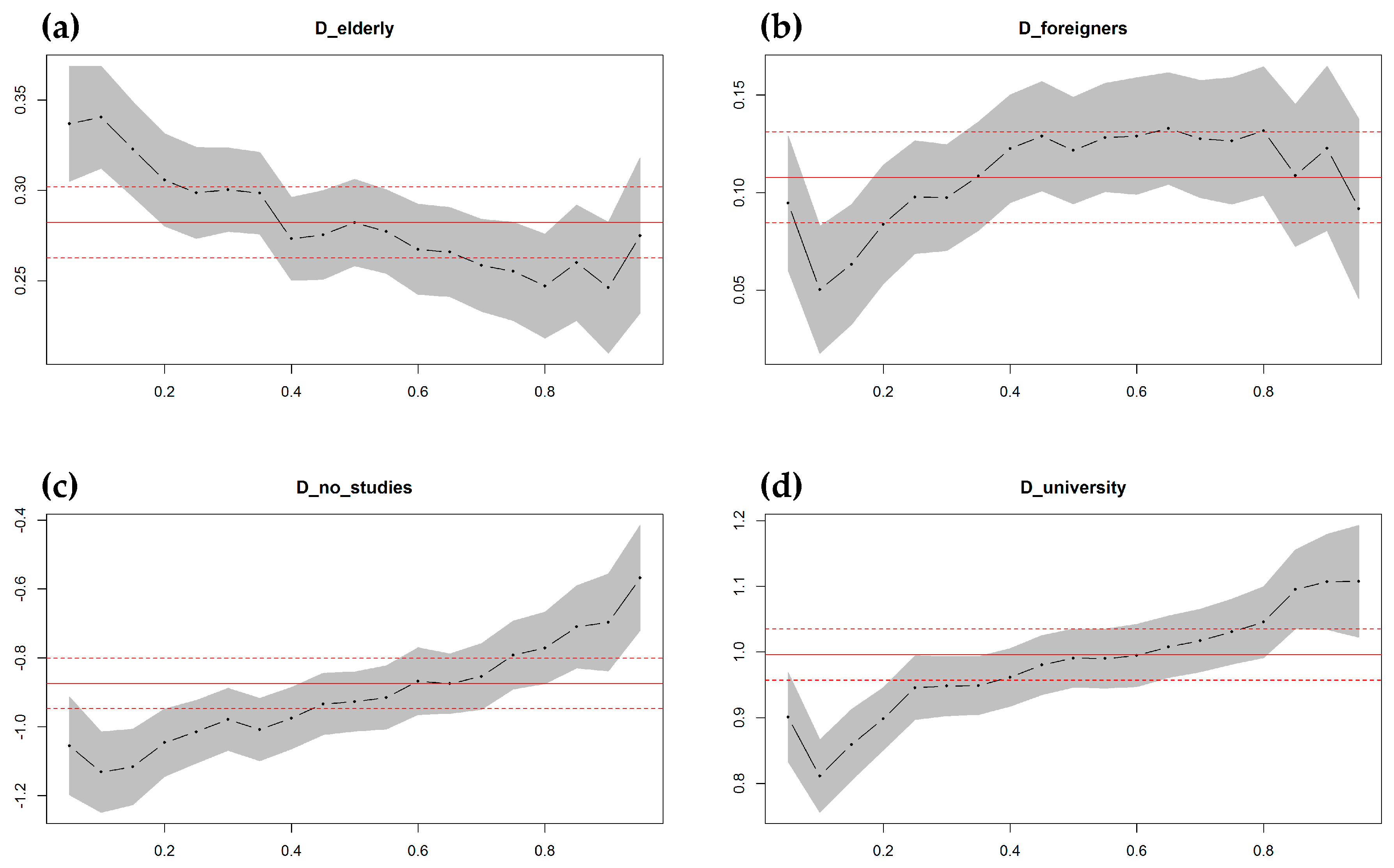
• Neighbourhood characteristics show that certain segments of the population are willing to pay more for a home: people with university studies and foreigners. The latter are persons with sufficient economic resources; therefore, this population segment is mainly from Europe.
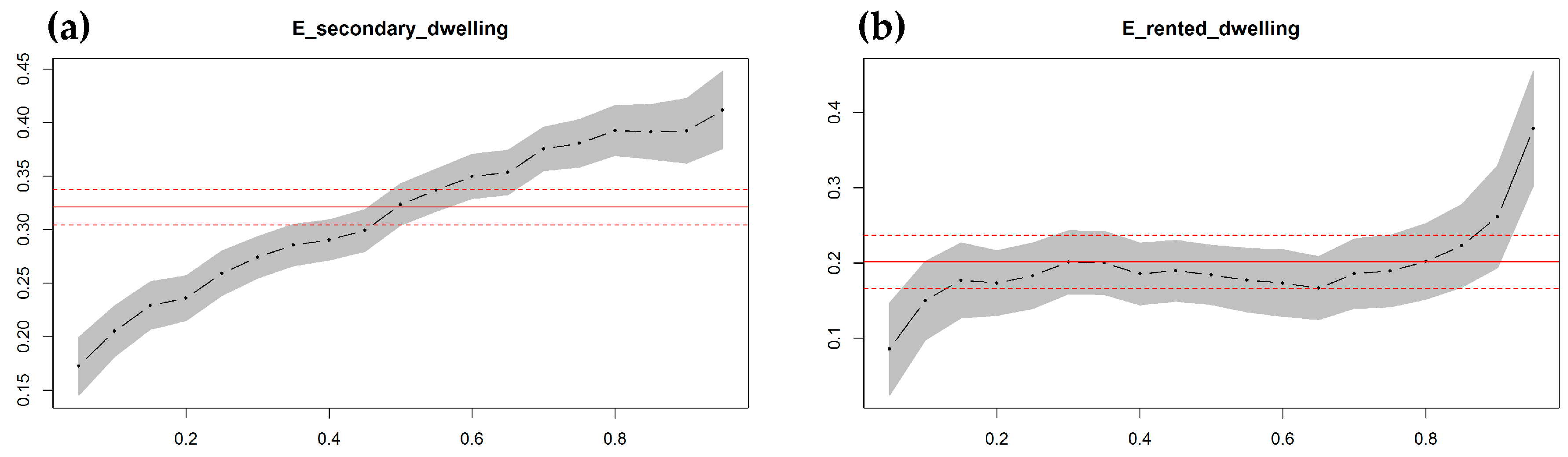
• Finally, the market characteristics suggest that, in the province of Alicante, there is an ample second residence and rental housing market, which carries a rise in the sale price of properties as a consequence.

References

1. INE, Instituto Nacional de Estadística. Encuesta de condiciones de vida: Hogares por régimen de tenencia de la vivienda y CCAA. Available online: http://www.ine.es/jaxiT3/Tabla.htm?t=4566&L=0 (accessed on 1 October 2018).
2. Taltavull de la Paz, P. Construcción y vivienda en España, 1965–1995: Dos modelos de comportamiento del mercado inmobiliario. Ph.D. Thesis, Universidad de Alicante, Facultad de Ciencias Económicas, Alicante, Spain, 1996. Available online: http://hdl.handle.net/10045/4074 (accessed on 6 March 2018).
3. Keynes, J.M. Teoría general de la ocupación, el interés y el dinero; Fondo de Cultura Económica: México, Mexico, 1943; p. 356. ISBN 978-968-16-6841-9. [Google Scholar]
4. Ministerio de Fomento. Transacciones inmobiliarias (compraventa). Available online: https://www.fomento.gob.es/be2/?nivel=2&orden=34000000 (accessed on 15 August 2018).
5. Sirmans, G.S.; Macpherson, D.A.; Zietz, E.N. The composition of hedonic pricing models. J. Real Estate Lit. 2005, 13, 3–43. Available online: http://aresjournals.org/doi/abs/10.5555/reli.13.1.j03673877172w0w2 (accessed on 9 June 2018).
6. Court, A.T. Hedonic price indexes with automotive examples. In The Dinamics of Automovile Demand; General Motors Corporation: New York, NY, USA, 1939; pp. 99–117. [Google Scholar]
7. Lancaster, K.J. A new approach to consumer theory. J. Political Econ. 1966, 74, 132–157. [Google Scholar] [CrossRef]
8. Ridker, R.G.; Henning, J.A. The determinants of residential property values with special reference to air pollution. Rev. Econ. Stat. 1967, 49, 246–257. [Google Scholar] [CrossRef]
9. Rosen, S. Hedonic prices and implicit markets: Product differentiation in pure competition. J. Political Econ. 1974, 82, 34–55. [Google Scholar] [CrossRef]
10. Smith, L.B.; Rosen, K.T.; Fallis, G. Recent developments in economic models of housing markets. J. Econ. Lit. 1988, 26, 29–64. [Google Scholar]
11. Brounen, D.; Kok, N. On the economics of energy labels in the housing market. J. Environ. Econ. Manag. 2011, 62, 166–179. [Google Scholar] [CrossRef] [Green Version]
12. Igbinosa, S.O. Determinants of Residential Property Value in Nigeria—A Neural Network Approach. Int. Multidiscip. J. Ethiop. 2011, 5, 152–168. [Google Scholar] [CrossRef]
13. Selím, S. Determinants of House Prices in Turkey: A Hedonic Regression Model. Doğuş Üniversitesi Dergisi 2008, 9, 65–76. Available online: http://journal.dogus.edu.tr/index.php/duj/article/view/80 (accessed on 3 August 2018).
14. Galvis, L.A.; Carrillo, B. Un índice de precios espacial para la vivienda urbana en colombia: Una aplicación con métodos de emparejamiento. Revista de Economía del Rosario 2013, 16, 25–59. Available online: http://www.urosario.edu.co/economia/documentos/v16_n1Galvis_Carrillo/ (accessed on 9 October 2018).
15. Chasco Yrigoyen, C.; Sánchez Reyes, B. Externalidades ambientales y precio de la vivienda en Madrid: Un análisis con regresión cuantílica espacial. Revista Galega de Economía 2012, 21, 1–21. Available online: http://www.usc.es/econo/RGE/Vol21_2/castelan/bt4c.pdf (accessed on 9 October 2018).
16. Ferreira Vaz, A.J. La dimensión de la subjetividad en la formación del valor inmobiliario: Aplicación del método de análisis de ecuaciones estructurales al mercado residencial de Lisboa. Doctoral thesis, Universidad Politécnica de Madrid, Madrid, Spain, 2013. Available online: http://oa.upm.es/15577/ (accessed on 11 April 2018).
17. Hyland, M.; Lyons, R.C.; Lyons, S. The value of domestic building energy efficiency—Evidence from Ireland. Energy Econ. 2013, 40, 943–952. [Google Scholar] [CrossRef]
18. Yayar, R.; Demir, D. Hedonic estimation of housing market prices in Turkey. Erciyes Univ. J. Fac. Econ. Adm. Sci. 2014, 0, 67–82. [Google Scholar] [CrossRef]
19. Fuerst, F.; McAllister, P.; Nanda, A.; Wyatt, P. Energy performance ratings and house prices in Wales: An empirical study. Energy Policy 2016, 92, 20–33. [Google Scholar] [CrossRef]
20. Zahirovich-Herbert, V.; Gibler, K.M. The effect of new residential construction on housing prices. J. Hous. Econ. 2014, 26, 1–18. [Google Scholar] [CrossRef]
21. Chasco Yrigoyen, C.; Gallo, J.L. The impact of objective and subjective measures of air quality and noise on house prices: A multilevel approach for downtown Madrid. Econ. Geogr. 2013, 89, 127–148. [Google Scholar] [CrossRef]
22. Fernández Durán, L. Análisis del impacto de los aspectos relativos a la localización en el precio de la vivienda a través de técnicas de soft computing. Una aplicación a la ciudad de Valencia. Doctoral thesis, Universidad Politécnica de Valencia, Valencia, Spain, 2016. Available online: http://hdl.handle.net/10251/63253 (accessed on 15 February 2018).
23. Baudry, M.; Guengant, A.; Larribeau, S.; Leprince, M. Formation des prix immobiliers et consentements à payer pour une amélioration de l’environnement urbain: l’exemple rennais. Revue d’Économie Régionale & Urbaine 2009, 2, 369–411. [Google Scholar] [CrossRef]
24. García Pozo, A. Determinantes del precio de la vivienda usada en málaga una aplicación de la metodología hedónica. Revista de estudios regionales 2008, 82, 135–158. Available online: http://www.revistaestudiosregionales.com/documentos/articulos/pdf1043.pdf (accessed on 6 March 2018).
25. Humaran Nahed, I.; Roca Cladera, J. Hacia una medida integrada del factor de localización en la valoración residencial: El caso de Mazatlán. ACE: Arquitectura, Ciudad y Entorno 2010, 13, 185–218. [Google Scholar] [CrossRef]
26. Sagner, A. Determinantes del precio de viviendas en la región metropolitana de Chile. El Trimestre Económico 2011, 78, 813–839. [Google Scholar] [CrossRef]
27. Bohl, M.T.; Michels, W.; Oelgemöller, J. Determinanten von Wohnimmobilienpreisen: Das Beispiel der Stadt Münster. Jahrbuch für Regionalwissenschaft 2012, 32, 193–208. [Google Scholar] [CrossRef] [Green Version]
28. Brandt, S.; Maennig, W. The impact of rail access on condominium prices in Hamburg. Transportation 2012, 39, 997–1017. [Google Scholar] [CrossRef]
29. Nicodemo, C.; Raya, J.M. Change in the distribution of house prices across Spanish cities. Reg. Sci. Urban Econ. 2012, 42, 739–748. [Google Scholar] [CrossRef] [Green Version]
30. Bauer, T.K.; Feuerschütte, S.; Kiefer, M.; an de Meulen, P.; Micheli, M.; Schmidt, T.; Wilke, L.-H. Ein hedonischer Immobilienpreisindex auf Basis von Internetdaten: 2007–2011. AStA Wirtschafts- und Sozialstatistisches Archiv 2013, 7, 5–30. [Google Scholar] [CrossRef] [Green Version]
31. Kaya, A.; Atan, M. Determination of the factors that affect house prices in Turkey by using Hedonic Pricing Model. J. Bus. Econ. Financ. 2014, 3, 313–327. Available online: http://dergipark.gov.tr/jbef/issue/32410/360453 (accessed on 3 August 2018).
32. Wen, H.; Bu, X.; Qin, Z. Spatial effect of lake landscape on housing price: A case study of the West Lake in Hangzhou, China. Habitat Int. 2014, 44, 31–40. [Google Scholar] [CrossRef]
33. Alkan, L. Housing market differentiation: The cases of Yenimahalle and Çankaya in Ankara. Int. J. Strateg. Prop. Manag. 2015, 19, 13–26. [Google Scholar] [CrossRef]
34. Fitch Osuna, J.M. Sistema de valuación masiva de inmuebles para tasaciones. Contexto. Revista de la Facultad de Arquitectura de la Universidad Autónoma de Nuevo León 2016, X, 51–63. Available online: http://www.redalyc.org/articulo.oa?id=353647474005 (accessed on 25 June 2018).
35. Van Dijk, D.; Siber, R.; Brouwer, R.; Logar, I.; Sanadgol, D. Valuing water resources in Switzerland using a hedonic price model. Water Resour. Res. 2016, 52, 3510–3526. [Google Scholar] [CrossRef]
36. Zambrano Monserrate, M.A. Formación de los precios de alquiler de viviendas en Machala (Ecuador): Análisis mediante el método de precios hedónicos. Cuadernos de Economía 2016, 39, 12–22. [Google Scholar] [CrossRef]
37. Keskin, B.; Watkins, C. Defining spatial housing submarkets: Exploring the case for expert delineated boundaries. Urban Stud. 2017, 54, 1446–1462. [Google Scholar] [CrossRef]
38. Lara Pulido, J.A.; Estrada Díaz, G.; Zentella Gómez, J.C.; Guevara Sanginés, A. Los costos de la expansión urbana: Aproximación a partir de un modelo de precios hedónicos en la Zona Metropolitana del Valle de México. Estudios demográficos y urbanos 2017, 32, 37–63. [Google Scholar] [CrossRef]
39. Park, J.; Lee, D.; Park, C.; Kim, H.; Jung, T.; Kim, S. Park accessibility impacts housing prices in Seoul. Sustainability 2017, 9, 185. [Google Scholar] [CrossRef]
40. Wen, H.; Xiao, Y.; Zhang, L. School district, education quality, and housing price: Evidence from a natural experiment in Hangzhou, China. Cities 2017, 66, 72–80. [Google Scholar] [CrossRef]
41. Xiao, Y.; Chen, X.; Li, Q.; Yu, X.; Chen, J.; Guo, J. Exploring Determinants of Housing Prices in Beijing: An Enhanced Hedonic Regression with Open Access POI Data. ISPRS Int. J. Geo-Inf. 2017, 6, 358. [Google Scholar] [CrossRef]
42. Li, R.; Li, H. Have housing prices gone with the smelly wind? Big data analysis on landfill in Hong Kong. Sustainability 2018, 10, 341. [Google Scholar] [CrossRef]
43. Lama Santos, F.A.d. Determinación de las cualidades de valor en la valoración de bienes inmuebles. La influencia del nivel socioeconómico en la valoración de la vivienda. Ph.D. Thesis, Universidad Politécnica de Valencia, Valencia, Spain, 2017. Available online: http://hdl.handle.net/10251/90526 (accessed on 6 March 2018).
44. Landajo, M.; Bilbao, C.; Bilbao, A. Nonparametric neural network modeling of hedonic prices in the housing market. Empir. Econ. 2012, 42, 987–1009. [Google Scholar] [CrossRef]
45. Núñez Tabales, J.M.; Caridad y Ocerin, J.M.; Ceular Villamandos, N.; Rey Carmona, F.J. Obtención de precios implícitos para atributos determinantes en la valoración de una vivienda. Revista Internacional Administración Finanzas 2012, 5, 41–54. Available online: https://www.theibfr.com/download/riaf/2012-riaf/riaf-v5n3-2012/RIAF-V5N3-2012-3.pdf (accessed on 11 April 2018).
46. Núñez Tabales, J.M.; Caridad y Ocerin, J.M.; Rey Carmona, F.J. Artificial Neural Networks for predicting real estate prices. Revista de métodos cuantitativos para la economía y la empresa 2013, 15, 29–44. Available online: http://hdl.handle.net/10433/363 (accessed on 11 April 2018).
47. Wen, H.; Xiao, Y.; Zhang, L. Spatial effect of river landscape on housing price: An empirical study on the Grand Canal in Hangzhou, China. Habitat Int. 2017, 63, 34–44. [Google Scholar] [CrossRef]
48. Stetler, K.M.; Venn, T.J.; Calkin, D.E. The effects of wildfire and environmental amenities on property values in northwest Montana, USA. Ecol. Econ. 2010, 69, 2233–2243. [Google Scholar] [CrossRef]
49. Duque, J.C.; Velásquez, H.; Agudelo, J. Infraestructura pública y precios de vivienda: Una aplicación de regresión geográficamente ponderada en el contexto de precios hedónicos. Ecos de Economía 2011, 15, 95–122. Available online: http://publicaciones.eafit.edu.co/index.php/ecos-economia/article/view/480 (accessed on 27 July 2018).
50. Moreno Murrieta, R.E.; Alvarado Lagunas, E. El entorno social y su impacto en el precio de la vivienda: Un análisis de precios hedónicos en el Área Metropolitana de Monterrey. Trayectorias. Revista de ciencias sociales 2011, 14, 131–147. Available online: http://trayectorias.uanl.mx/33y34/pdf/7_ramsas_elias.pdf (accessed on 6 March 2018).
51. Fernández Durán, L.; Llorca Ponce, A.; Valero Cubas, S.; Botti Navarro, V.J. Incidencia de la localización en el precio de la vivienda a través de un modelo de red neuronal artificial. Una aplicación a la ciudad de Valencia. Catastro 2012, 74, 7–25. Available online: http://www.catastro.meh.es/documentos/publicaciones/ct/ct74/1.pdf (accessed on 27 July 2018).
52. McGreal, W.S.; Taltavull de la Paz, P. Implicit house prices: Variation over time and space in Spain. Urban Stud. 2013, 50, 2024–2043. [Google Scholar] [CrossRef]
53. Wen, H.; Goodman, A.C. Relationship between urban land price and housing price: Evidence from 21 provincial capitals in China. Habitat Int. 2013, 40, 9–17. [Google Scholar] [CrossRef]
54. Rey Carmona, F.J. Alternativas determinantes en valoración de inmuebles urbanos. Ph.D. Thesis, Universidad de Cordoba, Andalusia, Spain, 2014. Available online: http://hdl.handle.net/10396/12473 (accessed on 11 April 2018).
55. Quispe Villafuerte, A. Una aplicación del modelo de precios hedónicos al mercado de viviendas de Lima Metropolitana. Revista de Economía y Derecho 2012, 9, 85–121. Available online: https://revistas.upc.edu.pe/index.php/economia/article/view/161 (accessed on 9 October 2018).
56. De Ayala, A.; Galarraga, I.; Spadaro, J.V. The price of energy efficiency in the Spanish housing market. Energy Policy 2016, 94, 16–24. [Google Scholar] [CrossRef]
57. Marmolejo Duarte, C. La incidencia de la calificación energética sobre los valores residenciales: Un análisis para el mercado plurifamiliar en Barcelona. Informes de la Construcción 2016, 68, e156. [Google Scholar] [CrossRef]
58. Núñez Tabales, J.M.; Rey Carmona, F.J.; Caridad y Ocerin, J.M. Artificial Intelligence (AI) techniques to analyze the determinants attributes in housing prices. Intel. Artif. 2016, 19, 23–38. [Google Scholar] [CrossRef]
59. Casas del Rosal, J.C. Métodos de valoración urbana. Ph.D. Thesis, Universidad de Córdoba, Andalusia, Spain, 2017. Available online: http://hdl.handle.net/10396/15417 (accessed on 11 April 2018).
60. Zhang, L.; Yi, Y. Quantile house price indices in Beijing. Reg. Sci. Urban Econ. 2017, 63, 85–96. [Google Scholar] [CrossRef]
61. Cebula, R.J. The hedonic pricing model applied to the housing market of the city of Savannah and its Savannah historic Landmark district. Rev. Reg. Stud. 2009, 39, 9–22. Available online: http://journal.srsa.org/ojs/index.php/RRS/article/view/182 (accessed on 3 August 2018).
62. Ezebilo, E. Evaluation of House Rent Prices and Their Affordability in Port Moresby, Papua New Guinea. Buildings 2017, 7, 114. [Google Scholar] [CrossRef]
63. Liu, J.-G.; Zhang, X.-L.; Wu, W.-P. Application of fuzzy neural network for real estate prediction. In Advances in Neural Networks—ISNN 2006; Springer: Berlin/Heidelberg, Germany, 2006; pp. 1187–1191. [Google Scholar]
64. Bonifaci, P.; Copiello, S. Price premium for buildings energy efficiency: Empirical findings from a hedonic model. Valori e Valutazioni 2015, 14, 5–15. [Google Scholar]
65. Keskin, B.; Dunning, R.; Watkins, C. Modelling the impact of earthquake activity on real estate values: A multi-level approach. J. Eur. Real Estate Res. 2017, 10, 73–90. [Google Scholar] [CrossRef]
66. Marmolejo Duarte, C. La incidencia de la percepción del ruido ambiental sobre la formación espacial de los valores residenciales: Un análisis para barcelona. Revista de la Construcción 2008, 7, 4–19. Available online: http://www.redalyc.org/articulo.oa?id=127612580001 (accessed on 9 June 2018).
67. Agnew, K.; Lyons, R.C. The impact of employment on housing prices: Detailed evidence from FDI in Ireland. Reg. Sci. Urban Econ. 2018, 70, 174–189. [Google Scholar] [CrossRef]
68. Fitch Osuna, J.M.; Soto Canales, K.; Garza Mendiola, R. Valuación de la calidad urbano-ambiental. Una modelación hedónica: San Nicolás de los Garza, México. Estudios Demográficos y Urbanos 2013, 28, 383–428. Available online: http://www.redalyc.org/articulo.oa?id=31230010004 (accessed on 9 October 2018). [CrossRef]
69. Malpezzi, S. Hedonic Pricing Models: A Selective and Applied Review. In Housing Economics and Public Policy; O’Sullivan, T., Gibb, K., Eds.; Blackwell Science: Oxford, UK, 2003. [Google Scholar]
70. Kain, J.F.; Quigley, J.M. Housing Markets and Racial Discrimination: A Microeconomic Analysis; National Bureau of Economic Research: New York, NY, USA, 1975; p. 393. ISBN 0-870-14270-4. Available online: http://www.nber.org/books/kain75-1 (accessed on 11 April 2018).
71. Freeman, A.M.; Herriges, J.A.; Kling, C.L. The Measurement of Environmental and Resource Values, 3rd ed.; RFF Press: New York, NY, USA, 2014; p. 479. ISBN 978-0-415-50157-6. [Google Scholar]
72. Zietz, J.; Zietz, E.N.; Sirmans, G.S. Determinants of house prices: A quantile regression approach. J. Real Estate Financ. Econ. 2008, 37, 317–333. [Google Scholar] [CrossRef]
73. Koenker, R.; Bassett, G. Regression Quantiles. Econometrica 1978, 46, 33–50. [Google Scholar] [CrossRef]
74. Koenker, R. Quantile Regression; Cambridge University Press: New York, NY, USA, 2005; p. 349. ISBN 978-0-521-84573-1. [Google Scholar]
75. Buchinsky, M. Recent Advances in Quantile Regression Models: A Practical Guideline for Empirical Research. J. Hum. Resour. 1998, 33, 88–126. [Google Scholar] [CrossRef]
76. Koenker, R. R Package ‘quantreg’. 2018. Available online: https://CRAN.R-project.org/package=quantreg (accessed on 3 September 2018).
77. Barrodale, I.; Roberts, F.D.K. Solution of an overdetermined system of equations in the l1 norm [F4]. Commun. ACM 1974, 17, 319–320. [Google Scholar] [CrossRef]
78. Koenker, R.; d’Orey, V. Remark AS R92: A Remark on Algorithm AS 229: Computing Dual Regression Quantiles and Regression Rank Scores. J. R. Stat. Soc. Ser. C (Appl. Stat.) 1994, 43, 410–414. [Google Scholar] [CrossRef]
79. Koenker, R.W.; D’Orey, V. Algorithm AS 229: Computing Regression Quantiles. J. R. Stat. Soc. Ser. C (Appl. Stat.) 1987, 36, 383–393. [Google Scholar] [CrossRef]
80. Koenker, R.; Machado, J.A.F. Goodness of Fit and Related Inference Processes for Quantile Regression. J. Am. Stat. Assoc. 1999, 94, 1296–1310. [Google Scholar] [CrossRef]
81. SEC, Sede electrónica del Catastro Inmobiliario. Información alfanumérica y cartografía vectorial. Available online: https://www.sedecatastro.gob.es/ (accessed on 1 October 2018).
82. INE, Instituto Nacional de Estadística. Censo de Población y vivienda de 2011. Available online: https://www.ine.es/censos2011_datos/cen11_datos_resultados.htm (accessed on 1 October 2018).
83. Limsombunchai, V.; Gan, C.; Lee, M. House price prediction: Hedonic price model vs. Artificial neural network. Am. J. Appl. Sci. 2004, 1, 193–201. [Google Scholar] [CrossRef]
84. Shimizu, C.; Nishimura, K.G.; Watanabe, T. House prices from magazines, realtors, and the land registry. BIS Pap. 2012, 64, 29–38. Available online: https://www.bis.org/publ/bppdf/bispap64f.pdf (accessed on 9 October 2018).
85. Mora García, R.T. Modelo explicativo de las variables intervinientes en la calidad del entorno construido de las ciudades. Ph.D. Thesis, Universidad de Alicante, Alicante, Spain, 2016. Available online: http://hdl.handle.net/10045/65829 (accessed on 15 February 2018).
86. Zheng, S.; Kahn, M.E. Land and residential property markets in a booming economy: New evidence from beijing. J. Urban Econ. 2008, 63, 743–757. [Google Scholar] [CrossRef]
87. Din, A.; Hoesli, M.; Bender, A. Environmental variables and real estate prices. Urban Stud. 2001, 38, 1989–2000. [Google Scholar] [CrossRef]
88. Kleinbaum, D.; Kupper, L.; Nizam, A.; Rosenberg, E. Applied Regression Analysis and Other Multivariable Methods, 5th ed.; Cengage Learning: Boston, MA, USA, 2013; p. 1072. ISBN 978-1-285-05108-6. [Google Scholar]
89. Chatterjee, S.; Simonoff, J.S. Handbook of Regression Analysis; John Wiley & Sons Inc.: Hoboken, NJ, USA, 2013; p. 240. ISBN 978-0-470-88716-5. [Google Scholar]
90. James, G.; Witten, D.; Hastie, T.; Tibshirani, R. An Introduction to Statistical Learning: With Applications in R; Springer: New York, NY, USA, 2013; p. 426. ISBN 978-1-4614-7137-0. [Google Scholar] [CrossRef]
91. Lindeman, R.H.; Merenda, P.F.; Gold, R.Z. Introduction to Bivariate and Multivariate Analysis; Scott, Foresman and Company: Glenview, IL, USA, 1980; p. 444. ISBN 9780673150998. [Google Scholar]
92. Grömping, U. R Package ‘Relaimpo’. 2018. Available online: https://CRAN.R-project.org/package=relaimpo (accessed on 3 September 2018).
93. Grömping, U. Relative Importance for Linear Regression in R: The Package Relaimpo. J. Stat. Softw. 2006, 17, 27. Available online: https://www.jstatsoft.org/v017/i01 (accessed on 3 September 2018). [CrossRef]
94. Johnson, J.W.; Lebreton, J.M. History and use of relative importance indices in organizational research. Organ. Res. Methods 2004, 7, 238–257. [Google Scholar] [CrossRef]
95. Liao, W.-C.; Wang, X. Hedonic house prices and spatial quantile regression. J. Hous. Econ. 2012, 21, 16–27. [Google Scholar] [CrossRef]
Figure 1. (a) Number of housing transactions in the province of Alicante according to new and second-hand housing, with reference to transactions carried out in the provinces of Madrid and Barcelona; and (b) evolution of the average unit price of housing at the national level, in the province of Alicante, Madrid and Barcelona. Source: Ministry of Development [4].
Sustainability 11 00437 g001
Figure 2. (a) Map of the province of Alicante with the delimitation of the comarcas and neighbouring provinces; and (b) a map with the municipal boundary delimitation and the stain of continuous urban land.
Sustainability 11 00437 g002
Figure 3. Aerial views of the urban areas of several cities in the province of Alicante: (a) compact urban area in the centre of the city of Alicante; (b) Playa de San Juan area in the city of Alicante; (c) urban area with high-rise buildings in the city of Benidorm; and (d) urban area with dispersed construction in the municipality of Orihuela. Source: Google Maps.
Sustainability 11 00437 g003
Figure 4. (a) Thematic map by municipalities representing value ranges of the average unit price (€/m2); and (b) thematic map by municipalities representing the number of analysed houses. Drawn up from prices for 34,138 multi-family housing projects.
Sustainability 11 00437 g004
Figure 5. Error and goodness of fit measures using Model 5. Coefficient of determination R2, mean square error MSE and root mean squared error RMSE.
Sustainability 11 00437 g005
Figure 6. (a) Breakdown of the explanatory variance (R2) in Model 5 according to the grouping categories; and (b) relative importance of each variable from the breakdown of the explanatory variance in Model 5.
Sustainability 11 00437 g006
Figure 7. OLS and quantile regression coefficients, for the characteristics of the dwelling (Category A): (a) A_penthouse; (b) A_duplex; (c) A_studio_flat; (d) A_age; (e) A_area_m2; (f) A_bathrooms; (g) A_floor; (h) A_terrace; (i) A_new_construction; and (j) A_state_to_reform.
Sustainability 11 00437 g007
Figure 8. OLS regression and quantile regression coefficients, for the characteristics of the building (Category B): (a) Intercept; (b) B_parking; (c) B_elevator; and (d) B_pool.
Sustainability 11 00437 g008
Figure 9. OLS and quantile regression coefficients, for the characteristics of the location (Category C): (a) C_Marina_Alta; (b) C_Marina_Baja; (c) C_Bajo_Vinalopo; (d) C_Bajo_Segura; (e) C_Condado; (f) C_Alcoy; (g) C_Alto_Vinalopo; (h) C_Medio_Vinalopo; and (i) C_coastalregion.
Sustainability 11 00437 g009
Figure 10. OLS and quantile regression coefficients, for the characteristics of the neighbourhood (Category D): (a) D_elderly; (b) D_foreigners; (c) D_no_studies; and (d) D_university.
Sustainability 11 00437 g010
Figure 11. OLS and quantile regression coefficients, for the characteristics of Category E: (a) E_secondary_dwelling; and (b) E_rented_dwelling.
Sustainability 11 00437 g011