Estimating Regional Shadow Prices of CO₂ in China: A Directional Environmental Production Frontier Approach

Abstract

Shadow price of carbon dioxide (CO₂) plays a fundamental role in evaluating CO₂ abatement cost and formulating regional environmental policies. In this study, CO₂ shadow prices are estimated in 29 provinces of China from 2006 to 2015. Directional Environmental Production Frontier Function (DEPFF) measures the distance between actual production points and the effective production frontier surface, which yields the shadow prices of CO₂ emission. With the relationship between CO₂ emission and Gross Domestic Product (GDP) growth which is encapsulated in the shadow price, the provinces are classified into three groups: acceleration zone, buffer zone, and deceleration zone. The acceleration zone is characterized by a smaller emission growth driving a greater economic growth, and the provincial average price of CO₂ is 184.16 US$/ton. In the buffer zone, a significant emission increase brings about less economic growth with the average shadow price at 86.57 US$/ton. In the deceleration zone, a high growth rate of CO₂ emissions is accompanied with an economic output decrease, which implies that the shadow price of CO₂ should be negative, and the mean value is −200.7 US$/ton. As the CO₂ abatement potential differs significantly across provinces, the environmental policy and CO₂ reduction targets should be region-specific.

1. Introduction

Global warming is a severe problem confronted by the international community. Kyoto Protocol is an intergovernmental commitment signed to protect the world from climate hazards. Developed countries have promised to reduce their carbon dioxide (CO₂) emissions since 2005, and they have committed to reduce their emissions since 2012 [1]. In 2006, China accounted for 28% of global CO₂ emissions, overtaking the United States to be the world’s largest CO₂ emitter, while the United States and Europe accounted for only 14% and 10%, respectively [2]. As a responsive country, China is actively working to reduce its CO₂ emissions. In calculating the consumption of eight kinds of fossil energy, Figure 1 shows CO₂ emissions and the corresponding Gross Domestic Product (GDP) in China during 2006–2015. In 2006–2011, CO₂ emissions grew at a relative high speed of 7.3% annually, and the speed declined to 0.66% during 2012–2015. From 2005 to 2017, China reduced CO₂ emission per unit of GDP by 45% and this remarkable progress is credited to hard work and effective measurements. In the Paris Climate Agreement, China pledges that by 2030, their carbon intensity will be further reduced to 60–65% of the previous level in 2005, and then the emission will reach its peak [3]. Undoubtedly, this future task is difficult. In 2013, the National Development and Reform Commission of China committed to establishing the Emission Trading Scheme (ETS) and launched pilots in the seven districts of Beijing, Shanghai, Tianjin, Chongqing, Hubei, Guangdong, and Shenzhen. At the end of 2017, based on the pilot’s experiences, China further established a nationwide carbon ETS. While for complexity of the market construction and its far-reaching impact on the entire economy, all of the details are still uncertain now. In theory, CO₂ shadow prices of the market participants determine the equilibrium volume, price, and the participants’ benefits or loss. So further exploring CO₂ shadow prices of the nation is urgent and necessary.

This study aims to solve two problems. First, estimate CO₂ shadow prices of 29 provinces in China from 2006 to 2015 with a Directional Environmental Production Frontier Function (DEPFF) approach. Second, analyze provincial differences in relations of CO₂ emission and GDP growth, and then put forward region-specific environmental policies.

Section 2 contains a literature review, while Section 3 outlines the model that is employed to estimate CO₂ shadow prices—the (DEPFF). Section 4 presents the empirical results and discussion of typical cases of CO₂ shadow prices in China’s provinces. Section 5 concludes the study and provides some policy implications.

2. Literature Review

CO₂ shadow price can be defined as the opportunity cost of output loss when an additional unit of CO₂ is reduced under a certain technology [4], as estimated with the micro production efficiency model. Given the detailed technology and economic constraints, this type of model defines a set of production possibilities, then reduces CO₂ emissions and captures the opportunity costs. In recent years, the directional distance function (DDF) has been widely used for its not needing the generally unavailable data of input and output prices [5]. The distance function was first proposed by Shephard [6] and later extended by Chung [7] and F$\mathrm{ä}$re [8]. Environmental production technology is constructed with the production efficiency model and multiple inputs and outputs. The shadow price of undesirable output is estimated with the output marginal conversion rate which is derived from the dual relationship of distance function (DF) and revenue function. These models can be further divided into parametric and non-parametric kinds. Badau [9] established a parametric environmental production function with the pollutant as undesirable output, then measured the marginal effect of pollution with its partial derivative. Park and Lim [10] applied a distance function based on transcendental logarithm to estimate the CO₂ shadow price for thermal power plants in Korea. Wei [11] derived the shadow price of pollutants in 104 prefecture-level cities with a parameterized quadratic method based on the dual relationship of income function and directional distance function. Chen et al. [12] used the quadratic directional distance function to study the temporal and spatial evolution characteristics of CO₂ shadow prices and their differences in 30 provinces of China from 2000 to 2012. Many other studies [13,14,15,16,17,18,19] also did similar work with a parametric approach. In general, the advantage of this kind of method is the production function being differentiable everywhere and easily manipulated algebraically. But its shortcomings are also apparent. First, the estimated parameters and results may be misleading if the function and data are not correctly matched. Second, the parametric model confines the shadow price as an average result and the effect of economic individuals can’t be obtained [20].

The other kind is the non-parametric model. Shadow price is derived by constructing a production frontier with a mathematical programming technique and input-output combinations. Chen et al. [21] used the extremely efficient slacks-based measure (SBM) model to calculate the CO₂ shadow prices for 30 provinces in China. Lee et al. [22] used the non-parametric directional distance function to evaluate the shadow price and environmental efficiency of pollutants in the Korean thermal power generation industry. Choi et al. [23] applied a non-radial regression-based data envelopment analysis (DEA) model to estimate the shadow price of CO₂ emissions. Chen [24] employed both the parametric and non-parametric methods to estimate the directional environmental output distance function and measured the CO₂ shadow price for the industrial sub-sectors. Liu et al. [25] estimated the shadow price of China’s provincial CO₂ emissions based on the non-parametric distance function method and evaluated the performance. Wang et al. [26] also applied non-parametric methods to estimating CO₂ shadow prices. The non-parametric method has many advantages. First, it avoids the possible mistakes of falsely assuming the function form, and then becomes more flexible to application. Second, it is insensitive to the unit of measure and need not transform the data into dimensionless form. Finally, the weights of inputs and outputs are decided through optimization solution, which improves the objectivity standard of the estimation. Although the non-parametric method ignores the impact of random shocks on the frontier output and its results can’t be statistically tested, the random impact is averaged and greatly weakened when the samples are most abundant, and it has less effect on the overall characteristics of the examined region. Therefore, the non-parametric method is more practical for calculating the CO₂ shadow price and is used in this study.

Table 1. Summary of reference on estimating CO₂ shadow prices in China’s provinces.

Reference	Sample	Period	Model	Method	Average Shadow Price (US$/ton)
Wang et al. [26]	28 provinces	2007	DDF	Non-parametric	57.37
Liu et al. [25]	30 provinces	2005–2007	DDF	Non-parametric	206.44
Wei et al. [27]	29 provinces	1995–2007	DEA	SBM	13.77
Choi et al. [23]	30 provinces	2001–2010	DEA	SBM	5.55
Zhang et al. [15]	29 provinces	2006–2010	DDF	parametric	9.68
Du et al. [16]	30 provinces	2001–2010	DDF	parametric	157.03
He [28]	29 provinces	2000–2009	DF	parametric	12.56
Ma and Hailu [29]	30 provinces	2001–2010	DDF	parametric	271.91
Song et al. [30]	29 provinces	2005–2014	DEA	SBM	132.87

Notes: DDF, DEA, SBM and DF denote directional distance function, data envelopment analysis, slacks-based measure and distance function, respectively.

shows some studies on the CO₂ shadow price estimation of China. They are different in the choices of samples, period, and method, so the results are greatly divergent. What’s more, few articles were concerned with the regional shadow prices in perspective of the relations between CO₂ emissions and GDP growth. Illustrated analysis in typical regions is even more scarce.

This study employs the DEPFF to simulate marginal effects of the CO₂ emissions and CO₂ shadow price. Using a positive or negative sign of shadow price, the output changing with CO₂ abatement is available, which strengthens the interpretation of the results and enriches policy implications. Furthermore, three groups are identified for examining the trends of CO₂ shadow price in different regions of China, and corresponding environmental policies are proposed.

3. Materials and Methods

In this section, the concept of directional distance function was first introduced, then the DEPFF model was constructed to estimate shadow prices of CO₂.

3.1. Directional Distance Function

The directional distance function is a general form of the Shephard yield distance function and a generalized representation of the radial data envelopment analysis model. In recent years, it has been widely used in measuring the shadow price of undesirable output. DDF allows for simultaneous observation of the direction of change in desirable output and undesirable output. The decision-making unit (DMU) is only at the forefront of efficiency when the desirable output reaches the maximum and the undesirable output is the minimum. Referring to the definition by Fare [31], assuming input is $x\in R_{+}^N$, desirable output is $y\in R_{+}^U$, and undesirable output is $b\in R_{+}^V$, the production technology set $P\left(x\right)$ can be defined as follows:

$$P\left(x\right)=\left\{\left(y,b\right):xcanproduce\left(y,b\right)\right\}$$

(1)

$P\left(x\right)$ represents the set of possibilities for production. It gives the set of maximum output $y$ and minimum undesirable output $b$ by given conditions and the possible frontier boundary of environmental output. $P\left(x\right)$ also satisfies the following properties:

(1)

Desirable outputs and undesirable outputs have joint productivity. If $\left(y,b\right)\in P$ and $y=0$, it is implied that $b=0$.

(2)

Desirable outputs and undesirable outputs have joint weak disposability. If $\left(y,b\right)\in P,0\le \theta \le 1$, it is implied that $\left(\theta y,\theta b\right)\in P$.

(3)

Desirable outputs are freely disposable. If $\left(y,b\right)\in P$ and $y^{\prime }\le y$, it is implied that $\left(y^{\prime },b\right)\in P\left(y,b\right)$.

Chen and Delmas [32] recommended that undesirable outputs should be defined as strong disposability, on the grounds that some of the areas of production set that are lost due to weak disposition constraints of undesirable outputs should belong to a production set. However, if it is defined as strong disposability, its production set might be illogical. In actual production, the number of undesirable outputs cannot be increased indefinitely, and it should not exceed the maximum amount that can be produced in the production process. In terms of the possible set of production and production front, it is reasonable to define undesirable output as weak disposability.

After considering the above (1)–(3) properties, to constrain the direction of desirable and undesirable outputs, $g=\left(g_y,-g_b\right)$ and $g\ne 0$ are used as the directional vector of the directional distance function, which implies expansion of the desirable outputs and the reduction of the undesirable outputs under production technology $P\left(x\right)$, The directional environmental distance function is constructed as follows:

$$D\left(x_i^t,y_i^t,b_i^t;g{y}_i^t-g{b}_i^t\right)=\underset{\epsilon ,z}{\max }\left\{\epsilon :\left(y+\epsilon g{y}_i^t,b-\epsilon g{b}_i^t\right)\in P\left(x_i^t\right)\right\}$$

(2)

$$s.t.P^T(X^T)=\{\begin{array}{l}{\displaystyle \sum _{i=1}^I}{z}_i^t{y}_{i,u}^t\ge y_{i,u}^t,u=1,\dots ,U;\\ {\displaystyle \sum _{i=1}^I}{z}_i^t{x}_{i,n}^t\le x_{i,n}^t,n=1,\dots ,N;\\ {\displaystyle \sum _{i=1}^I}{z}_i^t{B}_{i,V}^t=b_{i,v}^t,v=1,\dots ,V;\end{array}{z}_i^t\ge 0,{\displaystyle \sum _{i=1}^I}{z}_i^t=1,i=1,\dots ,I.$$

(3)

$\epsilon$ represents the degree of efficiency that a given DMU can achieve compared to the most effective DMU on the production frontier surface. $\epsilon =0$ indicates that DMU is efficient and located on the production frontier. A higher ε indicates that the technical efficiency of the DMU is lower and located away from the frontier, which indicates that the DMU has a greater potential to reduce the undesirable output while increasing the desirable output. $\left(g{y}_i^t-g{b}_i^t\right)$ is the direction vector of the function, $\epsilon g{y}_i^t$ and $\epsilon g{b}_i^t$ respectively represent the expansion ratios of the desirable output $y$ and the undesirable output $b$ from the production frontier, $z_i$ represents the non-negative weights whose sum is 1, which illustrates that the production technology is variable returns to scale.

3.2. Directional Environmental Production Frontier Function

The DDF model gives the degree of efficiency that can be achieved between DMU $i$ and the most effective DMUs on the production frontier. Therefore, based on the DDF model, the frontier output level of DMU $i$ can be calculated by adding up all outputs to construct the directional environmental production frontier function. Defined by the reference production technology $P^T\left(X^T\right)$, the DEPFF of the DMU $i\left(x_i^t,y_i^t,b_i^t\right)$ at $\mathrm{year}t$ is:

$$F^t\left(x_i^t,y_i^t,b_i^t;g{y}_i^t-g{b}_i^t\right)=\underset{\epsilon ,z}{\max }\left(y_i^t+\epsilon y_i^t\right)$$

(4)

$$\{\begin{array}{l}{\displaystyle \sum _{i=1}^I}{z}_i^t{y}_{i,u}^t\ge (1+\epsilon )y_{i,u}^t,u=1,\dots ,U;{\displaystyle \sum _{i=1}^I}{z}_i^t{x}_{i,n}^t\le x_{i,n}^t,n=1,\dots ,N;\\ {\displaystyle \sum _{i=1}^I}{z}_i^t{b}_{i,v}^t=(1-\epsilon )b_{i,v}^t,v=1,\dots ,V;z_i^t\ge 0,{\displaystyle \sum _{i=1}^I}{z}_i^t=1,i=1,\dots ,I.\end{array}$$

(5)

DEPFF presents the corresponding frontier output under the conditions of input $x$, production technology $P\left(x\right)$, actual expected output $y$, undesirable output $b,$ and direction vector $g$. $F^{t+1}\left(x_i^{t+1}{y}_i^{t+1},b_i^{t+1}\right)$ of the DMU $i\left(x_i^{t+1},y_i^{t+1},b_i^{t+1}\right)$ at year $t+1$ under the reference production technology $P^{t+1}\left(X^{t+1}\right)$ can be obtained by changing the time to $t+1$ in the algorithm of year $t$.

3.3. Intertemporal Directional Environmental Production Frontier Function

Before deriving the shadow price, it is necessary to observe the influence of a single change of undesirable output $b$ on the production frontier surface while keeping input $x$, desirable output $y$, and directional vector $gconstant$, thereby constructing the intertemporal DEPFF of period $t$ and $t+1$. The meaning of the intertemporal DEPFF is the effect of a single change in undesirable output $b$ on frontier output while keeping some factors constant. The intertemporal DEPFF is defined as follows:

Defined by the reference production technology $P^T\left(X^T\right)$, the intertemporal DEPFF of the decision-making unit $i$ in year $t$ which uses intertemporal input-output level $\left(x^t,y^t,b^{t+1}\right)$ is:

$$F^t\left(x_i^t,y_i^t,b_i^{t+1};g{y}_i^t-g{b}_i^t\right)=\underset{\epsilon ,z}{\max }\left(y_i^t+\epsilon y_i^t\right)$$

(6)

$$\{\begin{array}{l}{\displaystyle \sum _{i=1}^I}{z}_i^t{y}_{i,u}^t\ge (1+\epsilon )y_{i,u}^t,u=1,\dots ,U;{\displaystyle \sum _{i=1}^I}{z}_i^t{x}_{i,n}^t\le x_{i,n}^t,n=1,\dots ,N;\\ {\displaystyle \sum _{i=1}^I}{z}_i^t{b}_{i,v}^t=b_{i,v}^{t+1}-\epsilon b_{i,v}^t,v=1,\dots ,V;z_i^t\ge 0,{\displaystyle \sum _{i=1}^I}{z}_i^t=1,i=1,\dots ,I.\end{array}$$

(7)

By the same method, defined by the reference production technology $P^{t+1}\left(X^{t+1}\right)$, the intertemporal DEPFF of DMU $i$ in year $t+1$ with input-output level of $\left(x^{t+1},y^{t+1},b^t\right)$ is:

$$F^{t+1}\left(x_i^{t+1},y_i^{t+1},b_i^t;g{y}_i^{t+1}-g{b}_i^{t+1}\right)=\underset{\epsilon ,z}{\max }\left(y_i^{t+1}+\epsilon y_i^{t+1}\right)$$

(8)

$$\{\begin{array}{l}{\displaystyle \sum _{i=1}^I}{z}_i^{t+1}{y}_{i,u}^{t+1}\ge (1+\epsilon )y_{i,u}^{t+1},u=1,\dots ,U;{\displaystyle \sum _{i=1}^I}{z}_i^{t+1}{x}_{i,n}^{t+1}\le x_{i,n}^{t+1},n=1,\dots ,N;\\ {\displaystyle \sum _{i=1}^I}{z}_i^{t+1}{b}_{i,v}^t=b_{i,v}^t-\epsilon b_{i,v}^{t+1},v=1,\dots ,V;z_i^{t+1}\ge 0,{\displaystyle \sum _{i=1}^I}{z}_i^{t+1}=1,i=1,\dots ,I.\end{array}$$

(9)

3.4. Marginal Effect of Undesirable Output and Shadow Price of CO₂

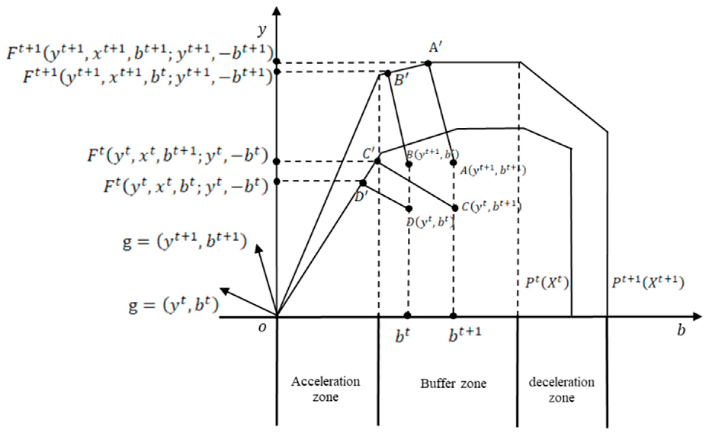
According to the definition and nature of the production technology, as shown in Figure 2, the relationship between the DEPFF and the undesirable output variable b is given as: under the production technology $P^T\left(X^T\right)$ and the direction vector $g=\left(y^t,b^t\right)$, if $b^t\le b^{t+1}$, it is implied that $F^t\left(y^t,x^t,b^t;y^t,-b^t\right)\le F^t\left(y^t,x^t,b^{t+1};y^t,-b^t\right)$. Similarly, if production technology is $P^{t+1}\left(X^{t+1}\right)$ and the direction vector is $g=\left(y^{t+1},b^{t+1}\right)$, if $b^t\le b^{t+1}$, it is implied that $F^{t+1}\left(y^{t+1},x^{t+1},b^t;y^{t+1},-b^{t+1}\right)\le F^{t+1}\left(y^{t+1},x^{t+1},b^{t+1};y^{t+1},-b^{t+1}\right)$. The difference between the decision unit $A\left(y^{t+1},b^{t+1}\right)$ and $B\left(y^{t+1},b^t\right)$, that is, the difference between producer’s frontier output $F^{t+1}\left(y^{t+1},x^{t+1},b^{t+1};y^{t+1},-b^{t+1}\right)$ and $F^{t+1}\left(y^{t+1},x^{t+1},b^t;y^{t+1},-b^{t+1}\right),$ lies in the corresponding. The undesirable output $b$ is different, which means that the frontier output will increase with an increase in $b$. Moreover, the change in $b$ in different periods leads to different growth rates for frontier output. At this point, as $b$ increases constantly, the production frontier surface will turn sharply to the lower right. The economic implication is that the increase in undesirable output $b$ will contribute to a rapid increase in frontier output for a certain period. However, if the growth of undesirable output $b$ can grow indulgently, it will not promote economic growth, but will lead to negative growth in frontier output.

Chung [7] applied a directional distance function containing undesirable outputs to the Malmquist model. The geometric mean of the Malmquist-Luenberger (ML) indices of the two periods using adjacent cross reference is used as the $ML$ index of the evaluated decision unit. The $ML$ can be decomposed into efficiency change $EC$ and technology change $TC$. According to the idea of the $ML$ index decomposition method and the relationship between the undesirable output $b$ and the DEPFF, it is also possible to use adjacent cross referencing while retaining the condition of reference technology and the input and expected output levels in the two periods. The geometric average of the change in the frontier output $F$ caused by the change in the undesirable output $b$ is used as the marginal effect of undesirable output change on frontier output:

$$MEC={\left[\frac{F^t\left(y^t,x^t,b^{t+1},y^t,-b^t\right)}{F^t\left(y^t,x^t,b^t,y^t,-b^t\right)}\times \frac{F^{t+1}\left(y^{t+1},x^{t+1},b^{t+1};y^{t+1},-b^{t+1}\right)}{F^{t+1}\left(y^{t+1},x^{t+1},b^t;y^{t+1},-b^{t+1}\right)}\right]}^{1/2}$$

(10)

$MEC$ denotes the marginal effects of the CO₂ emissions change on the frontier’s desirable output level, which means that undesirable output from $b^t$ to $b^{t+1}$ leads to changes in the frontier output from $F\left(y,x,b^t;y,-b\right)$ to $F\left(y,x,b^{t+1};y,-b\right)$ while keeping the technical structure $P$, input level $x$, and the direction vector $g$ constant. If $MEC$ is equal to 1.15, namely the marginal net effect is 15%, and indicates that the marginal contribution of CO₂ emissions leads to an increase in frontier output by 15% over the previous year. $MEC$ is equal to 0.85 and the marginal net effect is −15%, which denotes the frontier output reduced by 15% due to the change in CO₂ emissions. The shadow price of CO₂ is the change amount of frontier output caused by the change of CO₂ emission per unit. Under different reference technologies and input-output levels, CO₂ emissions have different shadow prices, which can measure the impact of emissions reduction on output. $MEC$ is the ratio of the change in the undesirable output $b^t$ to $b^{t+1}$ to the frontier output. Linking the absolute effect of marginal output with the amount of CO₂ emission change can derive the CO₂ shadow price formula:

$$S{P}_{C{O}_2}=\frac{y_{i,t-1}\times \left(ME{C}_{i,t}-1\right)}{C{O}_{2i,t}-C{O}_{2i,t-1}}$$

(11)

The shadow price of CO₂ is related to the size of the economy and the level of emissions. From the perspective of emissions reduction, a decrease in output caused by the reduction in CO₂ emissions should be as low as possible. At this time, a lower shadow price indicates that emissions reduction has had a lower impact on economic output. Conversely, the increase in output has caused an increase in CO₂ emissions as much as possible. A higher shadow price indicates that the benefits of increased CO₂ emissions are significant. This shows that the shadow price of CO₂ depends on the marginal contribution of output and the scale of CO₂ emissions. Compared with the traditional GDP per unit of CO₂ emission evaluation method, the shadow price of CO₂ strips away many factors that affect output, and it is more practical to link the changes in CO₂ emissions to the changes in frontier output. The relationship between actual CO₂ emissions and output varies regularly. Figure 2 shows that the change of undesirable output causes three variation trends in frontier output of DEPFF. Thus, it can be concluded that the provinces can be classified into three groups, based on the characteristics of CO₂ shadow price changes:

(1)

Acceleration zone—its typical feature is that even a small growth in emissions at low emission levels can contribute to greater economic growth, while shadow prices are higher. This means that reducing emissions will lead to a sharp reduction in the economy. Since the cost of cutting emissions is relatively high, CO₂ emission control should be suspended to encourage economic development.

(2)

Buffer zone—a significant emission increase brings about less economic growth, and the CO₂ shadow price is relatively low. Therefore, these regions can significantly reduce CO₂ emissions at the expense of smaller economic output. At this point, if producers still pursue economic growth through substantial increases in CO₂ emissions, the environmental cost is huge.

(3)

Deceleration zone—it is characterized by a high growth rate of CO₂ emissions accompanied with economic output decreasing, which implies that the shadow price should be negative. That means producers cannot promote economic growth by expanding CO₂ emissions. In this case, environmental regulations should be strengthened by shutting down the enterprises with high energy consumption and low efficiency. besides, the industrial structure and energy consumption structure should be optimized to promote effective emissions reduction.

3.5. Data and Variables

There are 34 provincial administrative regions in China. Hong Kong, Macau, Taiwan, Tibet, and Chongqing were excluded due to a lack of relevant data. The remaining 29 provincial regions were analyzed from 2005 to 2015. This study uses “two inputs and two outputs” as the research sample. The “two inputs” are capital stock and labor, and the “two outputs” are GDP and CO₂ emissions, of which CO₂ emissions are undesirable output. A statistical description of the input-output data is presented in

Table 2. Descriptive statistics of input-output data.

Category	Variable	Samples	Mean	Max	Min	Standard Deviation
Desirable output	GDP (billion US$)	319	133.22	648.49	5.62	116.34
Undesirable output	CO2 emissions (thousand tons)	319	373,214	1,377,266	16,396	258,755
Input	Capital stock (billion US$)	319	322.62	1451.77	17.687	267.53
	Labor force (thousand persons)	319	26,077.5	66,366	2910.4	17,337.7

, and a detailed description of each variable is provided below.

Capital stock—estimated using the perpetual inventory method. We used the approach proposed by Shan [33] to calculate the capital (constant 2000 US$). The formula is $K_t=I_t+\left(1-{\delta }_t\right)K_{t-1}$, where $K_t$ is the capital stock in year $t$, $K_{t-1}$ is the capital stock in year $t-1$, $\mathsf{\delta }$ is the capital depreciation rate (10.96%), and $I_t$ is the investment in year $t$. The related data were obtained from China Statistical Yearbook 2016 [34].

Labor—the total number of employees, collected from the China Statistical Yearbook 2016 [34] is used as the input.

GDP—the gross domestic product of each provincial region is chosen as the desirable output based on data at constant prices (constant 2000 US$), obtained from the China Statistical Yearbook 2016 [34].

CO₂ emissions—CO₂ emissions were derived from fossil fuel consumption and its conversion, since there is a lack of official statistical data on CO₂ emissions in China. This study uses the approach introduced in the Intergovernmental Panel on Climate Change (IPCC) to measure the CO₂ emissions of various provinces in China. Therefore, the formula is $b={{\displaystyle \sum }}^{\text{}}{E}_i\times NC{V}_i\times CO{F}_i\times CE{F}_i\times 44/12$, where $b$ denotes the types of various sources of energy consumption $i$, including raw coal, coke, crude oil, gasoline, diesel oil, kerosene, natural gas, and fuel oil, respectively. $NC{V}_i$ denotes the net caloric value, $CO{F}_i$ denotes CO₂ oxidation factor, $CE{F}_i$ denotes CO₂ emission factor, $44/12$ is the ratio of the molecular weight of CO₂ (44) to the atomic weight of C (12) (named the CO₂ gasification coefficient). Various sources of energy consumption $i\mathrm{and}NC{V}_i$ used in the calculations were obtained from the China Energy Statistical Yearbook 2016 [35]. $CE{F}_i$ and $CO{F}_i$ were derived from Table 1, Table 2 and

Table 3. Division of stages of CO₂ shadow prices in various provinces of China.

Zone	Provinces	Net Effect of Marginal Output of CO2 Emissions a %)	Absolute Effect of Marginal Output of CO2 Emissions b (Billion US$)	Change in CO2 Emissions (Thousand Tons)	Shadow Price of CO2 (US$/ton)
Acceleration zone	Fujian	2.95	4.388	14,473.7	303.19
	Guangxi	2.24	1.854	11,852.1	156.44
	Qinghai	4.06	0.439	3267.9	134.51
	Hainan	5.06	0.984	5960.8	165.11
	Zhejiang	1.55	3.730	14,941.3	249.65
	Sichuan	2.23	3.569	14,923.8	239.19
	Ningxia	5.14	0.578	14,110.5	40.98
Buffer zone	Beijing	0.04	0.043	165.6	265.47
	Shanxi	1.20	0.866	25,036.5	34.59
	Jilin	0.21	0.169	7096.9	23.85
	Inner Mongolia	1.82	1.684	49,069.1	34.32
	Jiangxi	1.66	1.335	10,486.3	127.36
	Jiangsu	−1.01	−3.690	−37,350.2	98.80
	Henan	0.23	0.449	20,842.9	21.54
Deceleration zone	Tianjin	−0.62	−0.546	7601.7	−71.87
	Shanxi	−0.29	−0.223	31,749	−7.03
	Hebei	−2.01	−3.697	31,618	−116.96
	Liaoning	−1.66	−3.049	20,383.7	−149.62
	Shanghai	−2.57	−4.395	3805.4	−1154.99
	Shandong	−1.66	−5.833	65,073.6	−89.64
	Heilongjiang	−1.36	−1.529	11,707.3	−130.67
	Anhui	−1.72	−1.950	20,365.5	−95.76
	Guizhou	−4.34	−1.702	10,092.2	−168.72
	Gansu	−3.27	−1.245	8040.5	−154.89
	Guangdong	−0.55	−2.377	23,668.6	−100.44
	Hunan	−0.48	−0.658	9453	−69.69
	Hubei	−0.87	−1.190	11,962.8	−99.52
	Yunnan	−1.84	−1.278	2698.5	−473.67
	Xinjiang	−9.34	−4.378	34,496.4	−126.93

Notes: a = marginal effects of the CO₂ emissions (MEC)-1; b = gross domestic product (GDP)×(MEC-1).

and Table 1, Table 2 and Table 3 and

Table 4. Two-factor analysis of variance for significant test.

Source	Sum of Squares	Degree of Freedom	Mean Squares	F	p-Value	F-Crit
Columns	362,735.8	2	181,367.9	6.1	0.0052	3.245
Rows	587	1	587	0.02	0.889	4.091
Interaction	378,747.1	2	174,373.5	5.86	0.0062	3.245
Error	1,070,398.4	36	29,733.3
Total	1,782,468.3	41

of the Energy Volume II of the national greenhouse gas inventory guide published by the IPCC [36].

4. Results and Discussion

In this section, regional classification of three groups based on shadow prices and time series analysis are presented. The three groups are divided with the net effect of marginal output when the CO₂ emissions changing in provinces of China from 2006 to 2015.

4.1. Regional Classification of Three Groups Based on Shadow Prices

CO₂ shadow price change can be divided into three groups—acceleration zone, buffer zone, and deceleration zone. Figure 3 presents the provincial data of population, per capita GDP, and the share of industry in GDP, which was obtained from the China Statistical Yearbook [34]. Figure 4 shows the provincial data of CO₂ emissions and GDP. Table 3 presents the classification of zone and the detailed values of marginal effect, change of CO₂ emissions, and shadow price. In order to ensure the significance of classification, two-factor analysis of variance was used for statistical verification. Table 4 shows the results of the analysis of variance, “Columns” refers to the acceleration zone, buffer zone and deceleration zone. “Rows” refers to the net effect of marginal output of CO₂ emissions and Shadow price of CO₂. Due to $F_C=6.1>F-crit=3.245,P-value=0.0052<\alpha =0.05$, it is implied that the classification of the three zones passed the significance test. This study calculates the average shadow price of CO₂ in China to be 157.14 US$/ton. Compared with the average shadow price measured in the other studies of Table 1, due to different methods and examining periods, the result of this study is larger than [15,23,26,27,28,30], but smaller than [25,29].

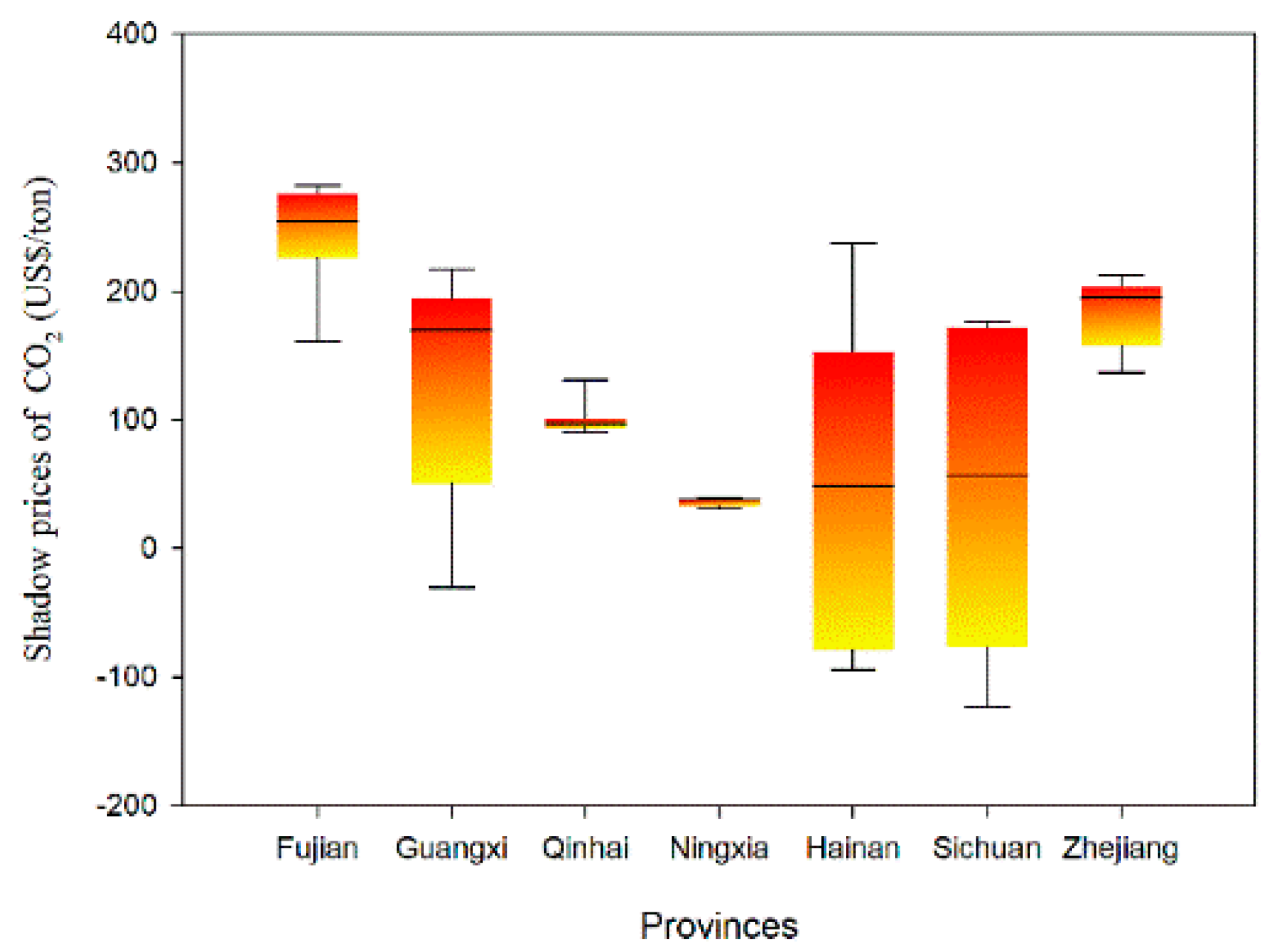
4.1.1. Analysis of the Characteristics of Shadow Prices in the “Acceleration Zone”

A typical feature of the acceleration zone is that a smaller emission increase at a low emission level can promote greater economic output growth, while the shadow price is higher. A common characteristic of Fujian, Guangxi, Qinghai, Ningxia, Zhejiang, Hainan, and Sichuan provinces are that with a substantial increase in CO₂ emissions, the net effect of its marginal output increased rapidly by more than 2%. Among these provinces, Fujian’s annual CO₂ emission growth rate of 7.64% led to an increase of 2.95% in economic output, and the absolute effect of marginal output reached an annual average of 4.388 billion US$. Ningxia has an average annual economic output value of 0.5 billion US$. Figure 5 presents the box plot distribution of the annual shadow price of the provinces in the acceleration zone from 2006 to 2015, and indicates that shadow prices are relatively high each year. To better visualize the interannual variability of provincial shadow prices,

Table 5. Shadow price analysis of Ningxia Province from 2006 to 2015.

	2006	2007	2008	2009	2010	2011	2012	2013	2014	2015
Per capita GDP (US$/person)	1236.8	1423.46	1829.097	2368.694	2630.580	3244.588	3991.471	4396.260	4785.103	5053.391
Share of industry in GDP (%)	8.17	7.88	8.18	8.52	8.76	9.43	9.40	9.88	10.65	10.96
CO2 emissions (thousand tons)	83,155	94,039.4	104,010.7	114,407.9	135,352.3	180,396.6	193,570.9	205,776.5	209,644.6	216,982.6
Growth rate of CO2 emissions (%)	9.59	13.09	10.60	10.00	18.31	33.28	7.30	6.31	1.88	3.50
GDP (billion US$)	6.760	7.619	8.579	9.600	10.896	12.217	13.619	14.954	16.150	17.442
Net effect of marginal output of CO2 emissions a (%)	4.56	6.14	5.03	4.74	8.24	13.80	3.34	2.88	0.91	1.72
Absolute effect of marginal output of CO2 emissions b (billion US$)	0.274	0.415	0.384	0.407	0.791	1.503	0.408	0.392	0.136	0.278
Change in CO2 emissions (thousand tons)	7277.8	10,884.3	9971.3	10,397.2	20,944.5	45,044.3	13,174.3	12,205.7	3868.1	7337.9
Shadow price of CO2 (US$/ton)	37.66	38.16	38.48	39.12	37.76	33.89	30.95	32.18	35.23	37.86

Notes^{: a} = MEC-1; ^b = GDP×(MEC-1).

displays the empirical data of Ningxia province to demonstrate the relationship between CO₂ emissions, economic growth, and shadow prices.

In 2006, Ningxia’s CO₂ emissions of 83,155 thousand tons led to a 4.56% increase in the net effect of marginal output, while the absolute effect of marginal output reached 0.274 billion US$. From 2007 to 2010, CO₂ emissions increased by 13.09, 10.60, 10.00, and 18.31%, respectively. The annual cumulative absolute effect of marginal output reached 1.2 billion US$. In 2011, the CO₂ emissions increased 33.28% compared to the previous year. At the same time, the net effect of marginal output reached a maximum of 13.5%, and its contribution value was 1.5 billion US$. From 2012 to 2015, the growth rate of CO₂ emissions has slowed but is increasing at a positive rate. The net effect of marginal output for 2012–2015 remained at a high level of 3.34, 2.88, 0.91, and 1.72%, respectively. The absolute effect of annual cumulative marginal contribution in the four years is 1.21 billion US$. Besides, the share of industry in GDP has increased year by year. These data demonstrate that Ningxia has established many energy-consuming enterprises with large CO₂ emissions through investment promotion and industrial transfer. Therefore, the increase in CO₂ emissions has also driven the province’s rapid economic development.

This signifies that provinces in the “acceleration zone” have greater room for economic growth and CO₂ emissions growth due to their lack of development or relatively abundant environmental resources. These provinces focus on driving economic growth by increasing CO₂ emissions. Increasing people’s income is the main content of development. With the construction of many infrastructures, CO₂ emissions will increase as the economy grows. Hence, emissions reduction policies can be relaxed to allow moderate growth in CO₂ emissions in these provinces to promote economic development. It is of course necessary to vigorously develop the resource-conserving and environment-friendly industries to enhance the sustainability of economic growth.

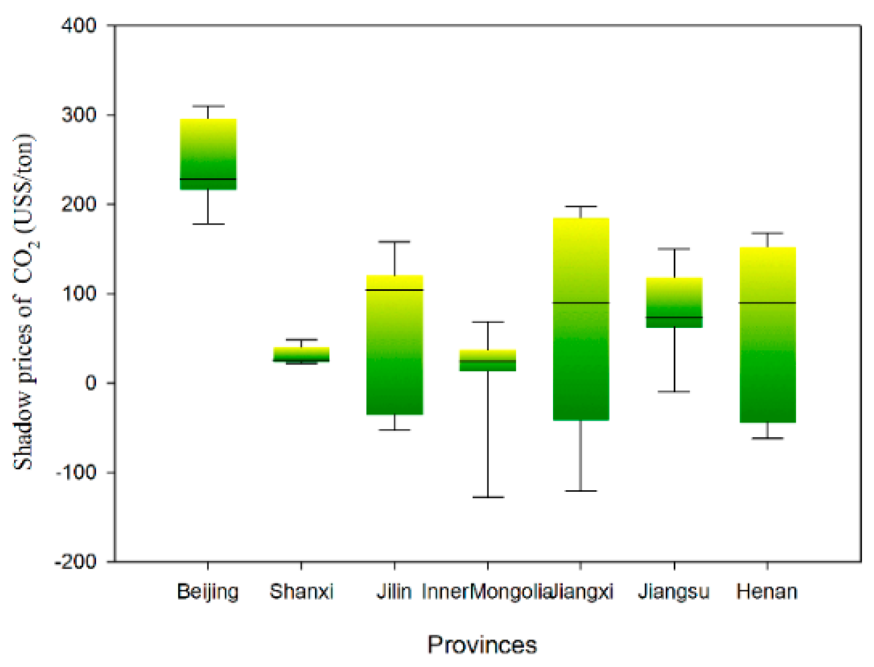
4.1.2. Analysis of the Characteristics of Shadow Prices in the “Buffer Zone”

A typical characteristic of the buffer zone is that if a substantial increase in emissions brings about less economic growth, it is implied that the economic costs of reduction emissions are falling. Beijing, Shanxi, Jilin, Inner Mongolia, Jiangsu, Jiangxi, and Henan are characterized by a continuous increase (or decrease) in CO₂ emissions, but the net effect of marginal output is not significant. The annual CO₂ emissions increased by 20,840 thousand tons in Henan province, and the net annual average marginal output was only 0.23%, while the shadow price was relatively low. In Henan Province, a substantial increase in CO₂ emissions cannot lead to rapid economic development. Jiangsu province is a major CO₂ emissions province in China. From 2006 to 2015, the annual average emissions reduction was 37,305 thousand tons. The impact on the economic marginal output fell only by 1.01% with the annual average shadow price being 817.96 US$/ton. This shows that Jiangsu province is carrying out CO₂ emission control at a small economic cost while obtaining a significant reduction in CO₂ emissions. Figure 6 shows the box plot distribution of inter-annual shadow prices from 2006 to 2015 in the buffer zone provinces. Shadow prices of provinces are lower in each successive year. To better visualize the interannual variability of provincial shadow prices, the case of Jiangsu demonstrates the relationship between CO₂ emissions, economic growth, and shadow prices.

Table 6. Shadow price analysis of Jiangsu Province from 2006 to 2015.

	2006	2007	2008	2009	2010	2011	2012	2013	2014	2015
Per capita GDP (US$/person)	2966.756	3465.041	4087.384	4833.542	5345.598	6382.875	7524.400	8256.063	9102.483	9890.075
Share of industry in GDP (%)	5.68	5.58	5.81	6.32	6.24	6.13	6.56	6.78	6.98	7.11
CO2 emissions (thousand tons)	834,587.7	840,102.5	821,452.2	804,676.5	697,719.2	624,896.2	597,774.4	579,348.7	537,564.4	491,008.5
Growth rate of CO2 emissions (%)	−3.46	0.66	−2.22	−2.04	−13.29	−10.44	−4.34	−3.08	−7.21	−8.66
GDP (billion US$)	218.21	250.73	282.57	317.61	357.95	397.32	437.45	479.45	521.16	565.46
Net effect of marginal output of CO2 emissions a (%)	−1.03	−0.93	−0.43	−0.74	−2.16	−3.12	−0.46	−0.49	0.15	−0.87
Absolute effect of marginal output of CO2 emissions b (billion US$)	−1.953	−2.029	−1.078	−2.091	−6.860	−11.168	−1.828	−2.144	0.719	−4.534
Change in CO2 emissions (thousand tons)	−29,922.9	5514.8	−18,650.3	−16,775.7	−106,957	−72,823	−27,121.8	−18,425.7	−41,784.3	−46,555.9
Shadow price of CO2 (US$/ton)	65.28	−367.99	57.80	124.64	64.14	153.35	67.38	116.33	−17.21	97.39

Notes^{: a} = MEC-1; ^b = GDP×(MEC-1).

lists the empirical data of Jiangsu province.

As a major economic province in China, Jiangsu Province is also a large CO₂ emissions province. Its economic and technical development are relatively high, and its ability to reduce emissions and allocate resources is strong. In 2006, its emissions reduction was 3.46% compared to the previous year, which caused the net effect of marginal output loss of only 1.03%. From 2008 to 2015, emissions were reduced by 2.22, 2.04, 13.29, 10.44, 4.34, 3.08, 7.21, and 8.66%, respectively, compared to the previous years. Jiangsu’s industry accounts for a lower share of GDP. Under the continuous emissions reduction measures, the marginal net effect loss to the economy remained low at −0.93, −0.43, −0.74, −2.16, −3.12, −0.46, −0.49, 0.15, and −0.87%, respectively, which indicated that the industrial structure of Jiangsu province has been adjusted along with the implementation of the emissions reduction, and the contribution of increased CO₂ emissions to economic growth is weakening, meaning that only a small loss of economic output is incurred for the achievement of emissions reduction targets.

In these provinces, the environmental costs of pursuing economic growth are beginning to rise, and the increase in CO₂ emissions does not drive rapid economic growth. CO₂ emissions should be controlled in provinces of this zone—a large reduction in CO₂ emissions will be replaced by a small output loss. Economic growth still must be ensured in the process of governance, and it calls for changes in the developing style by introducing new production technologies, improving energy efficiency and reducing fossil fuel consumption. It is possible to promote the economy and achieve the emission reduction goal by establishing a low carbon industry development model and a low carbon energy structure.

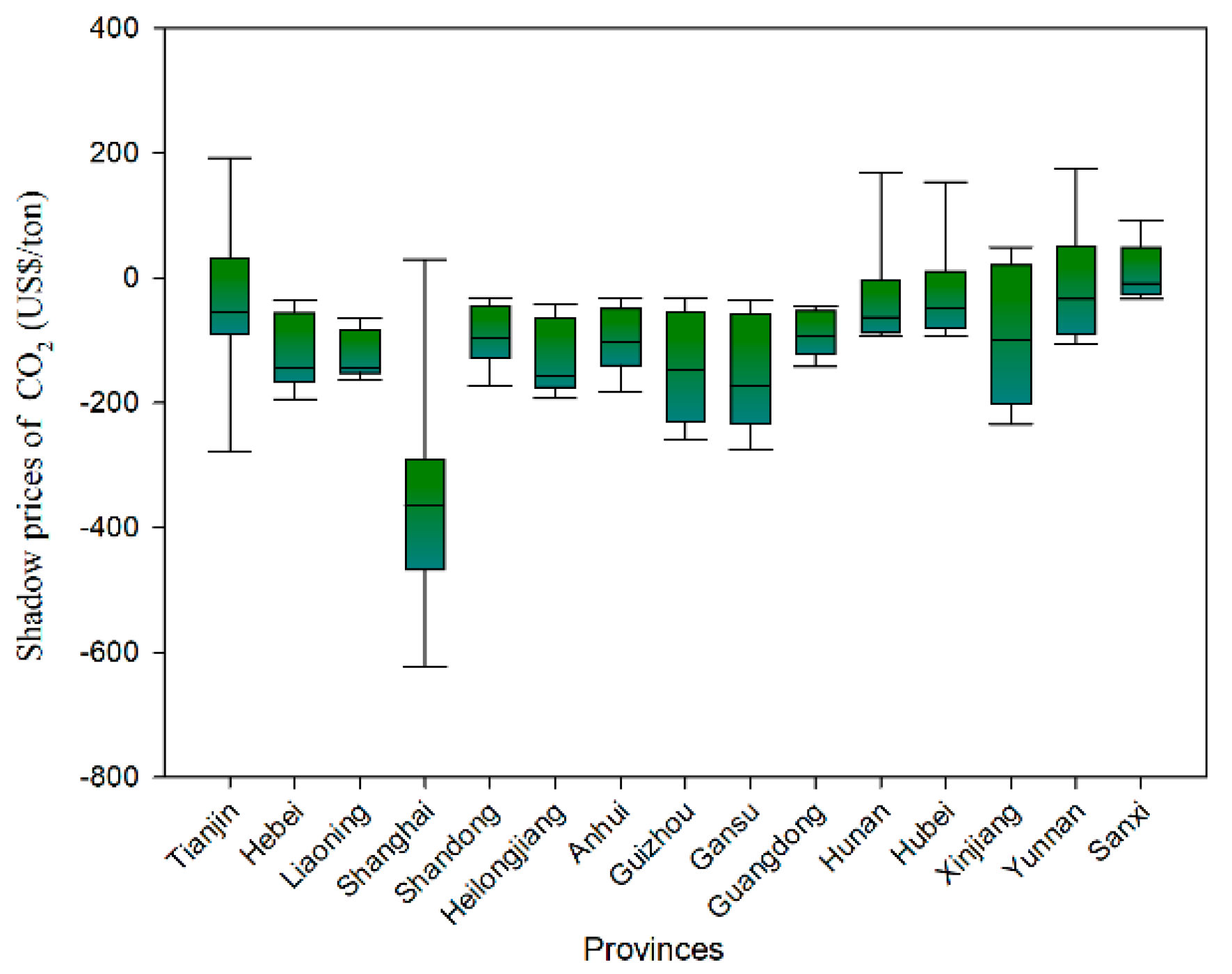
4.1.3. Analysis of the Characteristics of Shadow Prices in the “Deceleration Zone “

In the deceleration zone, both the level of economic development and CO₂ emissions are high. A substantial increase in CO₂ emissions does not lead to an increase in the marginal net effect, and the shadow price is negative. Figure 7 shows that the shadow prices in each province are basically negative. This indicates that the environmental and emissions problems in this region are serious. To better visualize the interannual variability of provincial shadow prices, Hebei is a typical case to demonstrate the relationship between CO₂ emissions, economic growth, and shadow prices.

Table 7. Shadow price analysis of Hebei Province from 2006 to 2015.

	2006	2007	2008	2009	2010	2011	2012	2013	2014	2015
Per capita GDP (US$/person)	1785.61	2040.73	2375.09	2776.62	2969.29	3462.988	4103.3	4419.21	4700.06	4829.9
Share of industry in GDP (%)	11.54	11.72	11.89	11.99	11.85	12.57	12.81	12.71	13.26	12.75
CO2 emissions (thousand tons)	646,736	705,324	737,261	786,343	846,392	957,191	970,562	971,621	924,003	91,519
Growth rate of CO2 emissions (%)	13.20	12.80	10.10	10.00	12.20	11.30	9.60	8.20	6.50	6.80
GDP (billion US$)	117.404	132.431	145.807	160.388	179.955	200.290	219.51	237.518	252.958	270.16
Net effect of marginal output of CO2 emissions a (%)	−1.62	−2.22	−1.45	−3.25	−4.84	−9.72	−1.09	−0.08	3.45	0.68
Absolute effect of marginal output of CO2 emissions b (billion US$)	−1.684	−2.606	−1.920	−4.739	−7.763	−17.492	−2.183	−0.176	8.194	1.720
Change in CO2 emissions (thousand tons)	47718	58,587	31,937.5	49,081.5	60,048.8	110,799.1	13371	1058.8	−47617	−8805.8
Shadow price of CO2 (US$/ton)	−35.29	−44.49	−60.136	−96.55	−129.28	−157.87	−163.28	−165.86	−172.09	−195.34

Notes^{: a} = MEC-1; ^b = GDP×(MEC-1).

lists the empirical data of Hebei province.

Hebei is also a large CO₂ emissions province in China. It has maintained a relatively high rate of emissions growth from 2006 to 2011—13.2, 12.8, 10.1, 10, 12.2, and 11.3%, respectively. With such a large scale of emissions, the net effect of marginal output has grown negatively. In 2011, an increase of 11.3% over the previous year’s emissions resulted in a marginal output loss of 9.72%, amounting to 17.49 billion US$. The cumulative absolute effect of marginal output decreased by 36.19 billion US$ from 2006 to 2011. In 2012 and 2013, the emissions slowed down sharply. It is worth noting that Hebei province began to reduce emissions by a total of 56,423 thousand tons, and the absolute effect of the cumulative marginal output increased by 9.92 billion US$ from 2014 to 2015. Besides, the proportion of industry in GDP is basically maintained at around 12%. It can be seen from the above that the increase in CO₂ emissions did not contribute to the economy in Hebei province from 2006 to 2013, but rather, it caused environmental damage and affected the increase in output. After 2014, the implementation of the emissions reduction policy resulted in an increase in output.

This suggests that provinces in the “deceleration zone” are already showing signs of weakness in their carbon-driven growth. It is necessary to implement structural reforms on the industrial supply side and promote the optimization and upgrading of industrial structure. In addition, it is necessary to increase industrial restructuring, environmental governance, technological innovation, and increase the share of new/alternative energy consumption. This will ensure that CO₂ emissions will be further reduced while the economy will grow. Besides, new technologies and new management models should be applied for traditional industries. The region must also take the initiative to undertake national emission reduction work.

5. Conclusions

The provincial shadow price of CO₂ in China has great differences for the regional gaps in technology and productive efficiency. This study selects 29 provinces of China as examining samples and estimates their CO₂ shadow prices during 2006–2015. The non-parametric directional distance function was applied to construct a DEPFF model, and shadow prices of CO₂ for each province are calculated with the labor and capital stock as inputs, provincial GDP, and CO₂ emissions as desirable and undesirable outputs. Trends of each province from 2006 to 2015 are also identified, and the 29 provinces and regions are finally categorized as acceleration zone, buffer zone, and deceleration zone.

Ningxia and another 6 provinces are in the acceleration zone, where the CO₂ emissions are considerable and their contributions to the economy are also significant. The shadow price of CO₂ is usually high. The average net effect of marginal output of CO₂ emissions in the acceleration zone is 2.95%, and the average shadow price is 184.16 US$/ton. If compulsory emissions reduction measures are mandated, the economy will greatly shrink, which implies a high cost of emissions reduction. Economic growth should be sustained through a lax environmental policy, and meanwhile energy efficiency improvement technologies should be developed to promote economic growth with fewer emissions.

Jiangsu and another 6 provinces are in the buffer zone, which is the transition zone from the acceleration zone. The average net effect of marginal output of CO₂ emissions for the buffer zone is 0.59%, and the average shadow price is 86.57 US$/ton. The sharp increase in CO₂ emissions has gradually diminished the contribution to the economy, and the CO₂ shadow price is relatively low. That means these regions can significantly reduce CO₂ emissions at the expense of smaller economic output. But in the long run, it is necessary to optimize and upgrade the industrial structure and seek new economic points of growth while reducing emissions.

Hebei and another 14 provinces are in the deceleration zone. The average net effect of marginal output of CO₂ emissions for the deceleration zone is −2.172%, and the average shadow price is −200.7 US$/ton. Their CO₂ emissions are considerable and the environmental resource capacity is weakening. The shadow price of CO₂ is negative in these regions, which means that the increase of CO₂ emissions is no longer contributing to economic growth, making emissions reduction urgently required. Stricter emissions control measures are recommended to be imposed in this zone, including shutting down high-energy-consuming industries.

Considering the provincial differences, emission reduction policies and targets should be region-specific in China for optimizing environmental resource allocation. At the same time, all regions must gradually promote the industry and energy consumption structure in order to avoid the excessive economic costs of CO₂ emissions reduction. Provinces and regions may also strengthen cooperation and synergy mechanisms to jointly implement China’s CO₂ abatement targets with lower costs.

References

1. Li, W. From Kyoto protocol to Paris agreement: Reform and development of international law on climate. J. Shanghai Univ. Int. Bus. Econ. 2016, 23, 62–73, 84. (In Chinese) [Google Scholar]
2. Zhao, D.X.; He, B.J.; Johnson, C.; Mou, B. Social problems of green buildings: From the humanistic needs to social acceptance. Renew. Sustain. Energy Rev. 2015, 51, 1594–1609. [Google Scholar] [CrossRef]
3. Wang, Z.X.; Hao, P.; Yao, P.Y. Non-Linear Relationship between Economic Growth and CO2 Emissions in China: An Empirical Study Based on Panel Smooth Transition Regression Models. Int. J. Environ. Res. Public Health 2017, 14, 1568. [Google Scholar] [CrossRef] [PubMed]
4. Huang, S.K.; Kuo, L.; Chou, K.-L. The applicability of marginal abatement cost approach: A comprehensive review. J. Clean. Prod. 2016, 127, 59–71. [Google Scholar] [CrossRef]
5. Wang, S.; Chu, C.; Chen, G.; Peng, Z.; Li, F. Efficiency and reduction cost of carbon emissions in China: A non-radial directional distance function method. J. Clean. Prod. 2016, 113, 624–634. [Google Scholar] [CrossRef]
6. Francis, R. Theory of Cost and Production Functions. By Shephard R. W. Princeton: Princeton University Press, 1970. Pp. xi, 308. $15.00. J. Econ. Hist. 1971, 31, 721–723. [Google Scholar]
7. Chung, Y.H.; Färe, R.; Grosskopf, S. Productivity and Undesirable Outputs: A Directional Distance Function Approach. Microeconomics 1997, 51, 229–240. [Google Scholar] [CrossRef]
8. Fare, R.; Grosskopf, S.; Lovell, C.A.K.; Yaisawarng, S. Derivation of Shadow Prices for Undesirable Outputs: A Distance Function Approach. Rev. Econ. Stat. 1993, 75, 374–380. [Google Scholar] [CrossRef]
9. Badau, F.; Fare, R.; Gopinath, M. Global resilience to climate change: Examining global economic and environmental performance resulting from a global carbon dioxide market. Resour. Energy Econ. 2016, 45, 46–64. [Google Scholar] [CrossRef]
10. Park, H.; Lim, J. Valuation of marginal CO2 abatement options for electric power plants in Korea. Energy Policy 2009, 37, 1834–1841. [Google Scholar] [CrossRef]
11. Wei, C. China’s urban CO2 marginal abatement costs and its influencing factors. World Econ. 2014, 37, 115–141. (In Chinese) [Google Scholar]
12. Chen, D.H.; Pan, Y.C.; Wu, C.Y. Research on marginal abatement cost and regional difference of carbon dioxide in China. China Popul. Resour. Environ. 2016, 26, 86–93. (In Chinese) [Google Scholar]
13. Lee, C.-Y.; Zhou, P. Directional shadow price estimation of CO2, SO2 and NOx in the United States coal power industry 1990–2010. Energy Econ. 2015, 51, 493–502. [Google Scholar] [CrossRef]
14. Tang, K.; Yang, L.; Zhang, J. Estimating the regional total factor efficiency and pollutants’ marginal abatement costs in China: A parametric approach. Appl. Energy 2016, 184, 230–240. [Google Scholar] [CrossRef]
15. Zhang, X.; Xu, Q.; Zhang, F.; Guo, Z.; Rao, R. Exploring shadow prices of carbon emissions at provincial levels in China. Ecol. Indic. 2014, 46, 407–414. [Google Scholar] [CrossRef]
16. Du, L.; Wei, C.; Cai, S. Economic development and carbon dioxide emissions in China: Provincial panel data analysis. China Econ. Rev. 2012, 23, 371–384. [Google Scholar] [CrossRef]
17. Molinos-Senante, M.; Hanley, N.; Sala-Garrido, R. Measuring the CO2 shadow price for wastewater treatment: A directional distance function approach. Appl. Energy 2015, 144, 241–249. [Google Scholar] [CrossRef]
18. Peng, J.; Yu, B.Y.; Liao, H.; Wei, Y.M. Marginal abatement costs of CO2 emissions in the thermal power sector: A regional empirical analysis from China. J. Clean. Prod. 2018, 171, 163–174. [Google Scholar] [CrossRef]
19. Matsushita, K.; Yamane, F. Pollution from the electric power sector in Japan and efficient pollution reduction. Energy Econ. 2012, 34, 1124–1130. [Google Scholar] [CrossRef]
20. Tu, Z.G. Shadow price of industrial sulfur dioxide emissions: A new analytical framework. Econ. (Q.) 2010, 9, 259–282. (In Chinese) [Google Scholar]
21. Chen, H.L.; Nie, W.L. China’s carbon emission shadow price measurement and spatial measurement. J. Ecol. 2018, 14, 1–8. (In Chinese) [Google Scholar]
22. Lee, J.D.; Park, J.B.; Kim, T.Y. Estimation of the shadow prices of pollutants with production/environment inefficiency taken into account: A nonparametric directional distance function approach. J. Environ. Manag. 2002, 64, 365–375. [Google Scholar] [CrossRef]
23. Choi, Y.; Zhang, N.; Zhou, P. Efficiency and abatement costs of energy-related CO2 emissions in China: A slacks-based efficiency measure. Appl. Energy 2012, 98, 198–208. [Google Scholar] [CrossRef]
24. Chen, S.Y. Shadow price of industrial carbon dioxide: Parametric and nonparametric methods. World Econ. 2010, 33, 93–111. (In Chinese) [Google Scholar]
25. Liu, M.L.; Zhu, L.; Fan, Y. China’s provincial carbon emission performance evaluation and marginal abatement cost estimation: Based on nonparametric distance function method. China Soft Sci. 2011, 3, 106–114. [Google Scholar]
26. Wang, Q.; Cui, Q.; Zhou, D.; Wang, S. Marginal abatement costs of carbon dioxide in China: A nonparametric analysis. Energy Procedia 2011, 5, 2316–2320. [Google Scholar] [CrossRef] [Green Version]
27. Wei, C.; Ni, J.; Du, L. Regional allocation of carbon dioxide abatement in China. China Econ. Rev. 2012, 23, 552–565. [Google Scholar] [CrossRef]
28. He, X.P. Regional differences in China’s CO2 abatement cost. Energy Policy 2015, 80, 145–152. [Google Scholar] [CrossRef]
29. Ma, C.; Hailu, A. The Marginal Abatement Cost of Carbon Emissions in China. Working Papers 2015, 37, 111–127. [Google Scholar] [CrossRef]
30. Song, J.W.; Cao, Z.J.; Zhang, K.X. China’s provincial carbon dioxide shadow price research. Price Theory Pract. 2016, 6, 76–79. (In Chinese) [Google Scholar]
31. Fare, R.; Grosskopf, S.; Weber, W.L. Shadow prices and pollution costs in US agriculture. Ecol. Econ. 2006, 56, 89–103. [Google Scholar] [CrossRef]
32. Chen, C.M.; Delmas, M.A. Measuring Eco-Inefficiency: A New Frontier Approach. Oper. Res. 2012, 60, 1064–1079. [Google Scholar] [CrossRef] [Green Version]
33. Shan, H.J. Re-estimation of China’s capital stock K: 1952–2006. Quant. Econ. Technol. Econ. Res. 2008, 25, 17–31. (In Chinese) [Google Scholar]
34. National Bureau of Statistical of China (NBSC). National Data, 2016. Available online: http://data.stats.gov.cn/index.html (accessed on 1 February 2016).
35. National Bureau of Statistical of China. China Energy Statistical Yearbook, 2016; China Statistics Press: Beijing, China, 2016. (In Chinese)
36. 2006 IPCC Guidelines for National Greenhouse Gas Inventories Volume 2 Energy. Available online: https://www.ipcc-nggip.iges.or.jp/public/2006gl/vol2.html (accessed on 1 April 2018).
Figure 1. China’s overall CO2 emissions and Gross Domestic Product (GDP) from 2006 to 2015.
Sustainability 11 00429 g001
Figure 2. Changes in undesirable output b cause three variation trends in frontier output F of directional environmental production frontier function.
Sustainability 11 00429 g002
Figure 3. Provincial data of population, per capita GDP and the share of industry in GDP.
Sustainability 11 00429 g003
Figure 4. Provincial data of CO2 emission and GDP.
Sustainability 11 00429 g004
Figure 5. Estimates of shadow prices of CO2 in the Acceleration zone from 2006 to 2015.
Sustainability 11 00429 g005
Figure 6. Estimates of shadow prices of CO2 in the Buffer zone from 2006 to 2015.
Sustainability 11 00429 g006
Figure 7. Estimates of shadow prices of CO2 in the deceleration zone from 2006 to 2015.
Sustainability 11 00429 g007