Article

Integrating a Hybrid Back Propagation Neural Network and Particle Swarm Optimization for Estimating Soil Heavy Metal Contents Using Hyperspectral Data

1
College of Natural Resources and Environment, South China Agricultural University, Guangzhou 510642, China
2
Guangdong Provincial Key Laboratory of Land Use and Consolidation, Guangzhou 510642, China
3
Institute of Agricultural Remote Sensing and Information Technology Application, Zhejiang University, Hangzhou 310058, China
4
National Engineering Research Center for Information Technology in Agriculture, Beijing 100089, China
5
Department of Geography and Environmental Resources, Southern Illinois University, Carbondale, IL 62901, USA
*
Authors to whom correspondence should be addressed.
Sustainability 2019, 11(2), 419; https://doi.org/10.3390/su11020419
Submission received: 5 November 2018 / Revised: 8 January 2019 / Accepted: 11 January 2019 / Published: 15 January 2019

Abstract

:
Soil heavy metals affect human life and the environment, and thus, it is very necessary to monitor their contents. Substantial research has been conducted to estimate and map soil heavy metals in large areas using hyperspectral data and machine learning methods (such as neural network), however, lower estimation accuracy is often obtained. In order to improve the estimation accuracy, in this study, a back propagation neural network (BPNN) was combined with the particle swarm optimization (PSO), which led to an integrated PSO-BPNN method used to estimate the contents of soil heavy metals: Cd, Hg, and As. This study was conducted in Guangdong, China, based on the soil heavy metal contents and hyperspectral data collected from 90 soil samples. The prediction accuracies from BPNN and PSO-BPNN were compared using field observations. The results showed that, 1) the sample averages of Cd, Hg, and As were 0.174 mg/kg, 0.132 mg/kg, and 9.761 mg/kg, respectively, with the corresponding maximum values of 0.570 mg/kg, 0.310 mg/kg, and 68.600 mg/kg being higher than the environment baseline values; 2) the transformed and combined spectral variables had higher correlations with the contents of the soil heavy metals than the original spectral data; 3) PSO-BPNN significantly improved the estimation accuracy of the soil heavy metal contents, with the decrease in the mean relative error (MRE) and relative root mean square error (RRMSE) by 68% to 71%, and 64% to 67%, respectively. This indicated that the PSO-BPNN provided great potential to estimate the soil heavy metal contents; and 4) with the PSO-BPNN, the Cd content could also be mapped using HuanJing-1A Hyperspectral Imager (HSI) data with a RRMSE value of 36%, implying that the PSO-BPNN method could be utilized to map the heavy metal content in soil, using both field spectral data and hyperspectral imagery for the large area.

1. Introduction

With the fast increase of industrial and chemical pesticide pollutants, many heavy metals enter the soil in many ways, which induces direct or indirect harms to the environment and humanity. Estimating soil heavy metal contents is necessary for monitoring the health of soil and for taking preventative measures to avoid contamination.
The conventional method of estimating soil heavy metal contents is based on regular field samples and subsequent chemical analysis of the sampled soils in a laboratory, followed by spatial interpolation to acquire regional-scale maps of soil heavy metal contents. This is time-consuming and costly with low estimation accuracy at local areas [1,2]. Remote sensing technologies could lead to spatially explicit estimates of various soil properties and monitor their dynamics at a regional scale, with low cost and substantial research having been conducted in this field, especially for mining areas. For example, Tan et al. (2014) used hyperspectral images to quantitatively estimate the contents of As, Zn, Cu, Cr, and Pb in a reclaimed farmland [3]. Wu et al. (2009) studied mid-infrared diffuse reflectance spectroscopy to accurately estimate heavy metal contents in soils for the mining areas located in Jiangning District and Baguazhou District [4]. Kooistra et al. (2003) found that the soil spectral reflectance could be utilized to acquire the pollution levels of Zn and Cd in soils [5].
Various studies using hyperspectral techniques to map heavy metal contents have been reported. These studies are based on the relationships of soil heavy metals with soil hyperspectral data that have been developed using statistical regression analysis, including multiple linear regression [3,6], multiple stepwise regression analysis [7], principal component regression [8,9], and partial least-squares regression analysis [3,5,10]. The relationships often lead to ideal estimation accuracy for some specific research areas. However, when the relationships are applied to other areas, low estimation accuracies are usually obtained.
Various machine learning algorithms have been used to improve the estimation of soil heavy metal contents. Ghadimi (2015) used an artificial neural network algorithm (ANN) to predict the contents of soil heavy metals: Pb, Zn, and Cu [11]. Gandhimathi and Meenambal (2012) also employed the ANN and hyperspectral data to estimate the contents of soil heavy metals: Cr, Pb, and As [12]. The reports showed that it is difficult to obtain a high estimation accuracy using the ANN, due to large errors of initial parameters. Other studies showed that support vector machine (SVM) regression could lead to higher estimation accuracies of soil heavy metal Fe content than the ANN [13]. Its insensitivity for the selection of kernel functions is limited by small samples, which may affect the estimation accuracy for soil heavy metal contents in large areas.
The main objective of this study was to determine a method to accurately estimate soil heavy metal contents for large areas using hyperspectral data by optimizing the weights and threshold of the network. The back propagation neural network (BPNN) was combined with the particle swarm optimization (PSO), which led to an integrated PSO-BPNN method. The method was examined in Guangdong province in order to circumvent the lower estimation accuracy using the BPNN algorithm and the small sample problem existing in the SVM Regression.

2. Materials and Methods

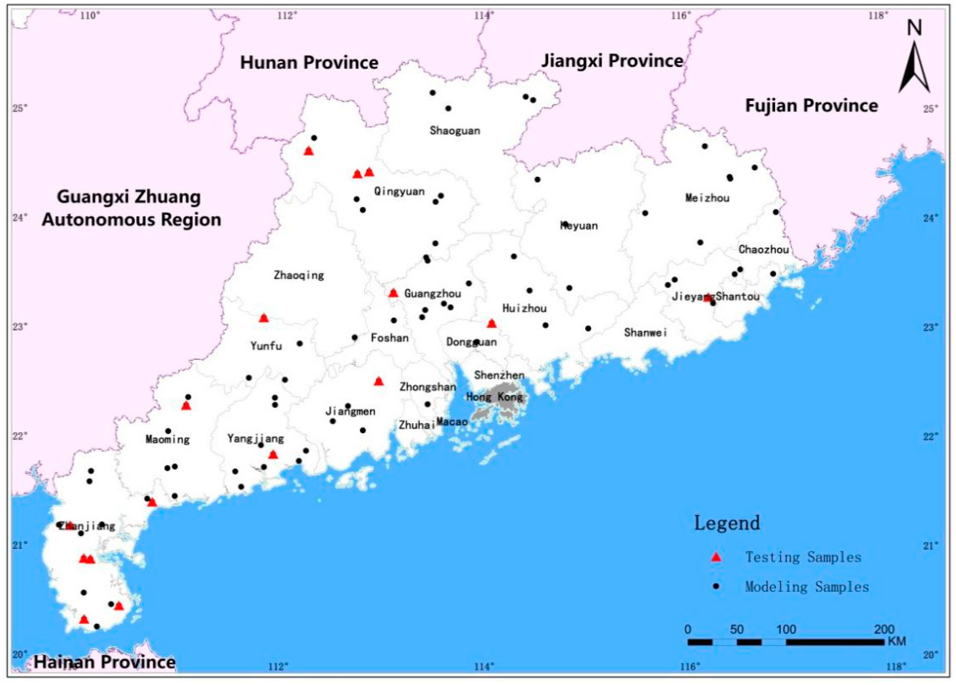
2.1. Study Site and Data

The study area is located in Guangdong Province of Southern China (Figure 1) and has a humid sub-tropical monsoon climate characterized by warm winters, hot summers, little frost or snow, sufficient precipitation, and sunshine. This study area has an annual average temperature of 19 °C–24 °C and a mean annual rainfall of 1300 mm–2500 mm. Guangdong has become a commercially developed area with abundant non-ferrous metals and rare metal resources. Heavy metal pollution in the soils has become a serious problem, due to the quick economic development. The contaminated soil reached 40% in the Pearl River Delta of Guangdong Province [14].
In this study, two datasets were collected from a total of 90 sample points. At each sample point, a soil sample of the top 0–20 cm depth was obtained to determine the contents of soil heavy metals: Cd, Hg and As, and hyperspectral reflectance data. The sample points were located using a global positioning system (GPS). The first dataset was composed of the data from 75 soil samples and collected during 22–24 June 2015, and out of which the data from 50 soil samples (black dots in Figure 1) were used to train the methods, and to establish the relationships between spectral variables and corresponding soil heavy metal contents. The data from the left 20 soil samples (red points in Figure 1) were used to assess the accuracy of the estimated soil heavy metal values. The second dataset consisted of the data collected from 15 sample points coinciding with the overpass time of HJ-1A satellite (30 October 2017) and was thus utilized to assess the feasibility of the developed model for the satellite data. The soil samples were air-dried at room temperature for three days to standardize the moisture level, and the small stones and plant residues were removed. The total of 90 soil samples were ground in an agate mortar. The ground soil samples were passed through a 20-mesh sieve (0.84 mm) in order to minimize the impact of particle size on soil spectral reflectance [15,16].

2.2. Experimental Data Pre-Processing

2.2.1. Chemical Analysis of Soil Properties

Prior to measuring the contents of the soil heavy metals, the soil samples were digested by hydrofluoric acid (HF)-nitric acid (HNO3)-perchloric acid (HCLO4) to determine the total contents of the three elements [17]. The digested soil samples were processed through an atomic fluorescence spectrometer to determine the Hg and As contents. The flame atomic absorption spectrometry (FAAS) was used to acquire the Cd content [4].

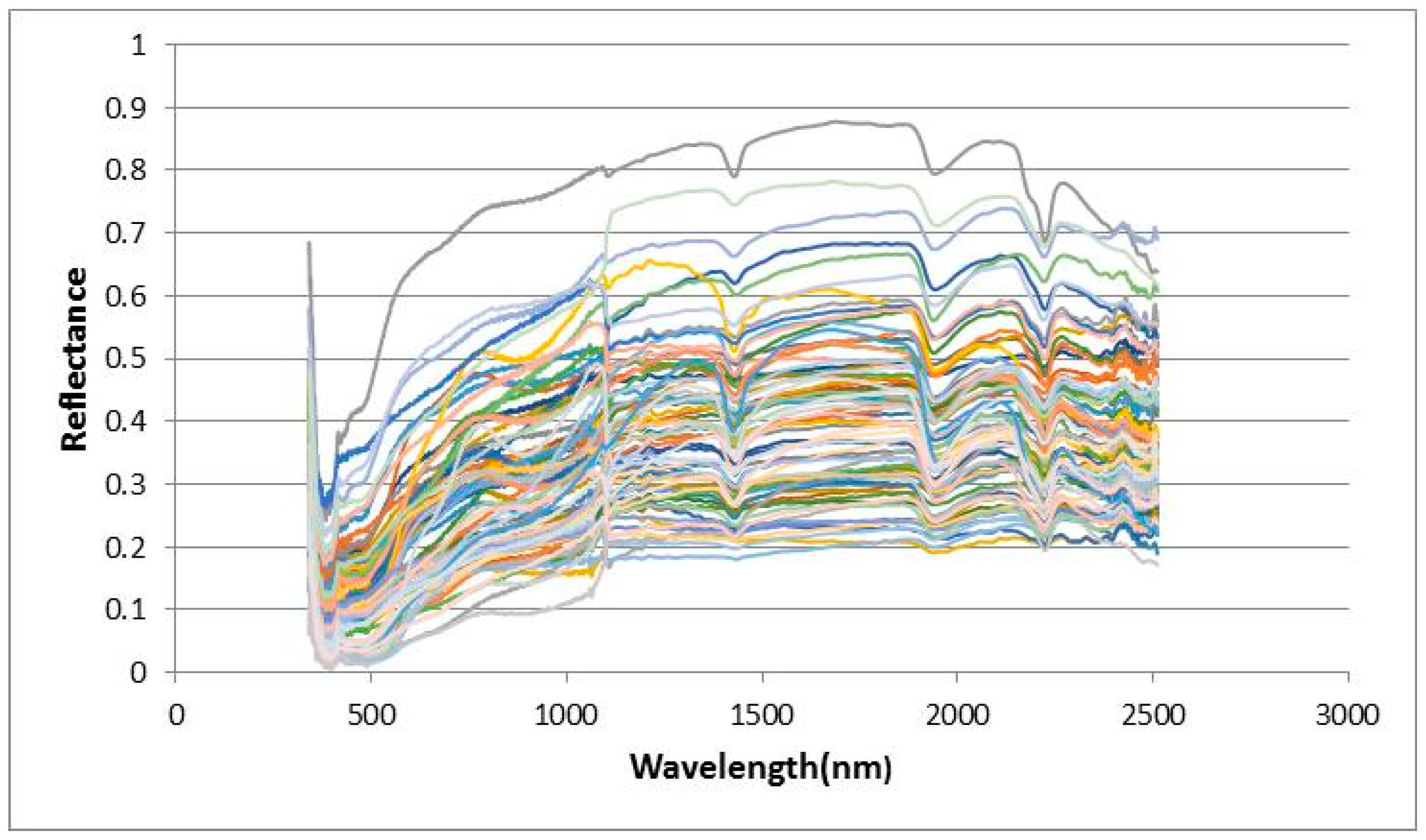
2.2.2. Spectral Measurements and Pre-Processing of Soil Samples

An AvaField portable spectrometer (Avantes, Inc., Holland) with a 340- 2511 nm spectrum was used to collect the spectral reflectance data of soil samples in a laboratory. The spectral sampling interval was 0.6 nm. The entire spectrometric experiment was performed in a black box. Each treated sample was placed in a black paper cup with a diameter of 10 cm and a depth greater than 5 cm. A 50W halogen lamp was used to estimate sunlight with a 10º field of view (FOV). The soil sample was subjected to soil reflection spectroscopy that is perpendicular to the soil sample. A white plate was used for calibration prior to collection in order to obtain the absolute reflectance. To mitigate the impact of instrument noise, the values of spectral bands (340.316 - 2511.179 nm) were initially smoothed using a Savitzky-Golay filter to obtain the stable spectrum curves. This method reduces the impact of glitch noise and purifies spectral information [18,19]. In order to obtain the spectral characteristics of the interest targets, the smoothed spectral data were transformed using the continuum removal (CR), the first derivative (FD), the second derivative (SD), the reciprocal transformation (RT), and the logarithm of reciprocal (LG), which could eliminate or reduce the effect of the background noise and the change in signal intensity caused by the soil surface spectral scattering and absorption. These transformation spectral data were used to build a mapping method with the soil heavy metals.

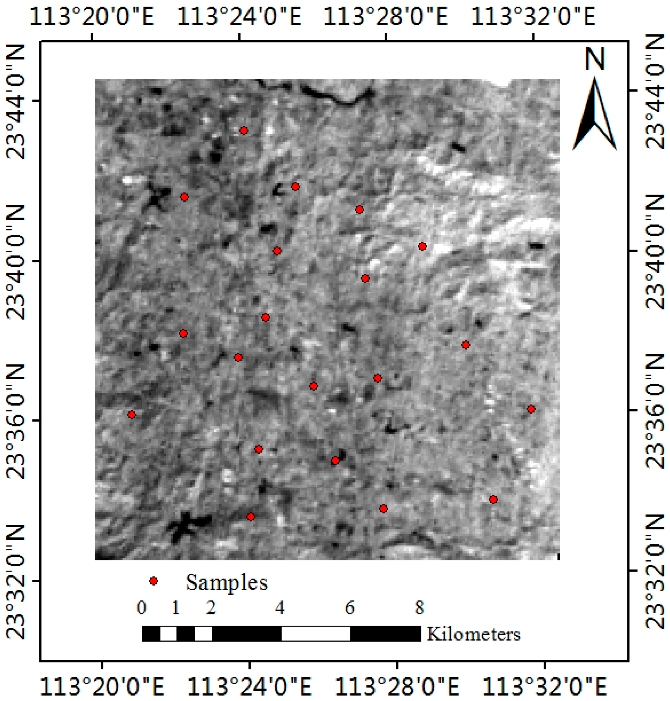
2.3. Image Acquisition and Preprocessing

In order to extend the application of the established model to hyperspectral satellite data, a HJ-1A satellite image (Path 457/Row 88, Scene PathBias A/ Scene RowBias 2) was acquired to retrieve the spatial distribution of soil heavy metal contents. The image was dated on 30 October 2017 and covered a part of Guangzhou, Guangdong province, China (23.53–23.77 °N and 113.2–113.48 °E) (Figure 2). It has a spatial resolution of 100 m, with a swath width of 50 km with a wavelength range of 459 nm–956 nm, a total of 115 bands, and a spectral interval of 5 nm. Although there was a narrower spectral range as compared with NASA’s widely used Earth Observing MODIS and EO-1 Hyperion, the HJ-1A HSI imaging spectrometer improved the spectral resolution for ground feature identification and information extraction [20].
To improve the relationships of spectral variables with the soil heavy metal contents in the study, the image enhancements, including stripe noise reduction, radiometric calibration, geometric rectification, and atmospheric correction were conducted. In this study, the moment matching method was applied to remove the stripe noise. The fast line-of-sight atmospheric analysis of spectral hyper-cubes (FLAASH) module in the environment for visualizing images (ENVI) system was used to perform atmospheric/radiometric correction for the HJ-1A satellite image. Geometric precision correction for HJ-1A HSI data was conducted using a quadratic polynomial model and the cubic convolution interpolation method, and the geometric correction errors were controlled within 0.5 pixels [21].

2.4. Selection of Optimum Spectral Variables

In this study, the Pearson product moment correlation was used to determinate the spectral variables that had the highest correlations with the contents of the soil heavy metals (Cd, Hg, and As). In order to eliminate the collinearity of the spectral variables, the variance inflation factor (VIF) was used [22] with the rules: 0 < VIF < 10, 10 ≤ VIF < 100 and VIF ≥ 100 indicating that no, strong, or severe multi-collinearity existed, respectively. According to the rules, the optimal spectral variables were selected and utilized as the input data of the network.

2.5. The BPNN Method to Estimate Soil Heavy Metal Contents

The BPNN is a parallel information processing method, able to work out complex, non-linear relationships by a learning model and by using experimental data [23]. The BPNN method has been widely used for prediction, data classification, characteristic recognition, and non-linear function approximation. The BPNN was used to estimate the heavy metal contents in the soil using a visible and near-infrared (VNIR) reflectance data. The topological structure of BPNN consisted of an input layer, a hidden layer, and an output layer. The input layer was composed of three or four nodes that represented the selected spectral variables that were used to estimate the response and the output layer consisted of one node, which represented the constituents of the heavy metals in the soils: Cd, As, and Hg. The number of nodes in the hidden layer was determined by a complex relationship between the transformed spectral variables and the soil heavy metal contents, which was a crucial parameter of BPNN. The BPNN is primarily divided into two processes during the training of experimental data: Forward propagation and error back propagation [24].
(1) Forward propagation: In neural networks, the neurons are linked between the current layer and the next one, but this connection is not within the same layer. Once a set of spectral variables were presented to the network, the input values were transmitted through the links to the hidden layer. Therefore, the equation of the output value was expressed as [24]:
H J = f ( i = 1 n w i j x i a i j )          j = 1 , 2 , , l
where H J indicates the output values in the jth hidden node, w i j represents the weights between the ith input node, and the jth hidden node, a j denotes the threshold value between the ith input node and jth hidden node, n is the number of spectral variables, and x i is the spectral value in band i.
The output value (H) in the hidden layer was transmitted to the output layer, and the equation of the output value was expressed as [24]:
O k = j = 1 l H j w j k b j k          k = 1 , 2 , , m  
where O k is the output values in the kth output node, w j k represents the weights between the jth hidden node, the kth output node, b j k denotes the threshold value between the jth hidden node and the kth output node, and l was the number of hidden nodes.
(2) Error back propagation: The output from the above forward propagation was compared with the real value to obtain an error. The error was propagated back to the network to improve the weights. This process was repeated until the error reached a specified threshold value. The equation of the error value was expressed as [24]:
e k = 1 2   j = 1 m ( Y k O k ) 2    k = 1 , 2 , , m
where e k represents the error between the output value in the kth output node and the real value of a soil heavy metal content, Y k is the real value of a soil heavy metal content, and O k is the output value in the kth output node.

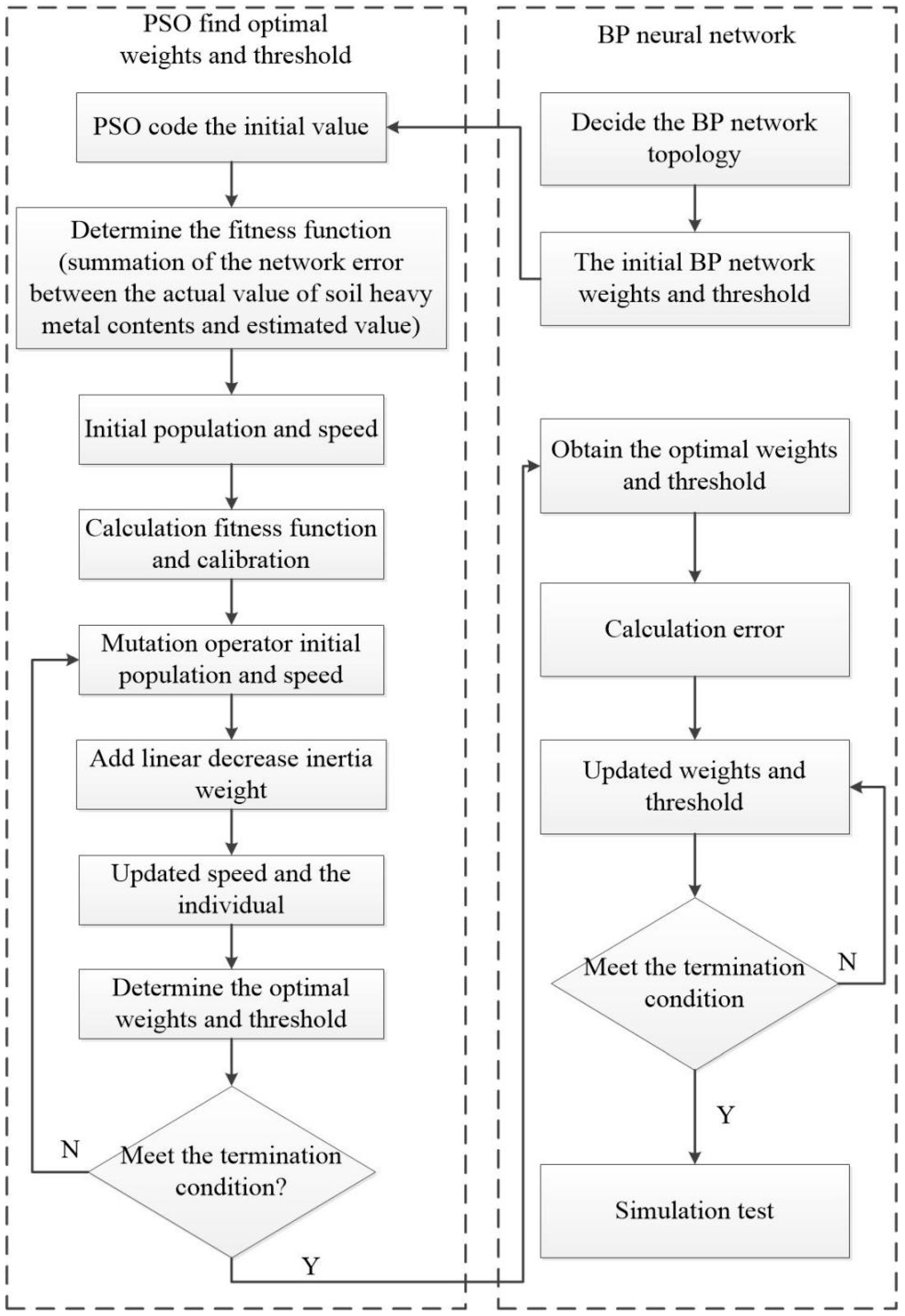
2.6. The PSO-BPNN Method to Estimate Soil Heavy Metal Contents

The particle swarm optimization (PSO) was initially introduced by Eberhart and Kennedy (1995) in order to solve the problems with continuous search space [25]. The PSO-BPNN combined the PSO algorithm’s global optimization ability and the BPNN algorithm’s local search advantage, which circumvented the slow convergence problem and avoided becoming trapped in a local minimum. The reaching process of BPNN is trained by the PSO algorithm, which has the position of each particle in the swarm that was represented as the weights and the thresholds of nodes in the BPNN. The network error between the actual value of a soil heavy metal content and the estimated value in the output layer was defined as the fitness function in the training. Each particle represented a candidate solution to minimize the network error. The optimum weights and thresholds were presented to determine the minimum network error. In the training experimental data process of PSO-BPNN, the spectral variables were selected as inputs of the networks and the outputs of networks were the heavy metal contents, including Hg, As, and Cd. The PSO algorithm that was used to train the BPNN’s weights and the threshold process is shown in Figure 3.

3. Results

3.1. Descriptive Statistics of Soil Properties in the Study Area

The statistics of the data for the heavy metals measured from the 75 soil samples is calculated in Table 1. The average values of Cd, Hg, and As contents were lower than the normative heavy metal contents, while their maximum values were much higher than the environment baseline values. The statistic results implied that the spatial distributions of three soil heavy metal contents were heterogenic in the study area.

3.2. Smoothing Spectral Data of Soil Heavy Metal Contents

When the spectral reflectance of the soil samples was measured, each soil sample was scanned at different positions three times, and five spectral curves were collected for each position in order to eliminate the instability of the measurements. The average value was obtained for each soil sample and smoothed using a Savitzky-Golay filter (Figure 4). The trend changes of the spectral reflectance curves of 75 soil samples were similar. Overall, the spectral reflectance values increased rapidly with the increased wavelength. The great changes occurred at the spectral interval (400 nm–600 nm), due to the spectral absorptions from the iron in the soil. The spectral reflectance values at the near-infrared spectral bands had small rates of changes but were higher than those in the visible spectral bands.

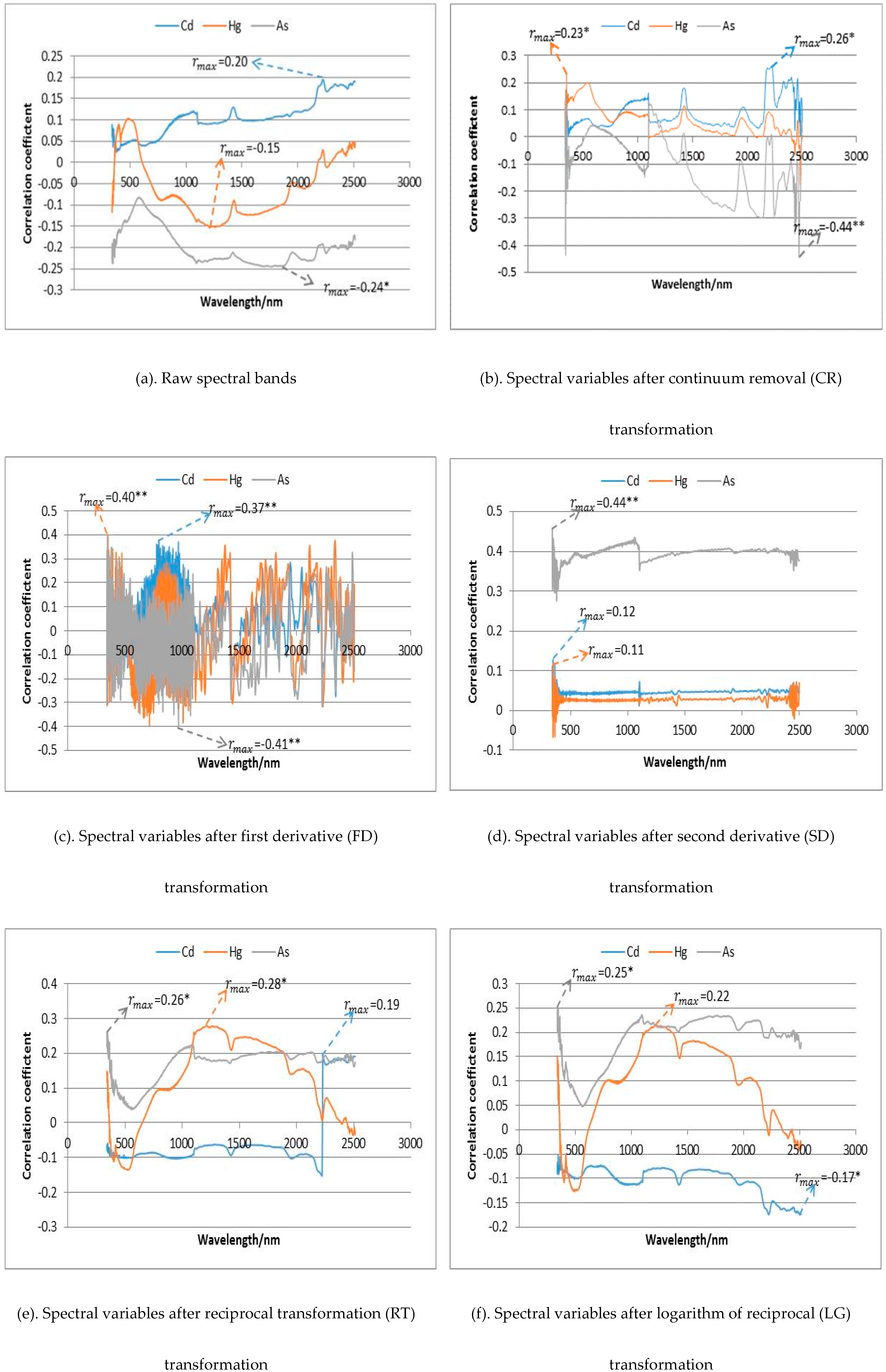
3.3. Optimal Spectral Variables for Retrieving Soil Heavy Metal Contents

The correlation coefficients between the soil heavy metal (Cd, Hg, and As) contents and the spectral variables, including raw spectral data and transformed spectral variables, are shown in Figure 5. The correlation analysis revealed that the spectral transformations further highlighted the relationships of the reflectance characteristics with the soil heavy metal contents, which are hidden in the soil spectra, when compared with the raw reflectance bands. The first derivative spectral data had higher correlations with the contents of the three soil heavy metals than the other spectral transformations. Nevertheless, it was difficult to accurately model the relationships of the spectral characteristic with the soil heavy metal contents when the correlation coefficients were smaller than 0.4.
In order to improve the estimation accuracies of the soil heavy metal contents, we further used the spectral variables with the maximum correlation coefficients to develop new spectral variables. That is, the combinations of spectral variables by the calculations of addition, subtraction, multiplication, and division operations. Table 2 shows the combined spectral variables that had the highest correlations with the soil heavy metal (Cd, Hg, and As) contents, which suggested that the combined spectral variables greatly improved the correlations with a range of the coefficients from 0.36 to 0.60, being significant at the significant level of 0.01.
To eliminate the multicollinearity among the combined spectral variables, the VIF analysis was performed in Table 3. The combined spectral variables were selected according to the following criteria: The greatest value of adjusted coefficient (R2) of determination; the statistically significant P-value of the partial F-test; and the VIF value of less than 10. The selected combinations of the spectral variables reduced the duplication of information and provided the potential of effectively accounting for the spatial variability of the soil heavy metal contents. They were considered to be optimal.

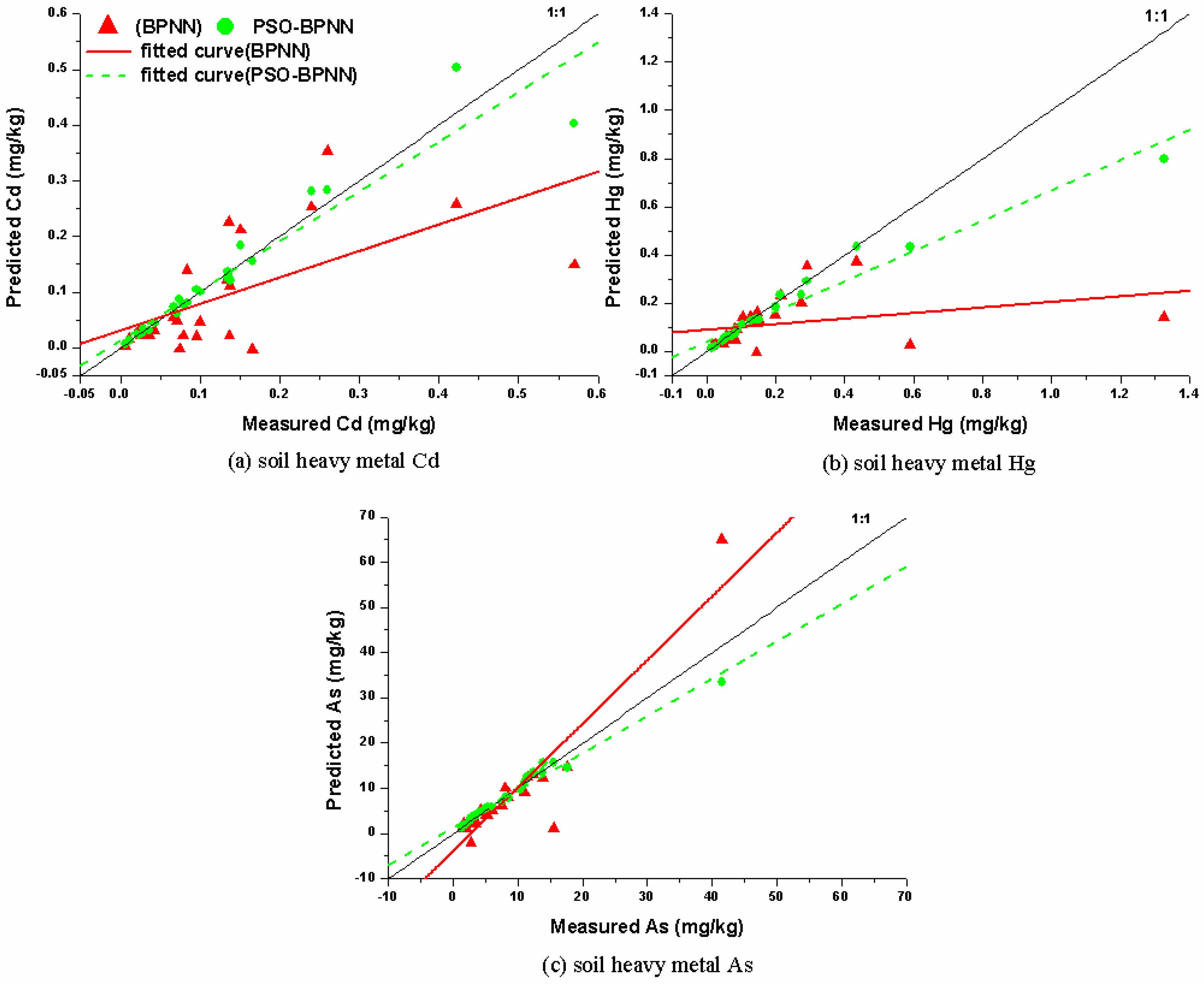
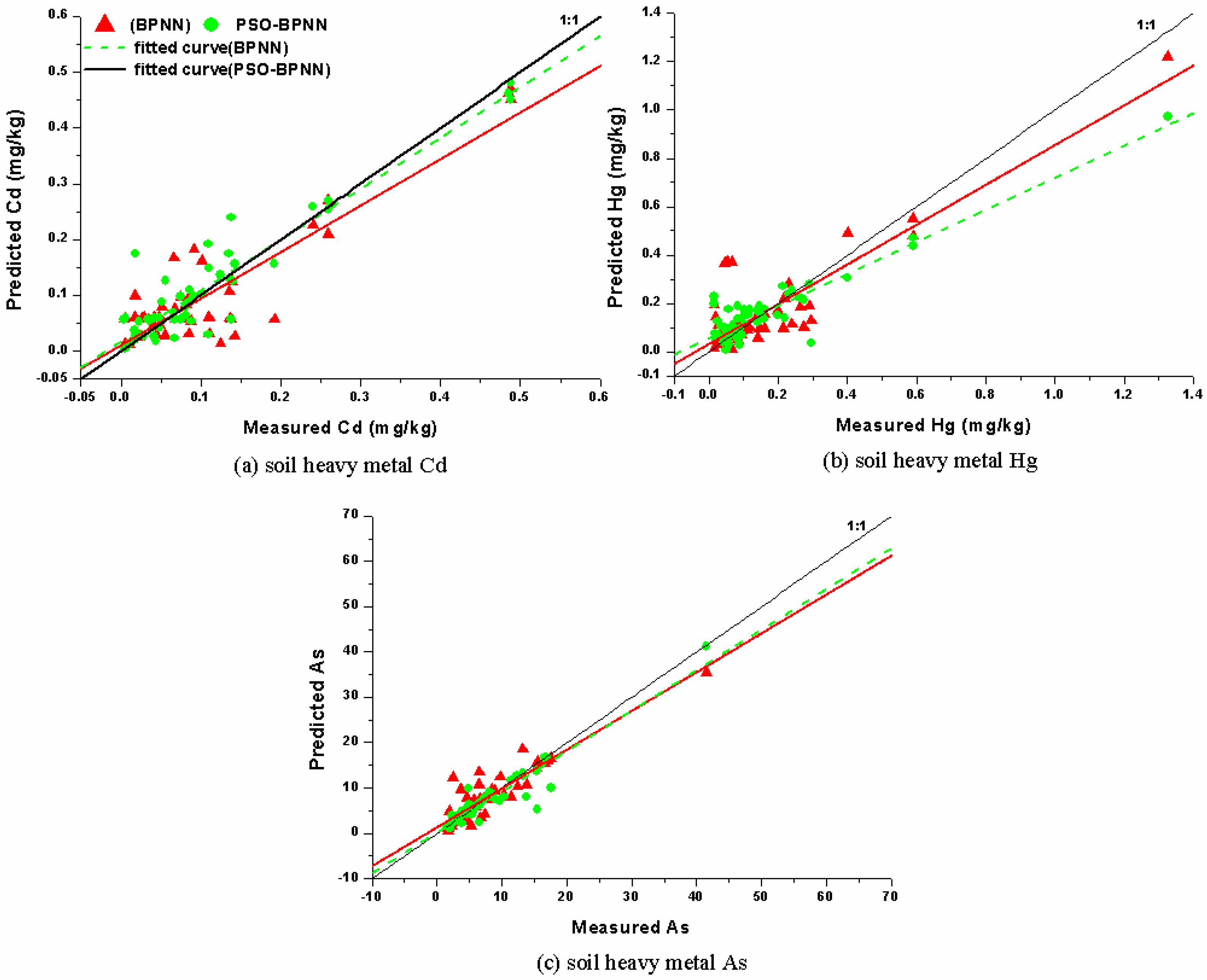
3.4. Estimation and Accuracy Validation of Soil Heavy Metal Contents for Soil Sample Points

Both BPNN and PSO-BPNN method were used and compared to estimate the contents of the soil heavy metal: Cd, Hg, and As. For both methods, the input layer in the neural network was composed of two nodes for Cd and three nodes for Hg and As. The output layer consisted of the soil heavy metal contents. The two nodes were used in the hidden layer to train the networks. For both BPNN and PSO-BPNN, 50 training samples were randomly selected to train the response relationships between the soil heavy metal contents and the optimal spectral variables (Figure 6). For both Cd and Hg, obviously, BPNN led to over-estimations for the smaller values and under-estimations for the larger values, and the PSO-BPNN greatly mitigated the over-estimations and underestimations. For As, BPNN resulted in under-estimations for some of the smaller values and overestimation for the largest value, and the PSO-BPNN created reverse results with smaller biases. This implied that overall, PSO-BPNN improved the modeling of the soil heavy metal contents.
In order to validate the estimation accuracy of both methods for the soil heavy metal contents, 25 test samples were used to create the predictions of the soil heavy metal contents (Figure 7). Most of the scattered points for the estimated contents of all the soil heavy metals versus the measured values were distributed around the 1:1 line. For Cd and Hg, however, BPNN led to over-estimations for the smaller values and under-estimations for the larger values. The PSO-BPNN reduced the over-estimations and under-estimations of Cd content. For Hg, although the under-estimation by PSO-BPNN for the largest value was more obvious than by BPNN, overall the estimates from PSO-BPNN were closer to the line of 1:1 than those from BPNN. Moreover, the predicted contents of As from BPNN and PSO-BPNN had a similar trend, but the scatter points of the predictions from PSO-BPNN were closer to the line of 1:1 than those from BPNN.
The predicted contents of the soil heavy metals, from BPNN and PSO-BPNN, were further compared with the field observations from 25 test samples by calculating the coefficient of determination (R2), the mean relative error (MRE), and the relative RMSE (RRMSE) in Table 4. The estimates from PSO-BPNN were more accurate than those from BPNN. Compared with BPNN, PSO-BPNN decreased the MRE by 68% to 71% and the RRMSE by 64% to 67%. For all three soil heavy metal contents, PSO-BPNN also significantly increased the coefficients of determination. The improvements were thus statistically very significant.

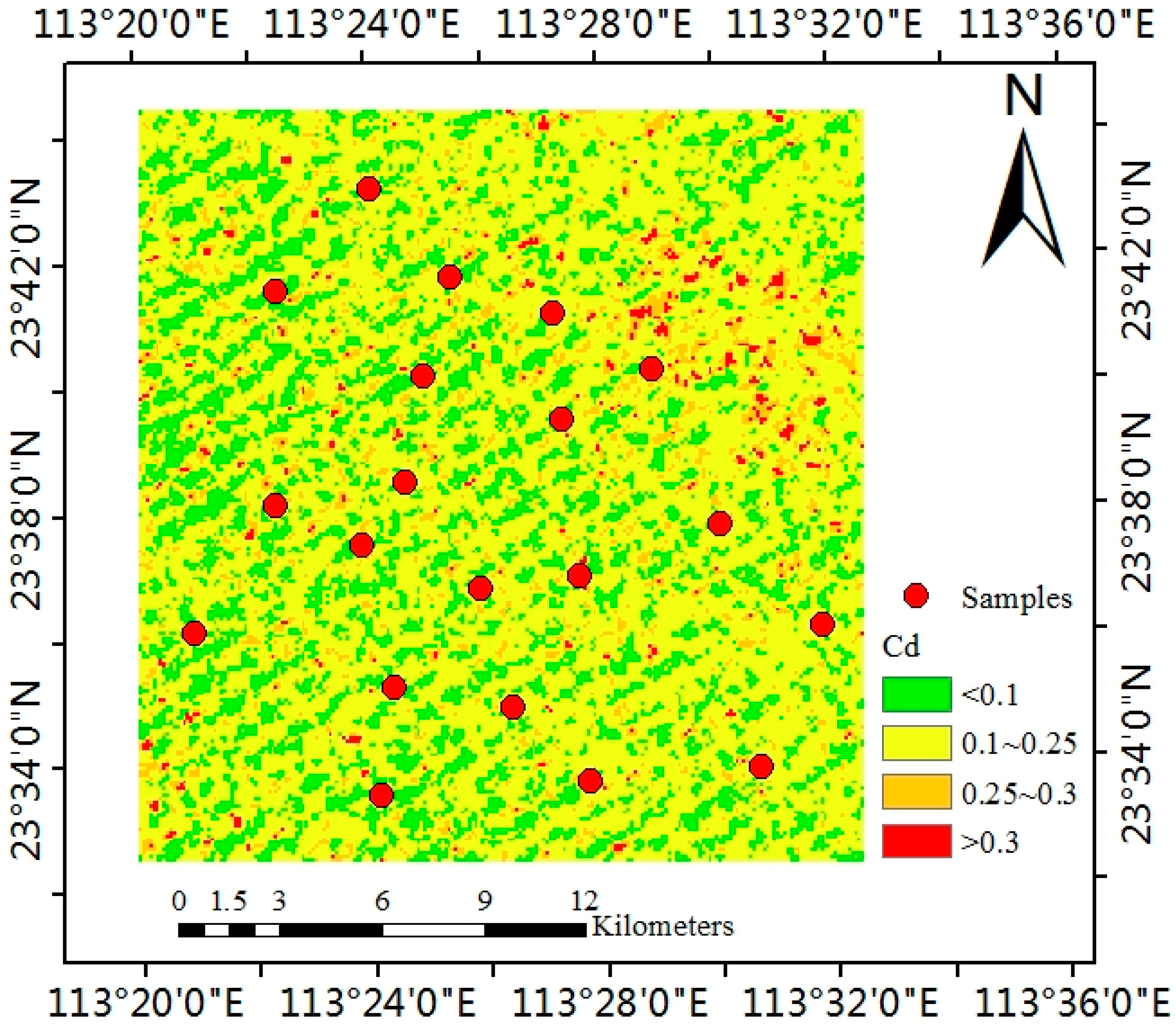
3.5. Estimation and Accuracy Validation of Soil Heavy Metal Contents at the Regional Scale

In this study, only the PSO-BPNN method was used to map the spatial patterns of soil heavy metal Cd content. To obtain consistent bands of HJ-1A HSI image, the filed measured spectral data were spectrally re-sampled by stepwise merging adjacent bands. The re-sampled bands were then selected to yield the optimal spectral variables. Finally, four bands, including B114: 942.705 nm, B94: 795.065 nm, B16: 493.590 nm and B92: 782.805 nm, were selected to construct the HSI-based PSO-BPNN model to map the content of soil heavy metal Cd (Figure 8).
In order to validate the feasibility of PSO-BPNN to estimate the content of soil heavy metal Cd at the regional scale, the values of the field measured Cd content were compared with its estimates (Table 5). The HSI-based PSO-BPNN model explained 65.6% of the variance in Cd content with an RRMSE of 35.989%. The mean value of the measured contents of Cd was close to the average value of the estimates. Their difference was no significantly different from zero, indicating that PSO-BPNN was capable of estimating Cd content at the regional scale.

4. Discussion

Soil heavy metals, such as Cd, Hg, and As contaminate soils and thus endanger human life and deteriorate the environment. Accurately estimating and mapping the contents of the soil heavy metals and monitoring their dynamics become critical. Hyper-spectral data provide the potential data for monitoring scale-regional soil heavy metal contents, by developing and using the relationship of hyperspectral bands and various transformations with the soil heavy metals. However, the availability of a large number of hyperspectral bands leads to the difficulty of selecting the spectral variables that have significant contributions in improving the estimation of soil heavy metal contents [3,4,5]. Traditionally, a correlation analysis of hyperspectral data with soil heavy metal contents has been widely used [26,27]. But, the correlation analysis ignores collinearity and duplication of information among the hyperspectral bands, which often results in low estimation accuracy. In this study, we integrated the correlation analysis and VIF analysis for the selection of the hyperspectral data collected in the field, their transformations (FD, SD, LG, RT, etc.), and the combinations of the transformations by addition, subtraction, multiplication, and division. This process did not only lead to the spectral variables that had highest correlations with the contents of the soil heavy metals, but also eliminated the spectral variables that were highly correlated with each other and had information duplication. It was found that compared with the original hyperspectral bands and their transformations, the combined spectral variables greatly improved the correlations with the contents of the soil heavy metals. This indicated that the relationships of the soil heavy metal contents with the spectral variables are complicated and could not be well-explained by the simple hyperspectral bands and their transformations. This finding was supported by the studies of Kemper and Sommer (2002) [8] and Wu et al. (2005) [19].
Another big challenge of using hyperspectral data to map the contents of the soil heavy metals for a large area was the development of spatial interpolation algorithms that can be used to account for the relationships of the selected spectral variables with the contents of the soil heavy metals [6,7,8,9,10]. Previous studies [11,12,28] demonstrated that the BPNN method was a good alternative. However, the large uncertainties of the input initial parameters affected the improvement of estimation accuracy for the contents of the soil heavy metals [29]. In this study, the PSO algorithm was introduced to BPNN, which led to an integrated PSO-BPNN method to optimize the initial parameter values. The research results showed that the PSO-BPNN method significantly increased the estimation accuracies of the soil heavy metal contents by greatly decreasing the MRE and RRMSE values. The superiority of PSO-BPNN was attributed to the optimization of the initial input parameters (thresholds and weights) for BPNN by the PSO algorithm, which resulted in the solution for the problem of being stuck in the local minima [8,30]. This implies that PSO-BPNN is very promising in improving the estimation and mapping of the soil heavy metal contents using hyperspectral imagery.
In order to validate the regional-scale applicability of PSO-BPNN, the HJ-1A data were used to map the soil heavy metal Cd content. The results of validation using the test sample data showed that the selected spectral variables explained 65.6% of the variance in Cd content and led to an RRMSE of 36% for mapping Cd content. This indicated that PSO-BPNN had great potential to map the soil heavy metal Cd content at a large scale. However, compared with that using the hyperspectral data collected in the field, the estimation accuracy of the soil heavy metal Cd using the HJ-1A image was lower. The reason might be mainly due to the effect of vegetation canopies in the HJ-1A image and its coarser spectral resolution [31]. Thus, in order to eliminate the vegetation canopy effect, the extraction and consideration of soil component using a spectral unmixing technique should be a focus of future research.
On the other hand, most of the soil sample data, used to train BPNN and PSO-BPNN, had low contents of the soil heavy metals. This led to larger errors for the test samples that had high heavy metal contents and affected performance and prediction accuracy [32]. Thus, in order to improve the prediction accuracy of the soil heavy metal contents, more soil samples with high values of the contents have to be collected to improve the performance of PSO-BPNN in the future.
Finally, in this study only the soil heavy metal Cd content was mapped by PSO-BPNN, due to the limitation of the HJ-1A HSI data with 450 nm–960 nm. Future research that would map the contents of Hg and As, using satellite hyperspectral images, may be followed through the Chinese hyperspectral satellite Gaofen-5 data, which covers a wider spectral region of 400 nm–2500 nm.

5. Conclusions

In this study, the integrated PSO-BPNN method was developed and used to improve the estimation accuracy of the soil heavy metal (Cd, Hg, and As) contents in the soil samples collected in Guangdong, which is one of the most developed provinces in China. The following conclusions could be drawn: (1) Based on the sample averages, overall the contents of the soil heavy metals did not exceed the normative heavy metal contents, but the sample maximum values were higher than the corresponding environment baseline values; (2) the combined spectral variables had a stronger capacity of explaining variances of the soil heavy metals than the original spectral data and transformed spectral variables; (3) compared with BPNN, PSO-BPNN significantly increased the estimation accuracy of the soil heavy metal contents by decreasing the MRE and RRMSE by 68% to 71% and 64% to 67%, respectively; and (4) PSO-BPNN, coupled with a HJ-1A hyperspectral image also led to an acceptable accuracy of mapping the Cd content at a regional scale. This indicated that PSO-BPNN provided great potential to accurately estimate the soil heavy metal contents.

Author Contributions

Z.L. and P.L. conceived and designed the experiments; P.L. analyzed the data, created the tables and figures, and finished the first version of the paper; Z.L., Y.H., Z.S., Y.P. and L.W. contributed valuable opinions during the manuscript writing; G.W. revised the whole manuscript. All authors read and approved the final manuscript.

Funding

This research was supported by the National Key Research and Development Program of China (“Source Identification and Contamination Characteristics of Heavy Metals in Agricultural Land and Products”, 2016YFD0800301), the Guangdong Provincial Science and Technology Project of China (2017A050501031), and the Guangzhou Science and Technology Project, China (201804020034).

Conflicts of Interest

The authors declare no conflict of interest.

References

  1. Mouazen, A.; Maleki, M.; De Baerdemaeker, J.; Ramon, H. On-line measurement of some selected soil properties using a VIS-NIR sensor. Soil Tillage Res. 2007, 93, 13–27. [Google Scholar] [CrossRef]
  2. Jarmer, T.; Vohland, M.; Lilienthal, H.; Schnug, E. Estimation of some chemical properties of an agricultural soil by spectroradiometric measurements. Pedosphere 2008, 18, 163–170. [Google Scholar] [CrossRef]
  3. Tan, K.; Ye, Y.; Cao, Q.; Du, P.; Dong, J. Estimation of arsenic contamination in reclaimed agricultural soils using reflectance spectroscopy and ANFIS method. IEEE J.-STARS 2014, 7, 2540–2546. [Google Scholar]
  4. Wu, D.W.; Wu, Y.Z.; Ma, H.R. Study on the prediction of soil heavy metal elements content based on Mid-Infrared diffuse reflectance spectra. Spectrosc. Spectr. Anal. 2009, 29, 114. [Google Scholar]
  5. Kooistra, L.; Wanders, J.; Epema, G.; Leuven, R.; Wehrens, R.; Buydens, L. The potential of field spectroscopy for the assessment of sediment properties in river floodplains. Anal. Chim. Acta 2003, 484, 189–200. [Google Scholar] [CrossRef]
  6. Lian, S.; Jian, J.; Tan, D.J.; Xie, H.B.; Luo, Z.F.; Gao, B. Estimate of heavy metals in soil and streams using combined geochemistry and field spectroscopy in Wansheng mining area, Chongqing, China. Int. J. Appl. Earth. Obs. 2015, 34, 1–9. [Google Scholar]
  7. Lu, P.; Wang, L.; Niu, Z.; Li, L.; Zhang, W. Prediction of soil properties using laboratory VIS-NIR spectroscopy and Hyperion imagery. J. Geochem. Explor. 2013, 132, 26–33. [Google Scholar] [CrossRef]
  8. Kemper, T.; Sommer, S. Estimate of heavy metal contamination in soil after a mining accident using reflectance spectroscopy. Environ. Sci. Technol. 2002, 36, 2742–2747. [Google Scholar] [CrossRef] [PubMed]
  9. He, J.L.; Jiang, J.J.; Zhou, S.L.; Xu, J.; Cai, H.L.; Zhang, C.Y. The hyperspectral characteristics and retrieval of soil organic matter content. Sci. Agric. Sin. 2007, 40, 638–643. [Google Scholar]
  10. Zhang, Q.X.; Zhang, H.B.; Liu, W.K.; Zhao, S.X. Inversion of heavy metals content with hyperspectral reflectance in soil of well-facilitied capital farmland construction areas. Trans. Chin. Soc. Agric. Eng. 2017, 33, 230–239. [Google Scholar]
  11. Ghadimi, F. Prediction of heavy metals contamination in the groundwater of Arak region using artificial neural network and multiple linear regression. J. Tethys. 2015, 3, 203–215. [Google Scholar]
  12. Gandhimathi, A.; Meenambal, T. Spatial prediction of heavy metal pollution for soils in Coimbatore, India based on ANN and kriging method. Eur. Sci. J. 2012, 8, 1857. [Google Scholar]
  13. Guo, Y.K.; Liu, L.; Liu, N.; Zhu, S.T.; Li, D. The prediction of the heavy metal Fe content in rice field based on support vector machine regression. Beijing Surv. Map. 2017, 6, 10–13. [Google Scholar]
  14. Guo, Z.X.; Wang, J.; Chai, M.; Chen, Z.P.; Zhan, Z.S.; Zheng, W.P.; Wei, X.G. Spatiotemporal variation of soil pH in Guangdong Province of China in past 30 years. Chin. J. Appl. Ecol. 2011, 22, 425–430. [Google Scholar]
  15. Chang, C.W.; Laird, D.A.; Mausbach, M.J.; Hurburgh, C.R., Jr. Near-infrared reflectance spectroscopy-principal components regression analyses of soil properties. Soil Sci. Soc. Am. J. 2001, 65, 480–490. [Google Scholar] [CrossRef]
  16. Kooistra, L.; Wehrens, R.; Leuven, R.; Buydens, L. Possibilities of visible-near-infrared spectroscopy for the assessment of soil contamination in river floodplains. Anal. Chim. Acta 2001, 446, 97–105. [Google Scholar] [CrossRef]
  17. Wang, J.J.; Cui, L.J.; Gao, W.X.; Shi, T.Z.; Chen, Y.; Gao, Y. Prediction of low heavy metal concentrations in agricultural soils using visible and near-infrared reflectance spectroscopy. Geoderma 2014, 216, 1–9. [Google Scholar] [CrossRef]
  18. Gomez, C.; Lagacherie, P.; Coulouma, G. Continuum removal versus PLSR method for clay and calcium carbonate content estimation from laboratory and airborne hyperspectral measurements. Geoderma 2008, 148, 141–148. [Google Scholar] [CrossRef]
  19. Wu, Y.; Chen, J.; Wu, X.; Tian, Q.; Ji, J.; Qin, Z. Possibilities of reflectance spectroscopy for the assessment of contaminant elements in suburban soils. Appl. Geochem. 2005, 20, 1051–1059. [Google Scholar] [CrossRef]
  20. Tian, H.J.; Cao, C.X.; Xu, M.; Zhu, Z.C.; Liu, D.; Liu, D.; Wang, X.Q.; Cui, S.H. Estimation of chlorophyll-a concentration in coastal waters with HJ-1A HSI data using a three-band bio-optical model and validation. Int. J. Remote Sens. 2014, 35, 5984–6003. [Google Scholar] [CrossRef]
  21. Anne, N.J.P.; Abd-Elrahman, A.H.; Lewis, D.B.; Hewitt, N.A. Modeling soil parameters using hyperspectral image reflectance in subtropical coastal wetlands. Int. J. Appl. Earth Obs. Geoinform. 2014, 33, 47–56. [Google Scholar] [CrossRef]
  22. Gómez, R.S.; Pérez, J.G.; Martín, M.D.L.; García, C.G. Collinearity diagnostic applied in ridge estimation through the variance inflation factor. J. Appl. Stat. 2016, 43, 19. [Google Scholar]
  23. Wu, J.H.; Wang, G.L.; Wang, J.; Su, Y. BP neural network and multiple linear regression in acute hospitalization costs in the comparative study. J. Fluid Mech. 2011, 5, 50–51. [Google Scholar] [CrossRef]
  24. Yu, X.; Efe, M.O.; Kaynak, O. A general backpropagation algorithm for feedforward neural network learning. IEEE Trans. Neural Netw. 2002, 13, 251–254. [Google Scholar] [PubMed]
  25. Kennedy, J.; Eberhart, R. Particle Swarm Optimization. In Proceedings of the Fourth IEEE International Conference on Neural Networks, Perth, Australia, 27 November–1 December 1995; Volume 4, pp. 1942–1948. [Google Scholar]
  26. Singh, A.N. Estimation of as and cu contamination in agricultural soils around a mining area by reflectance spectroscopy: A case study. Pedosphere 2009, 9, 719–726. [Google Scholar]
  27. Liu, M.; Liu, X.; Li, M.; Fang, M.; Chi, W. Neural-network model for estimating leaf chlorophyll concentration in rice under stress from heavy metals using four spectral indices. Biosyst. Eng. 2010, 106, 223–233. [Google Scholar] [CrossRef]
  28. Pandit, C.; Filippelli, G.; Lin, L. Estimation of heavy-metal contamination in soil using reflectance spectroscopy and partial least-squares regression. Int. J. Remote Sens. 2010, 31, 13. [Google Scholar] [CrossRef]
  29. Wang, F.; Gao, J.; Zha, Y. Hyperspectral sensing of heavy metals in soil and vegetation: Feasibility and challenges. ISPRS J. Photogramm. Remote Sens. 2018, 136, 73–84. [Google Scholar] [CrossRef]
  30. Khosravi, V.; Ardejani, F.D.; Yousefi, S.; Aryafar, A. Monitoring soil lead and zinc contents via combination of spectroscopy with extreme learning machine and other data mining methods. Geofis. Int. 2018, 318, 29–41. [Google Scholar] [CrossRef]
  31. Luo, H.; Zheng, Y. The comparison of citrus canopy spectral characteristics obtained by the HJ-1A/ HSI and ASD field spectrometer. In Proceedings of the 9th IEEE International Conference on Fuzzy Systems and Knowledge Discovery, Sichuan, China, 29–31 May 2012; pp. 650–655. [Google Scholar]
  32. Sadr, M.H.; Astaraki, S.; Salehi, S. Improving the neural network method for finite element model updating using homogenous distribution of design points. Arch. Appl. Mech. 2007, 77, 795–807. [Google Scholar] [CrossRef]
Figure 1. The study area and the distribution of soil sample points (black dots and red triangles represented training and test samples, respectively).
Sustainability 11 00419 g001
Figure 2. The area covered by the HJ-1A image and the locations of the soil samples (red dots).
Sustainability 11 00419 g002
Figure 3. The flow chart of the particle swarm optimization (PSO) algorithm used to optimize the back propagation neural network (BPNN) weights and the threshold.
Sustainability 11 00419 g003
Figure 4. The curves of the soil spectral reflectance values.
Sustainability 11 00419 g004
Figure 5. The correlation coefficients between the Cd, Hg, and As concentrations and the various spectral variables: (a) Raw spectral bands; (b) Spectral variables after CR transformation; (c) Spectral variables after FD transformation; (d) Spectral variables after SD transformation; (e) Spectral variables after RT transformation; and (f) Spectral variables after LG transformation (rmax is the highest correlation coefficient between the soil heavy metal contents and the spectral variables; * and ** mean that correlation was significant at the 0.05 and 0.01 level, respectively).
Sustainability 11 00419 g005
Figure 6. The scatter plots of the predicted versus measured heavy metal contents (Cd, Hg, and As) using the training dataset and both BPNN and PSO-BPNN method. (a) Soil heavy metal Cd; (b) Soil heavy metal Hg; (c) Soil heavy metal As.
Sustainability 11 00419 g006
Figure 7. The scatter plots of the predicted values against the measured contents of Cd, Hg, and As. (a) Soil heavy metal Cd; (b) Soil heavy metal Hg; (c) Soil heavy metal As.
Sustainability 11 00419 g007
Figure 8. The spatial distribution of soil heavy metal Cd content and sampling points.
Sustainability 11 00419 g008
Table 1. Statistical values for the measured contents of soil heavy metals of the study area.
Metal (mg/kg)MinimumMaximumMeanSDCV (%)Background ValueStandard
Cd0.0030.5700.1740.11163.790.0340.3
Hg0.0260.3100.1320.08564.440.0780.3
As1.37068.6009.7617.48776.7010.5030
Table 2. The greatest correlation coefficients between the soil heavy metal contents and the combined spectral variables (* and ** mean that the correlation was significant at the 0.05 and 0.1 level, respectively).
Heavy MetalSpectral ParametersCombinations of Spectral Variablesr
CdRaw Reflectance (R)R1089.379 *R2222.4240.36 **
First Derivative (FD)FD938.753 *FD795.2310.60 **
Second Derivative (SD)SD346.839 *SD808.196−0.54 **
Logarithm of Reciprocal (LG)LG784.504/LG492.4420.42 **
Reciprocal Transformation (RT)RT2253.954/RT2228.7330.40 **
Continuum Removal (CR)CR348.024 − CR2222.424−0.48 **
HgRaw Reflectance (R)R2222.424/R1219.6770.38 **
First Derivative (FD)FD1373.48 + 7 *FD430.210.58 **
Second Derivative (SD)30 *SD356.912 − 25 *SD348.024−0.43 **
Logarithm of Reciprocal (LG)LG2222.424 − LG1212.22−0.47 **
Reciprocal Transformation (RT)7 *RT2222.424–12 *RT1212.22−0.42 **
Continuum Removal (CR)CR2486.193 − CR350.987−0.48 **
AsRaw Reflectance (R)R347.431 + R1765.023−0.36 **
First Derivative (FD)FD2342.058/FD966.869−0.60 **
Second Derivative (SD)6 *SD363.425–5 *SD340.316−0.49 **
Logarithm of Reciprocal (LG)LG345.653 − LG344.467−0.40 **
Reciprocal Transformation (RT)RT343.291/RT343.874−0.49 **
Continuum Removal (CR)CR344.467 − CR2473.69−0.54 **
Table 3. The combined spectral variables selected and corresponding criteria.
Heavy MetalCombined Spectral VariablesAdjusted R2Estimation ErrorFSignificance LevelVariance Inflation Factor
CdFD938.753*FD795.231, LG784.504/LG492.4420.2260.34315.4130.0004.045
HgFD1373.48 + 7*FD430.21, LG2222.424 − LG1212.22, 7*RT2222.424 − 12*RT1212.220.3000.2357.7810.0006.324
AsFD2342.058/FD966.869, RT343.281/RT343.874, 6*SD363.425 − 5*SD340.3160.3127.87415.4270.0005.006
Table 4. The estimation accuracies of soil heavy metal contents using BPNN and PSO-BPNN methods based on the test dataset.
BPNNPSO-BPNN
Heavy MetalR2Mean Relative Error (MRE)
(%)
RRMSE
(%)
R2MRE
(%)
RRMSE
(%)
Cd0.39034.05336.2170.75510.07412.037
Hg0.28337.78438.5140.74210.90913.862
As0.51629.95530.9700.8119.59411.121
Table 5. Comparison between the measured and estimated values for soil heavy metal Cd content (mg·kg−1).
CategoryMaximum MinimumMeanStandard DeviationR2RRMSE (%)
Measured value 0.2180.0680.1370.0440.65635.989
Estimated value0.2490.0320.1220.053

