Understanding Urban Mobility Pattern with Cellular Phone Data: A Case Study of Residents and Travelers in Nanjing

Abstract

The rapid development of urban metropolises has attracted a growing number of immigrants and travelers, increasing the burden on transportation systems. Previous research on urban mobility patterns have ignored the temporal variations and heterogeneity in divergent urban trip makers due to the limited data resolution and coverage. In this paper, we analyzed cellular phone data of more than five million travelers for one month in Nanjing, China and proposed a method to extract trip origin and destination information from cellular phone signal data. We found that mobility patterns are different for urban residents, short-term travelers, and transfer travelers, and that trip length distributions can best be described by gamma and exponential distributions. In addition to the daily trip length distribution models, we utilized the agglomerative hieratical clustering method in order to group similar hourly trip patterns and further proposed within-day trip length distribution models under different times of the day and days of the week.

1. Introduction

Understanding urban mobility patterns is essential in transportation engineering, such as the estimation of trip distributions in the transportation planning procedures, and traffic forecasting in traffic management. Traditional urban mobility information acquisition relies on urban residents’ travel surveys. In traditional travel surveys, methods such as questionnaires and telephone inquiries are used to obtain travel information such as travel destinations, travel time, and travel modes. The process takes a lot of manpower and the cost is expensive. Moreover, the accuracy of the self-reported travel times and distances has raised serious questions. The participants of the surveys are mostly residents of the city and travelers are often neglected from those kinds of surveys. However, these travelers contribute a huge number of trips, especially in large metropolitan areas.

With the rapid development of telecommunication technology, new pervasive data collection methods such as GPS and cellular phone technology have appeared to provide auxiliary traffic information sources with a larger sample size at a lower cost. Although GPS techniques could provide more accurate positioning results for individual users, vendors such as navigation providers have difficulty collecting a sufficiently large sample size compared with cellular phone service providers. Users may not use a navigation service for every trip, especially for their routine commuting trips, however cellular phone services can passively collect people’s trajectories as long as the users turn their phone on. With cellular phone data, we can extract the trip information from a large population size, including both residents and travelers. Currently, the difficulty of utilizing cellular phone data lies in its huge volume, and more efficient procedures are needed for extracting useful information from these large data sets.

This paper contributes to this effort by identifying different mobility patterns in a heterogeneous population group, including residents, short-term travelers, and transfer travelers using cellular phone data. The methodology developed for identifying trip ends using cellular phone data is proposed, followed by the results of a statistical analysis to model trip-length distributions for heterogeneous travelers at various time periods. These results might be useful for estimating origin–destination information for transportation planners.

2. Related Work

The trip pattern of human mobility is extremely important in a variety of applications, including crowd flow forecasting [1,2], public transportation planning [3], and urban planning [4] among others, which constitutes the basis of urban transportation planning management technology.

In urban transportation planning studies, the estimation of future travel demand involves four steps: trip generation modelling, trip distribution modelling, modal split, and trip assignment. The trip distribution model estimates the number of trips made between each traffic analysis zone using the result from the previous trip generation modelling step, which relies on spatial interaction models, such as gravity and intervening opportunity models. Trip length distribution is an essential part of the trip distribution modelling step and describes the pattern in which travel demand decreases with a certain impedance variable (distance, travel time, or generalized cost). The improvement in the accuracy of the trip length distribution model is beneficial to the subsequent transportation modelling tasks. The trip length distribution must be estimated from previously collected data. In order to predict the trip length distribution for future years, a substantial number of observations is required and the task itself is complex.

The study of human mobility patterns, and the characteristics of trip length distributions in particular, have attracted many researchers in recent decades. Due to the limitation of human travel trajectory techniques, most previous studies have utilized indirect or small-sample-size data sources of human movement as their primary data. Typical examples include tracking bank note circulation [5], GPS trajectory data [6,7], and collecting user check-in data from online social networks [8]. A variety of trip length distribution models have been proposed, including the exponential, gamma, Weibull, and Rayleigh models. For instance, one study analyzed the circulation of bank notes of over a million individual displacements in the United States and found that the distribution of travelling distances decays as a power law [9]. Another study utilized the high-resolution GPS data of 850 individuals’ digital traces sampled every 16 seconds for 25 months and suggested that the distributions of distances and waiting times between consecutive locations are best described by log-normal and gamma distributions [10]. Another study utilized flow-level data access records of online activity of over 3 million smartphone users to investigate statistical variations and biases of mobility models caused by different data collection time scales and found that the time scale does influence the mobility model [11]. Some research investigated factors influencing the trip length distribution models. For example, one study utilized GPS data focused on analyzing trip-length data for car-based trips to and from shopping centers and found that average trip lengths vary systematically by shopping center type and size [6]. Another study investigated the urban mobility patterns of people in several metropolitan cities around the globe by analyzing a large set of Foursquare users and found that variations in human movement are influenced by the different distributions of places across different urban environments [8]. Another research analyzed commodity-based and vehicle-trip-based freight demand modeling to reveal that the shape of the trip length distribution depends upon the type of movements being considered [7].

However, until now, most previous works have ignored human mobility under various days of the week and times of the day due to their low time resolution data sources. In addition, few studies have considered the heterogeneity of diverse urban populations. With the rapid development of telecommunication technology, the subscription rate of cellular phone services has grown to 104% in China as of 2017 [12] (some users would subscribe to two different mobile phone providers). Cellular phone data could be used as a human trajectory data source with high spatial and temporal resolutions. Several previous studies have demonstrated the advantage of using cellular phone data in order to obtain travel information for a large population size, such as origin–destination matrix estimation [13,14], traffic flow prediction [15,16], and travel behavior analysis [17,18,19], etc.

In this research, we aim to utilize cellular phone signal data in order to obtain trip origin–destination information for a metropolitan area and investigate the trip length distribution pattern of various population groups, including residents, short-term travelers, and transfer travelers, at different times of the day and on different days of the week.

3. Data and Methods

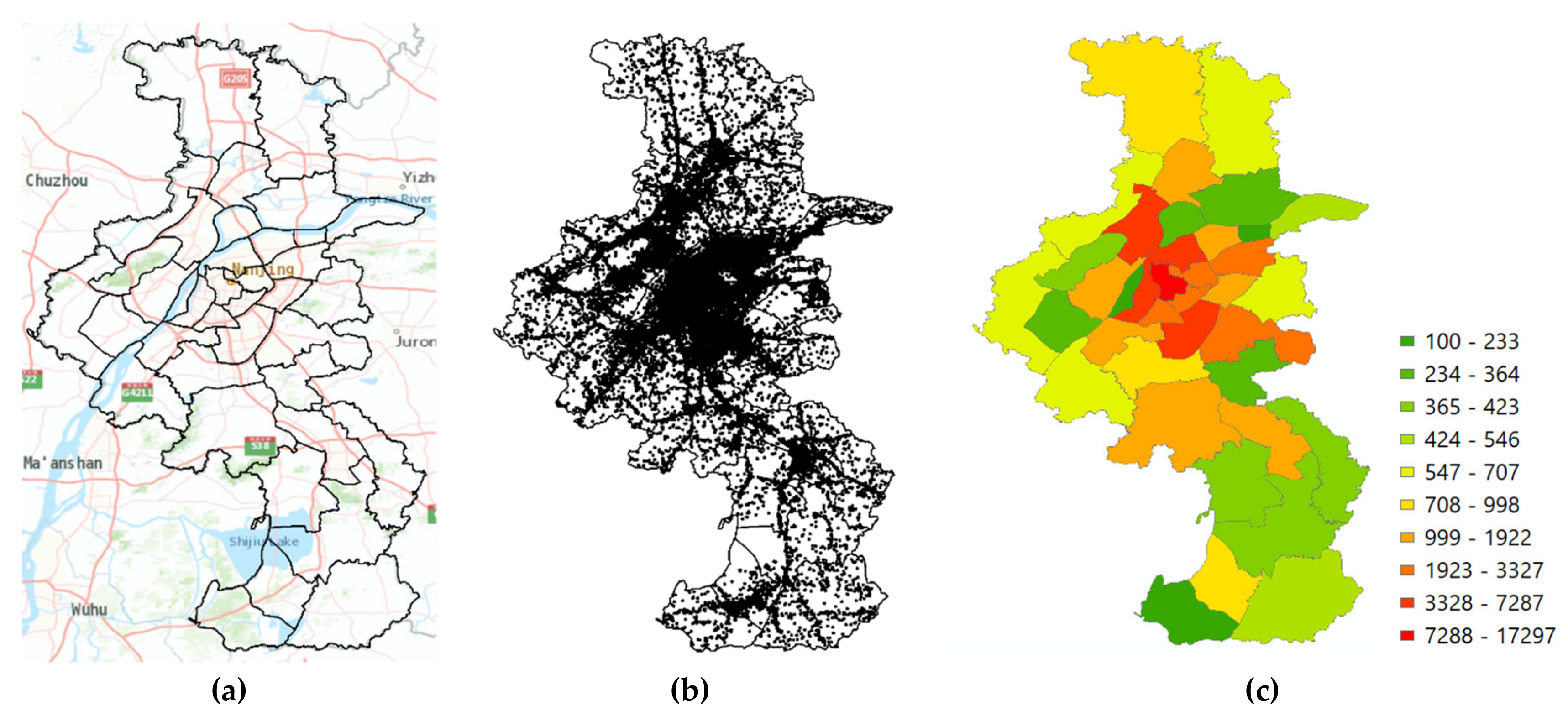
In this research, we have collected mobile phone signaling records from the largest cellular service provider in the city of Nanjing during October, 2017. Figure 1 displays the spatial distribution of the base stations in Nanjing. The city is divided into 38 traffic analysis zones by the Transportation Planning Agency. As indicated in Figure 1, the base stations are more densely distributed in the central area of the city than in the suburban area, which is consistent with the population distribution of Nanjing.

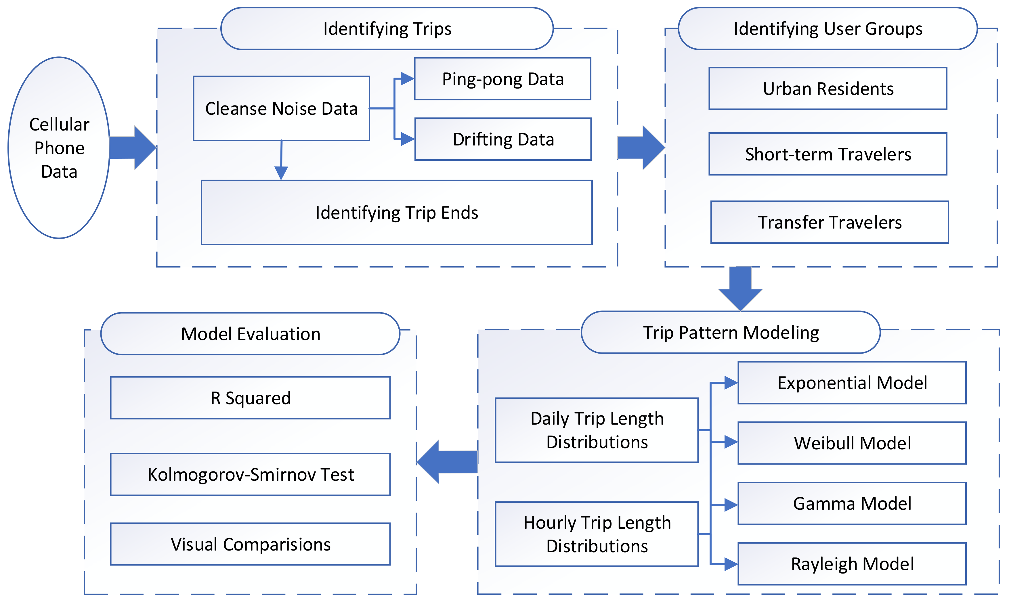
Figure 2 illustrates the methodology framework of the study. Firstly, the cellular phone data was sorted in ordered sequences and then cleansed to eliminate the noise data, including ping-pong and drifting data. Subsequently, trip information was extracted from those signal sequences. In order to examine the heterogeneity in the behavior of different trip makers, we classified the cellphone users into three different groups, namely residents, short-term travelers, and transfer travelers. Then, we tested four different models, including the exponential, Weibull, Gamma, and Rayleigh models in the modeling of daily trip length distribution models and the hourly trip length distribution models for the three groups of cellular phone users. Finally, the R-squared value, Kolmogorov-Smirnov test method, and visual comparison methods were used to evaluate the models.

3.1. Cellular Phone Data

A complete cellular phone signal record contains multiple fields and we only kept the fields related to location information in order to reduce the volume of the original data. The data structure of the cellular phone signal record is: {MSID, Date_Time, LAC,CellID,EventID}. The definitions of each data field are listed as follows:

MSID: The phone number is encoded to protect users’ personal information. This field is unique for each individual user.

Date_Time: The time when the record is generated.

LAC: (Location Area Code): A location area refers to the area where mobile phones can move freely without reporting their location to the cellular service provider. When a cellphone moves out of a location area, a location update event will be triggered. A location area may cover several base station cells.

CellID: The unique ID for a base station cell, a base station cell refers to the service area covered by a base transceiver station (short for base station in the following context). The LAC and the CellID must be used together to uniquely identify a base station cell. The base station cell in the urban area generally covers less than 300 meters in radius range, and the distance between the two base stations in the suburb area may reach more than one kilometer. The spatial resolution can satisfy the traffic demand analysis requirements.

EventID: There are three types of event that can generate a mobile phone signaling record, including a location update, handover and phone calling.

-

Location update: When a mobile phone moves from one location area to another, a normal location update event will be generated. If the mobile phone generates no location update time for a very long time, a periodic location update event will be triggered to confirm the location of the mobile phone. The cycle length of the periodic location update event is about 1 hour.

-

Handover: When the mobile phone is on call and the user is moving from one base station cell to another, a handover event will be triggered to switch the call channel from the original base station to ensure the call quality.

-

Phone calling and messages: When the users make phone calls or send/receive text messages, a phone call event will be generated.

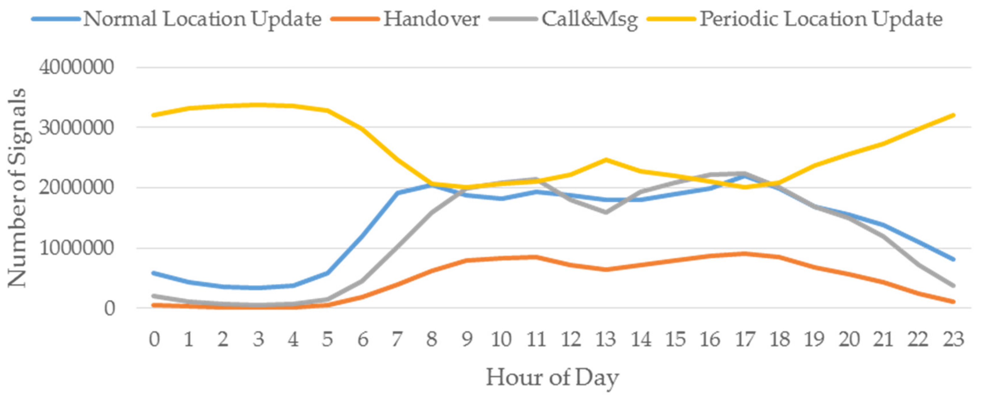
Figure 3 displays the average hourly volume of signaling records during the research period in Nanjing. The number of handover signals and call/message signals both peak at 9:00–11:00 and 16:00–18:00, which coincides with the normal peak traffic hours. The trends of the curves of the normal location update and the periodic location update appear to be opposite, since periodic location update signals are generated when mobile phones stay in the same location update area and no normal location update signal is triggered for one hour.

3.2. Identify Trip Origin-Destination Information using Cellular Phone Data

The responsibility of the cellular phone signaling system is to ensure the quality of the phone calling services, not to locate the accurate real-time position of the users. Due to the complexity of the telecommunication system, the original mobile phone positioning data obtained from the cellular service provider have a substantial amount of redundant data and disturbance data, therefore it is necessary to first filter and eliminate these noise data to improve the data quality. We need a procedure to cleanse the signal records and extract the users’ origin–destination. The method involves the following steps:

(1)

Sorting signal records in ordered sequences: The format of the original signal record is: {MSID, Date_Time, LAC, CellID, EventID} Firstly, we need to map the location of the base station using the LAC and CellID in order to obtain the geocoordinates of the base stations, and then sort each user’s signal records by the Date_Time to obtain each user’s trajectory.

(2)

Cleansing ping-pong signals and drifting signals: Ping-pong signals and drifting signals constitute the two major types of noise data in the users’ trajectory. Typically, the nearest base station to a user would take charge of the users’ phone service. When the workload of the nearest base station is large or the signal is weak, users may be allocated to a farther base station, which forms the drifting signal. In the telecommunicating peak hours, many base stations experience excessive workload, and the users may be switched back and forth between two adjacent base stations, which arouses the ping-pong signal.

Firstly, we need to traverse through the users’ trajectories and calculate the time difference, distance, and speed difference between every two consecutive signal records. Then, we can determine whether the signal is a ping-pong signal or a drifting signal by evaluating these differences.

When the drifting signal occurs, the user is instantaneously switched to a base station far away. Therefore, the speed of two consecutive signal records would be relatively large. If it is greater than the minimum drift speed threshold V1, we can determine that a drifting signal has occurred, and the drifting signal needs to be deleted. The minimum drift speed threshold V1 is recommended to be set to 1.2 times the maximum speed limit of the regional road.

Because most of the ping-pong signal occurs in a short time, it is necessary to set a time threshold, T1. If the difference between a signal record and its previous signal record is greater than the time threshold T1, it is not considered to be ping-pong data. The threshold T1 for filtering ping-pong data is recommended to be 600 s. In order to eliminate all ping-pong signals, each signal record i should be compared with its previous signal record, i–1, and its following signal record i+1. If the previous signal record i–1 and the following signal record i+1 are in the same location, then the signal record i can be determined as ping-pong data and needs to be deleted.

(3)

Identify trip ends: If a user stays in a region with a high density of base stations for a long time, the telecommunication system may randomly switch the base station of the user to nearby base stations in order to balance the telecommunication traffic. Therefore, changes of base stations in a user’s signal sequence may not indicate a trip. To identify a user’s stay area and the duration of the stay, the following method is applied in our study: Select K pieces of signal records in sequence, and set the initial value to K=2, then calculate the coordinates of the center of gravity point C of those K points. If the distance from the K points to the center of gravity point C is less than the threshold C1, then the K records are considered to be a stay rather than a trip. Let K=K+1 and continue the loop, the loop is stopped until the distance from the newly added point to the center of gravity C is greater than C1. The threshold C1 is set to be 500 meters and the maximum value of K is set to 5. A higher K value can increase the accuracy but would increase the complexity of the algorithm.

3.3. Identify Urban Residents, Short-Term Travelers and Transfer Travelers

The urban residents and travelers obviously have different travel behaviors, since urban residents have a fixed home in the city, they would take more routine commuting trips while the trips made by travelers are more diversified. We define “short-term travelers” as the travelers who stay in the city for more than one day while “transfer” travelers don’t stay overnight in the city. Transfer travelers maybe passengers who pass through the city or travelers who return after completing their specific trip purposes. Short-term travelers may be business travelers or tourists who would dwell in hotels. The trip mode preferences and trip length distributions of short-term travelers and transfer travelers may have significant difference. Therefore, we classified urban trip makers into these three categories.

In order to distinguish urban residents, short-term traveler, and transfer travelers, we need to collect and process mobile phone signaling data for several consecutive days, and then count the number of days that mobile phone users appear in the city under study, and divide the users into the three groups according to the proportion of users staying in the research cycle.

In this research, the analysis period is 30 days, and if the user appears less than 1 day, the user is considered to be a transfer traveler. If the user appears more than 1 day but less than 30 × 30%=9 days in the analysis period, the user is regarded as a short-term traveler.

3.4. Trip Length Distribution Model

The trip length distribution model describes the percentages of trips at each separation of trip distances. The most frequently used probability distributions used in trip length frequency distribution models include Gamma, Weibull, Exponential, and Rayleigh distributions.

1. Gamma Distribution

The gamma distribution is a two-parameter continuous distribution with its origin being zero. Functionally it is represented as follows [20,21]:

$$f\left(x\right)=\frac{b}{{\mathrm{b}}^a\mathsf{\Gamma }\left(a\right)}{x}^{a-1}{e}^{-\frac{x}{b}}$$

(1)

where, a refers to the shape parameter, b is the scale parameter, and f(x) refers to the number of occurrence of trips of distance x.

2. Weibull Distribution

The Weibull distribution is generally represented as a three-parameter distribution, similarly to the gamma distribution, it becomes a two-parameter continuous distribution when the origin is zero. For strictly positive values of the shape parameter b and scale parameter a, it is represented as follows [22]:

$$f\left(x\right)=\frac{b}{\mathrm{a}}{\left(\frac{x}{a}\right)}^{b-1}{e}^{-{\left(\frac{x}{a}\right)}^b}$$

3. Exponential Distribution

The exponential distribution is a commonly used distribution in reliability engineering, exhibiting a constant failure rate characteristic with respect to operating time. The exponential distribution is a special case of gamma distribution (obtained by setting a = 1). The exponential distribution is special because of its utility in modeling events that occur randomly over time—it is represented as follows [23]:

$$f\left(x\right)=\frac{1}{\mu }{e}^{-\frac{x}{\mu }}$$

where $\mu$ represents mean trip distance.

4. Rayleigh Distribution

The Rayleigh distribution is a special case of the Weibull distribution. If a and b are the parameters of the Weibull distribution [24], then the Rayleigh distribution with parameter b is equivalent to the Weibull distribution with parameters a = $\sqrt{2}$b and b = 2. The Rayleigh distribution is represented as:

$$f\left(x\right)=\frac{x}{b^2}{e}^{-\frac{x^2}{2b^2}}$$

3.5. Evaluation Methods

The value of the coefficient of determination (R-squared) is used in this research as the primary criterion in evaluating how well the theoretical distributions matched the observed distributions. The R-squared value is calculated using the following equation:

$$R^2=\sum {\left[\frac{\left(x_i-\overline{x}\right)\left(y_i-\overline{y}\right)}{{\sigma }_x\times {\sigma }_y}\right]}^2$$

where $x_i$ refers to the actual observed number of trips at a certain distance i, $y_i$ the number of trips calculated by the model at a certain distance i $, \overline{x}$ is the mean value of $x_i, \overline{y}$ the mean value of $y_i, {\sigma }_x$ the standard deviation of $x_i$, and ${\sigma }_y$ is the standard deviation of $y_i$.

The value of R-squared would fall between 0 and 1. A value of R-squared equal to 1 would imply that the model provides perfect predictions. The closer the value is to one indicates a greater ability to predict.

We use a two-sample Kolmogorov–Smirnov test method(KS test) in order to test whether two datasets belong to the same distribution. The two-sample KS test calculates the absolute distances between the cumulative distribution functions of the distributions of the two datasets. The maximum distance is then plugged into the KS probability function to calculate the probability value p. The test statistic is:

$$D^{*}=\max \left(\left|\widehat{F_1}\left(x\right)-\widehat{F_2}\left(x\right)\right|\right)$$

where $\widehat{F_1}\left(x\right)$ is the proportion of x1 values less than or equal to x and $\widehat{F_2}\left(x\right)$ is the proportion of x2 values less than or equal to x. The lower the probability value p indicates the less likely the two distributions are similar.

In addition, a visual comparison of the actual trip length distribution and the predicted trip length trip distributions would also be used as an auxiliary measure to compare the quality of the models.

4. Results

In this section, we investigated the performance of the four distribution models introduced in the previous section in modeling trip length distributions for various traveler groups, including permanent residents, short-term travelers and transfer travelers in various time periods.

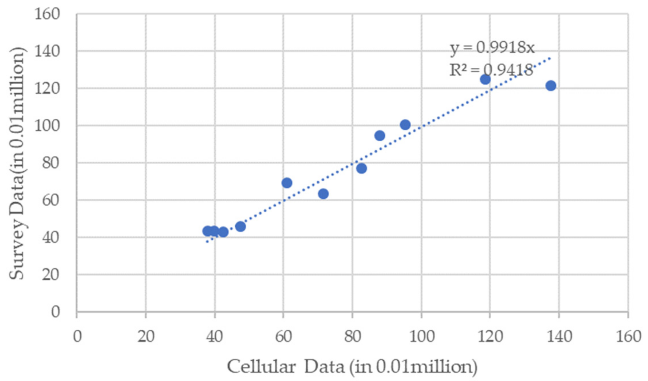
We have analyzed the cellphone signal data for a whole month in October 2016. About 150 million signaling records are processed for each day using the method presented in the previous section on a Hadoop system. We have identified 2.32, 0.664, and 0.193 million average daily resident users, short-term traveler users, and transfer users, respectively. The market penetration rate of the cellular service provider is about 62% in Nanjing and 45% of the users’ cellular records are collected by our system. Therefore, our sample size is about 28% of the population and we need to multiply 1/0.62/0.45 = 3.584 in order to calculate the total population in the city. As indicated in the 2016 survey, there are 8.274 million residents in Nanjing, which is very close to our result, 2.32 × 3.584 = 8.315 million. We also compared the number of residents calculated by the cellular data in each administrative zone with the survey results. As indicated in Figure 4, the maximum error in a zone is about 15%. Although the cellular data tend to underestimate the population, after calibrating the general error is very close to the survey.

Figure 5 displays the number of trips made by residents, short-term travelers, and transfer travelers during the 31 days. As indicated in the figure, residents contribute about half the amount of trips, while short-term travelers constitute more than 30% percent of the total trips, and transfer trips contribute about 10% of the total trips. The figure also suggests that the trip pattern differs significantly from holidays and weekends to normal weekdays, where the period between October 1 and October 7 belongs to the Chinese national holidays. Trips made by the residents are less in the holidays and weekends than in the normal weekdays. The transfer trips are higher in the holidays when short-term traveler trips are more frequent. The difference in short-term trips between holidays, weekends, and normal weekdays is not so significant compared with the other two groups of travelers.

4.1. Daily Trip Length Distribution Models

Firstly, the trips are aggregated by 100 meters of trip distances, and resulted in 500 groups of trip distances in the range of 0–50 km. Then, the trip length distributions of the various population groups are compared using the Kolmogorov–Smirnov method in order to test whether they follow the same distribution statistically.

Table 1. Kolmogorov–Smirnov Test Statistics for the Trip Length Distributions of Various Groups.

Trip Maker Group	KSstat	p	h
Resident vs. Short-term Traveler	0.154	1.17E-05	1
Resident vs. Transfer Traveler	0.306	4.37E-21	1
Short-term Traveler vs. Transfer Traveler	0.266	4.88E-16	1

displays the KS test statistics of the pairwise comparison of the trip length distributions of the three population groups at the 5% significance level, the p-value of all the tests are close to 0 and h = 1, which indicates that the null hypothesis—that the trip distributions are from the same continuous distributions—is rejected.

Figure 6 illustrates the trip length distribution characteristics of various population groups. As shown in Figure 6, the trip distances travelled by residents tends to be longer than transfer travelers and short-term travelers. The trip distances of short-term travelers are the lowest among all three population groups.

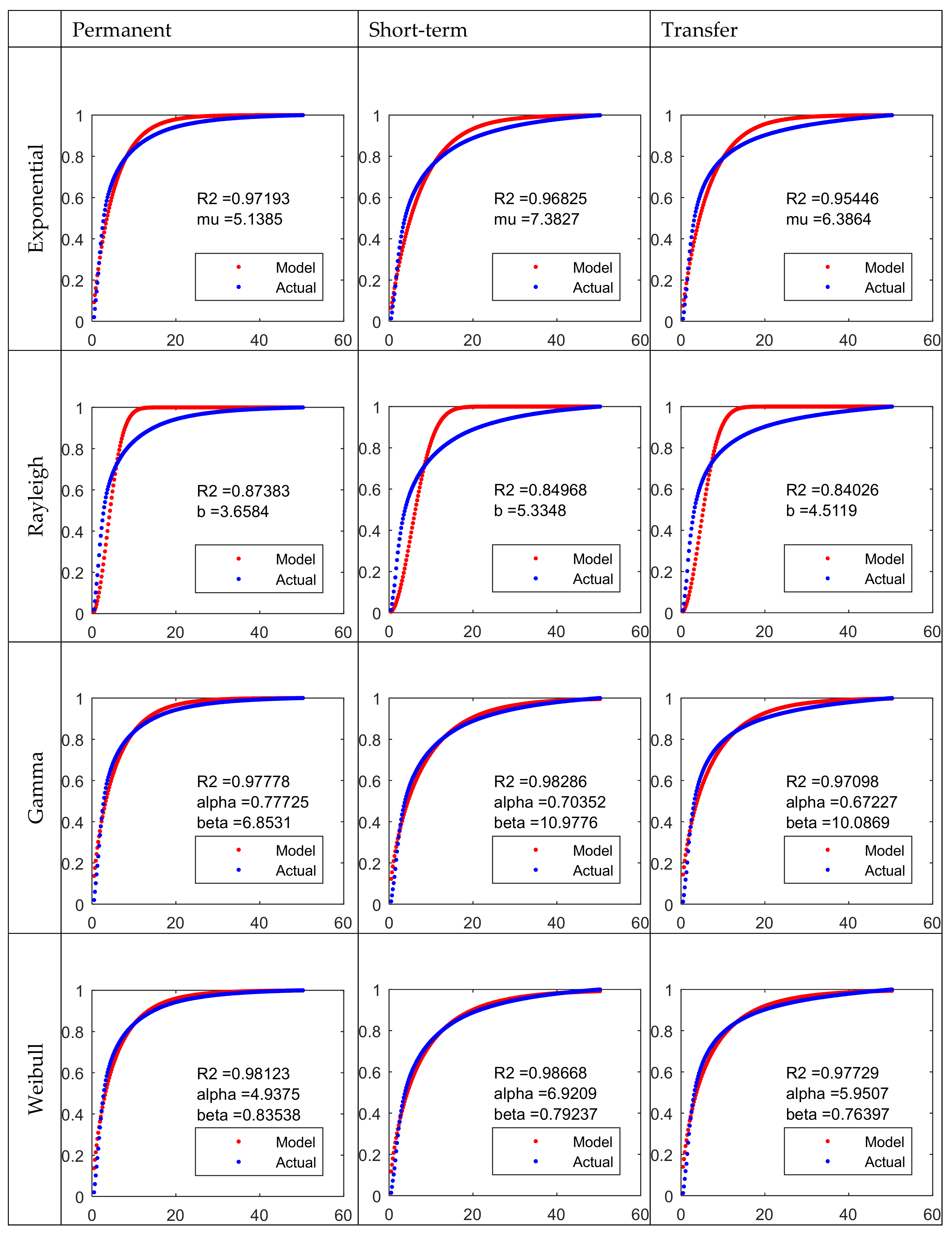
As indicated in Table 1, as well as Figure 5 and Figure 6, the trip characteristics of the residents, short-term travelers, and transfer travelers differ significantly in terms of travel time and travel distances. Therefore, when modelling the trip length distribution characteristics, the heterogeneity in the travel behavior of different population groups should be considered. Therefore, we built separate trip length distribution models for each type of population group. We tested the four most popular models, including the exponential model, the Rayleigh model, the gamma model and the Weibull model in order to compare and select the best one—the results are listed in Figure 7.

As shown in Figure 7, the gamma and Weibull model methods outperform the exponential and Rayleigh methods in estimating the trip length distributions of all three population groups. The advantage in estimation accuracy could be attributed to the extra number of parameters in the gamma and Weibull model methods. For the two parameter models, the Weibull model method has slightly better advantage while in the one parameter models, the exponential model method is obviously better than the Rayleigh model method. In conclusion, if only one model parameter is allowed in the daily trip length distribution model, the exponential model method should be used, and if the number of model parameters is not so sensitive, the Weibull model method is recommended.

4.2. Within-Day Trip Distances Distribution Models

From the analysis in the previous section, the trip patterns of the residents, short-term travelers, and transfer travelers vary with different time periods in a day. In traditional transportation planning applications, the daily trip distance distribution model is fundamental in the gravity model [25,26]. When it comes to dynamic trip demand estimation, the time-varying property of the trip length function should be taken into account. This section presents the within-day trip distance distribution models.

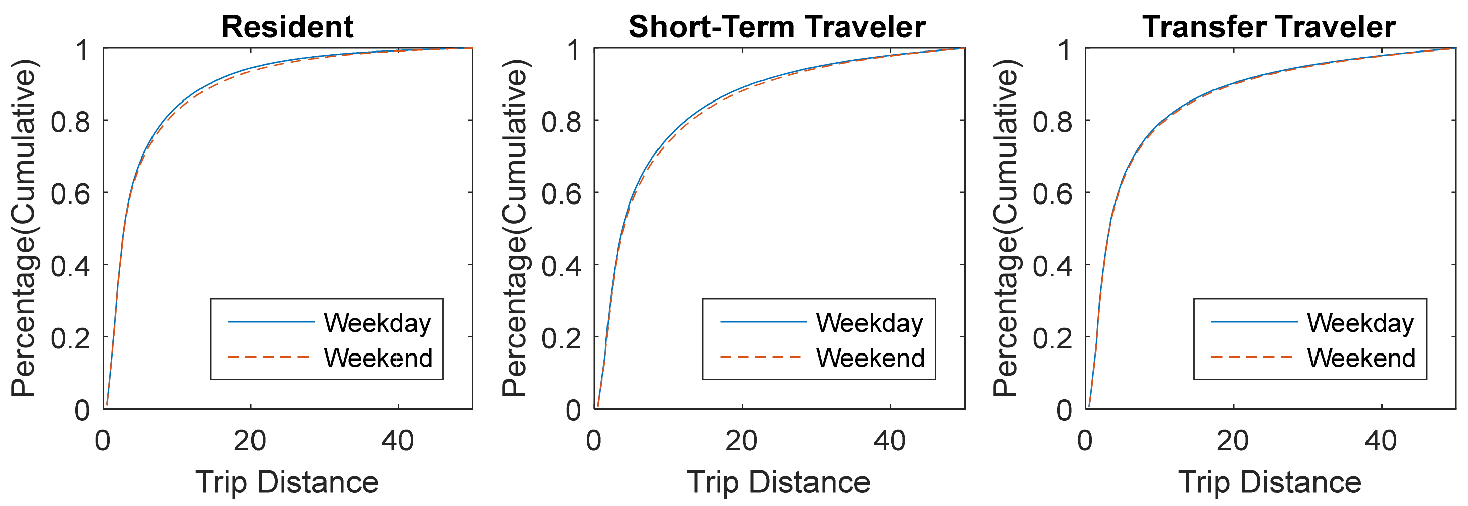
Firstly, we compared the weekday and weekend travel patterns in Figure 8 to find that residents and short-term travelers tend to travel more on weekdays than on weekends, while for transfer travelers the difference is not significant.

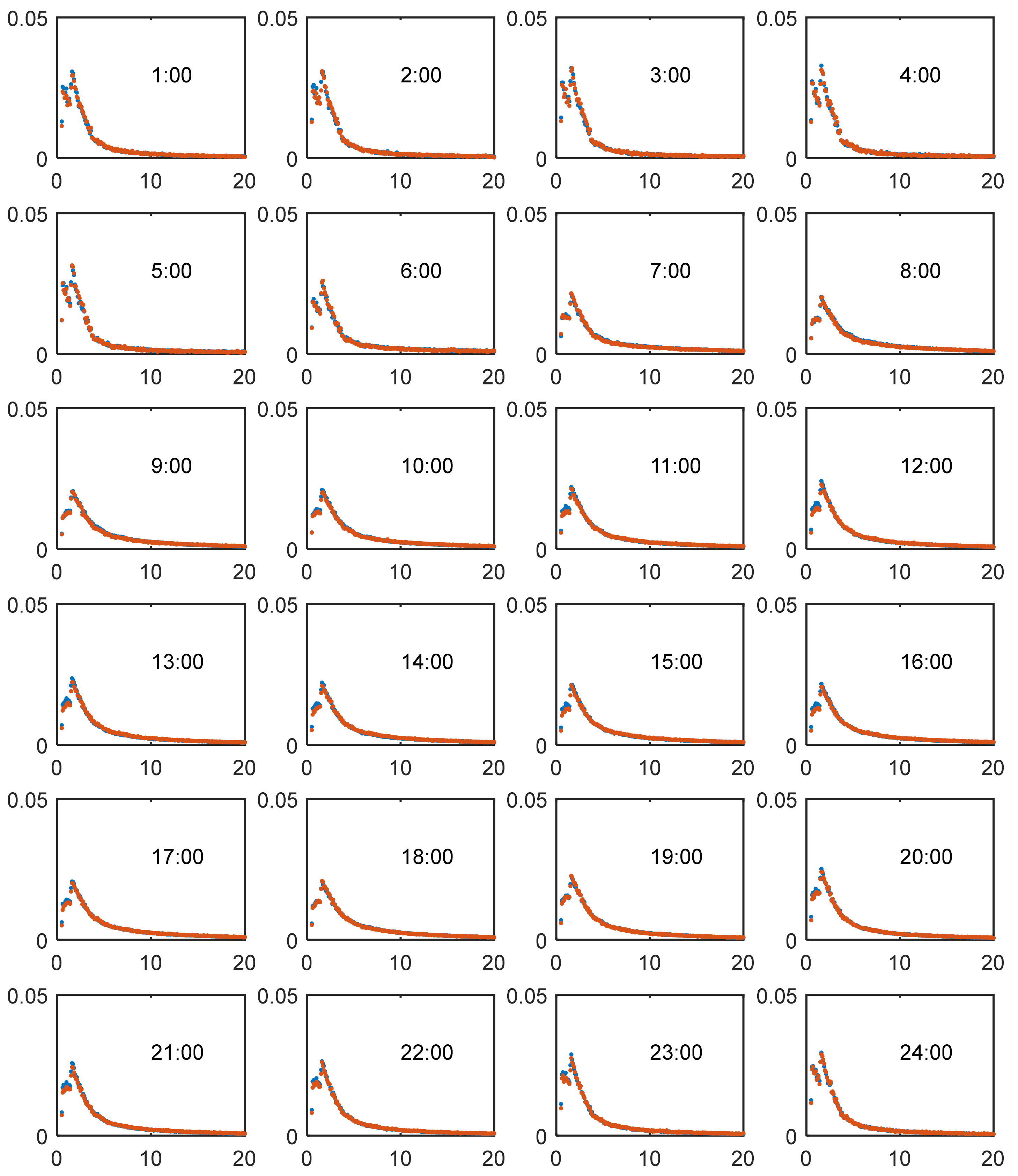
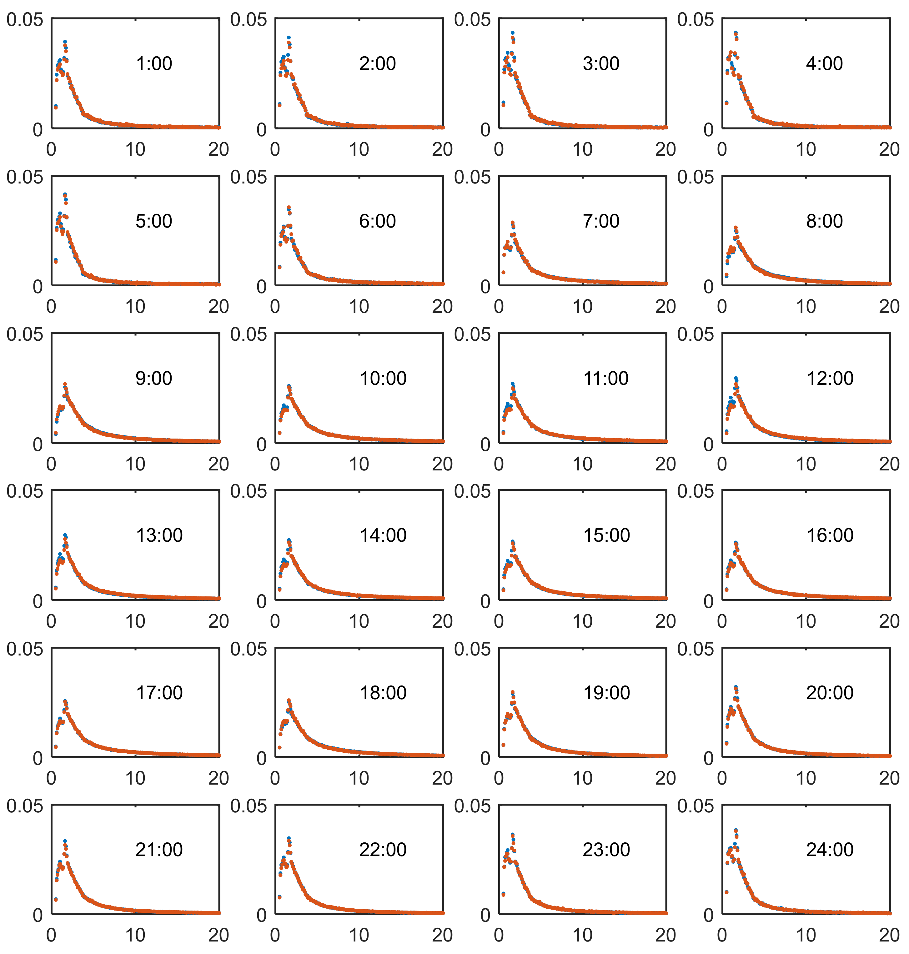
In order to examine the fluctuation in the hourly trip length distributions, we plotted the hourly trip length distribution of the residents in Figure 9 (the hourly trip distribution of the short-term travelers and transfer travelers can be found in Figure A1 and Figure A2 of the Appendix A). The red dots refer to the weekday trips, while the blue dots represent the weekend trips. As indicated in Figure 9, the trip length distribution pattern can be approximately divided into two categories. In the late night and early morning, trips tend to be shorter—meanwhile, in the daytime, there are longer trips.

Although developing separate models for each hour may be more accurate numerically, the complexity of the models would bring difficulty in practice. We adopted the hieratical agglomerative clustering method to group similar hours, so the similar hours in the same group could share the same trip length distribution model. The hourly trip length distribution model can be classified into six scenarios according to the population group (resident/short-term traveler/transfer traveler) and by weekday/weekend. Dendrograms of the hourly trip length distribution of the six scenarios are plotted in Figure 10. For all of the six scenarios, the hours can obviously be classified into two groups: the morning hours group and the night hours group, but there are slightly differences in the division of the hours. For residents, the hours in the weekdays are divided into morning hours (7:00–21:00) and night hours (1:00–6:00; 22:00–24:00), the hours in the weekends are divided into morning hours (7:00–22:00) and night hours (1:00–6:00; 23:00–24:00). For short-term travelers, the hours in the weekdays and weekends are both divided into morning hours (8:00–19:00) and night hours (1:00–7:00; 20:00–24:00). For transfer travelers, the hours in the weekdays are divided into morning hours (8:00-19:00) and night hours (1:00–7:00; 20:00–24:00), and the hours in the weekends are divided into morning hours (7:00–22:00) and night hours (1:00–6:00; 23:00–24:00).

In order to test whether the division of the six scenarios is reasonable, we use the KS method to test the differences in the distributions for various weekday/weekend and morning/night combinations. The test results are displayed in

Table 2. Kolmogorov–Smirnov Test Statistics for the Various Hourly Trip Length Distributions.

Group	Time Period	ks2stat	p	h
Permanent	Weekday Morning vs. Weekday Night	0.482	1.09E-51	1
Permanent	Weekend Morning vs. Weekend Night	0.516	3.57E-59	1
Permanent	Weekday Morning vs. Weekend Morning	0.27	1.64E-16	1
Permanent	Weekday Night vs. Weekend Night	0.252	1.95E-14	1
Short-Term	Weekday Morning vs. Weekday Night	0.474	5.33E-50	1
Short-Term	Weekend Morning vs. Weekend Night	0.462	1.60E-47	1
Short-Term	Weekday Morning vs. Weekend Morning	0.368	2.63E-30	1
Short-Term	Weekday Night vs. Weekend Night	0.364	1.16E-29	1
Transfer	Weekday Morning vs. Weekday Night	0.568	1.30E-71	1
Transfer	Weekend Morning vs. Weekend Night	0.69	1.78E-105	1
Transfer	Weekday Morning vs. Weekend Morning	0.708	4.99E-111	1
Transfer	Weekday Night vs. Weekend Night	0.536	8.12E-64	1

, and indicate that all the pairwise comparisons are not in the same continuous distribution at the 5% significance level. Therefore, the division of the six scenarios is plausible and we can build separate trip length distribution models for each scenario.

Similar to the process to obtain daily trip length distribution models, we compared the four models, including the exponential model, the Rayleigh model, the gamma model, and the Weibull model to compare and select the best within-day trip length distribution model for the forementioned 12 conditions. The R-squared values of the results of these four models under 12 conditions are listed in

Table 3. R-Squared Values of the Trip Length Distribution Models.

			Exponential	Gamma	Rayleigh	Weibull
Resident	Weekday	Night 1–6, 22–24	0.96271	0.9631	0.89532	0.96508
Resident	Weekday	Morning 7–21	0.97611	0.98099	0.87906	0.98386
Resident	Weekend	Night 1–6, 23–24	0.95826	0.95969	0.88815	0.96294
Resident	Weekend	Morning 7–22	0.9714	0.97929	0.86747	0.98291
Short-term	Weekday	Night 1–7, 20–24	0.95198	0.97281	0.83113	0.97907
Short-term	Weekday	Morning 8–19	0.97359	0.98523	0.85847	0.98841
Short-term	Weekend	Night 1–7, 20–24	0.94972	0.97239	0.82586	0.9787
Short-term	Weekend	Morning 8–19	0.97362	0.98594	0.85561	0.98888
Transfer	Weekday	Night 1–7, 20–24	0.93683	0.95432	0.82974	0.96362
Transfer	Weekday	Morning 8–19	0.96164	0.97565	0.84823	0.98084
Transfer	Weekend	Night 1–6, 23–24	0.91145	0.9341	0.80634	0.94751
Transfer	Weekend	Morning 7–22	0.9584	0.97366	0.84388	0.9793

. Similarly, the Weibull model is found to have the best accuracy and, for one-parameter models, the exponential model produces the better results. The model parameters of the Weibull model and the exponential model are listed in

Table 4. Parameters of the Weibull-based Trip Length Distribution Models.

Population Group	Period		Alpha	Beta
Resident	Weekday	Morning	3.4915	0.90081
Resident	Weekday	Night	5.1596	0.84959
Resident	Weekend	Morning	3.6428	0.86553
Resident	Weekend	Night	5.3778	0.82268
Short-term	Weekday	Morning	5.8899	0.74902
Short-term	Weekday	Night	7.1813	0.81181
Short-term	Weekend	Morning	6.087	0.74422
Short-term	Weekend	Night	7.5603	0.81173
Transfer	Weekday	Morning	4.8515	0.73443
Transfer	Weekday	Night	6.3636	0.7834
Transfer	Weekend	Morning	4.4437	0.6935
Transfer	Weekend	Night	6.285	0.77502

.

5. Conclusions

This paper explores trip length distribution functions for heterogeneous population groups utilizing cellphone signaling data at a large-scale (5 million individuals). We investigated the feasibility of using four models, including the exponential model, the Weibull model, the Rayleigh model, and the gamma model, in modeling the daily trip length distributions for heterogeneous population groups. We found that the trip distributions are different for the three distinct groups of residents, namely residents, short-term travelers, and the transfer travelers. In addition, we investigated the statistical variations of trip distribution models caused by different time periods and found that the trip distributions for the daytime and nighttime are distinct. We also found differences in the trip distribution patterns between weekdays and the weekend. In order to improve the accuracy of the models, we proposed a clustering method to group different hours in a day, and proposed separate trip length distribution models for different partitions of the day for each traveler group. Our results suggested that the gamma distribution performs well in trip length distribution modeling under various conditions, and the exponential model is also suitable for trip length distribution models when the number of model parameters is sensitive in application.

Our work extends the traditional trip length distribution method with a new perspective on the heterogeneity of the traveler group and the different time periods, and provides an important decision-making basis for urban transportation planning. However, we still recognize two major drawbacks that arise while using cellular phone data to model urban mobility patterns. Firstly, the market share of the mobile phone operator may be uneven for different parts of the city, which can affect the statistical results. Other data sources, such as loop detector data or video surveillance data, could be used to calibrate the market penetration rate to improve the accuracy. Secondly, cellular phone data could not provide users’ personal social-economical information due to privacy issues, which is indispensable when analyzing the impact of individuals’ travel behavior.

Addressing these aforementioned limitations will be part of our future work. In addition, the study of trip length distribution characteristics also has the following applications and research prospects.

(1) It can be used as the impedance function of the trip distribution model to improve the transportation planning procedure to obtain origin–destination matrices of better precision for residents, short-term travelers, and transfer travelers. The results could provide supportive information for transportation agencies in the traffic management procedure, such as traffic control in holidays and special events and policy making in license plate number restrictions, etc.

(2) When planning for new roadways, the trip volume and the travel probability under a certain trip distance can be used as key indicators in determining the road function class.

(3) This method could also be applied in other cities where cellular data is available to explore the trip length distribution pattern in cities of various gross domestic products, populations, area size, and so forth, and identify the influencing factors.