Abstract
An effective way to optimize traffic structures is by changing travel costs, thereby moving travelers from private transportation to public transportation. However, according to the existing studies, the traveler will not transfer from one mode to another unless the change in travel utility is greater than the indifference threshold. Therefore, the “indifference threshold” is one of the most important factors influencing a traveler’s choice of behavior. This study defines the “indifference threshold” as the traveler’s sensitivity to changes in travel utilities. In the framework of the theory of planned behavior (TPB), a structural equation model (SEM) considering the indifference threshold is established to analyze a traveler’s mode choice behavior. The analysis results showed that a travelers’ sensitivity to changes in travel utilities has the greatest impact on mode-choice behavior intentions and mode choice behavior. Perceptual behavior control has the strongest influence on travel choice behavior. In addition, in order to further explore the heterogeneity of a traveler’s behavior, the travelers were subdivided into four types, by establishing a latent class model (LCM) considering the indifference threshold. Finally, different traffic management suggestions are proposed for different types of travelers.
1. Introduction
Reducing the travel cost of public transportation (such as building a bus lane) or increasing the travel cost of private transportation (such as increasing the parking fees in central areas of the city) are effective ways to optimize traffic structures, to promote sustainable transportation development, and to help travelers transfer from private transportation to public transportation [1]. However, according to the satisfactory decision theory proposed by Simon [2] and the related research of many subsequent scholars [3,4,5,6,7,8,9,10,11], only when a change in travel utility is greater than a certain threshold (i.e., the indifference threshold) is it possible for the traveler to transfer from one mode to another. Therefore, the “indifference threshold” is one of the important influencing factors for a traveler’s choice behavior, and it is also one of the factors that influences whether a traffic demand management policy can be effectively implemented [12].
The concept of the indifference threshold stems from psychology’s experiments on perceived indifference. As reported in Guilford [13], the concept of the perception threshold was first proposed by Herbart. Later, Weber came up with a concept called “just noticeable difference”. The classical psychology of Fechner, Miller, and Wundt focused on how this threshold was determined. Classical economists have also proposed the concept of “indifference”. Slutsky first used the indifference curve to analyze a consumer’s choice behavior. Simon [2] proposed a satisfactory decision-making criterion, arguing that individuals follow satisfaction criteria rather than optimal criteria when making decisions. Quandt [14] proposed the concept of the indifference band of commodity utility. Georgescu–Roegen [15] introduced the concept of threshold into the theory of consumer choice, suggesting that consumers will not change their choices unless the utility difference exceeds a certain “necessary minimum”. In 1977, Krishnan [3] introduced the concept of the indifference threshold into the study of travel behavior in the field of transportation. He defined the indifference threshold as the “minimum perceivable differences” between the utilities of two alternatives and proposed a minimum perceivable difference (MPD) model. Then, Lioukas [4] extended Krishnan’s binary theory to multiple alternative situations using a multinomial logit model. Later, the “indifference threshold” was gradually applied to the study of traffic problems, such as mode choice behavior, departure time choice behavior, route choice behavior, the optimal transit fare, and the day-to-day evolution of traffic flow. For example, Mahmassani et al. [5,6,7] introduced the concept of the indifference threshold into the bottleneck model, and studied the problem of departure time choice considering the travelers’ bounded rationality. Di et al. [8] studied the change of a traveler’s route choice behavior after adding a new path to the original road network. The analysis results show that travelers will move to a new path only if using a new path can save travel time beyond a certain threshold. Carrion and Levinso [9] studied the traveler’s route choice behavior based on GPS data. They found that a threshold exists in the route choice decisions of travelers. When the threshold exceeds the travel time of a certain road, travelers will abandon this road and move to another one. Tao and Hongzhi [10] assumed that decision-makers could make accurate judgments when the utility difference between alternatives is large enough. However, when the utility difference between alternatives is less than a certain extent, the decision maker will choose the path according to his preference (or choose randomly). Next, a boundedly rational binary logit (BRBL) model was presented. Recently, Xinjie et al. [11] extended this model and proposed the boundedly rational nested logit (BRNL) model.
In summary, the existing research in the field of transportation mostly considers the influence of the “indifference threshold” from the perspective of travel utility. However, from the view of psychology, the “indifference threshold” can be understood as a traveler’s sensitivity to changes in travel utility. Many scholars have studied the influence of psychological factors on travel behavior [16,17,18,19]. For example, Christian et al. [20] established a structural equation model based on the theory of planned behavior, and discussed the influence of psychological factors such as “behavioral intention”, “subjective norms”, “behavioral habits”, and “external environment” on environmentally friendly travel behaviors. Lei et al. [21] built an unsafe cycling behavior model for cyclists based on planned behavior theory. Jian [22] analyzed the travel psychology of residents in public transportation, and proposed that the characteristics of travelers would indirectly affect the travel behavior through the psychological latent variables of the planned behavior theory. Based on the original planned behavior theory, Peng [23] introduced descriptive norms and latent variables of behavioral habits, and explored the influences of psychological factors on behaviors and intentions in the selection of inter-city travel modes in the metropolitan area, by establishing a regression model.
In recent years, the multi-criteria decision making (MCDM) approach have been adopted by some studies to solve transportation problems. For example, Duleba and Moslem [24] introduced a decision making model combining analytic hierarchy process (AHP) with Kendall rank correlation and an extra level of stakeholder significance in the decision. They examined the preferences of different stakeholder groups (passengers, potential passengers, and local government) and created an acceptable coordination for an ultimate, sustainable decision. Ghorbanzadeh et al. [25] applied an interval analytic hierarchy process (IAHP) dealing with the inconsistencies and uncertainties of users responses, by comparing the results of passengers to reference stakeholder groups. However, these studies on the impact of psychological factors on travel behaviors have rarely considered the impact of travelers’ sensitivities to changes in travel utility.
In addition, scholars have also found that there is significant heterogeneity among travelers’ choice behaviors [26,27]. Therefore, some studies have applied the latent class model to analyze the heterogeneity of travelers. Latent class analysis comes from the concept of factor analysis put forward by Spearman in 1904 [28]. As a result of Joreskog and Lazarssfled, and Henry’s subsequent contributions [29], latent class models have become widely used. The application of this model in the traffic field mainly focuses on traffic behavior analysis. For example, Greene [30] compared the latent class model with the mixed logit model. The results showed that the latent class model had the advantage of semi-parameterization, which enables researchers to avoid making too strong conditional assumptions about the distribution of individual heterogeneity. Wen et al. [31] used the latent class model to study the preference of passengers to choose international airlines, and divided passengers into four categories.
To sum up, studies about the impact of psychological factors on travel behaviors and the classification of travelers have rarely considered the impact of the “indifference threshold of the change in travel utility” on travelers’ behaviors. Therefore, this study defines the “indifference threshold” as a traveler’s sensitivity to changes in travel utility. Based on the framework of the theory of planned behavior (TPB), “the sensitivity to a change in travel utility” is considered to be a psychologically influencing factor of travel behavior. Based on the data of the travel behavior survey, the structural equation model (SEM) considering the indifference threshold was established, and the influence factors of travelers’ choices between private transportation and public transportation were analyzed. In addition, in order to further explore the heterogeneity of travelers’ mode choice behaviors, travelers were subdivided into different types by establishing a latent class model considering the indifference threshold. Finally, different traffic management suggestions are proposed for different types of travelers.
The remainder of this paper is organized as follows: The next section introduces the research framework and research methods. Section 3 describes the data collection and analysis. The model estimation and subdividing results are presented in Section 4. Section 5 elaborates on the conclusions of the present research and proposes corresponding measures and suggestions, as well as future research work.
2. Methodology
2.1. Model framework
Based on the existing research, this paper defines the indifference threshold as follows:
Definition 1: “Indifference threshold” refers to the change in travel utility that enables a traveler to move from one travel mode to another. That is, only when the change in travel utility is greater than the indifference threshold will travelers move from their current travel mode to another. The indifference threshold represents the degree of the travelers’ sensitivity to changes in the utility of their travel modes. The smaller the indifference threshold is, the higher the traveler’s sensitivity is.
This study considers the influence of a “travelers’ sensitivity to the change in the utility of travel mode” within the framework of the classic theory of planned behavior (TPB). Based on the survey data of travel behavior, the structural equation model of travel mode choice with the indifference threshold is established, and the psychological factors of travelers when they choose two kinds of travel modes (private transportation and public transportation) are analyzed. In addition, in order to further explore the heterogeneity of the travelers’ mode choice behaviors, the travelers are subdivided into different types by establishing a latent class model considering the indifference threshold. The framework of the models is shown in Figure 1. According to the theory of planned behavior (TPB), behavior is directly affected wholly or partly by intention, attitude, subjective norm and perceived behavior control. Based on the TPB, “the sensitivity to a change in travel utility” is considered to be a psychological factor of travel behavior, and a theoretical model of the relationship between psychological factors and behavioral intentions and behaviors was constructed in this paper, as shown in the first part of Figure 1. The constructed model includes five latent variables: attitude (ATT), subjective norm (SN), perceived behavior control (PBC), sensitivity to change in travel utility (SEN), and behavior intention (BI). Among them, BI is an intermediary variable, and the result of behavior is whether to choose public transportation. Based on the analysis of the relationship between psychological factors and mode choice intention and behavior, the heterogeneity of travelers’ behavioral intention and preferences were further explored, and the latent class model was used for tourist segmentation, as shown in the second part of Figure 1. This paper comprehensively considers the combination of personal attributes, psychological factors, and sensitivity to change in travel utility, to carry out segmentation research. Suppose that there is a potential variable X that represents travelers’ preferences for different travel modes. Obviously, each traveler has different preferences, however, travelers with similar preferences can be grouped into one category. Therefore, a latent class model is established in this paper, and the latent variable is determined to obtain the final number of categories.
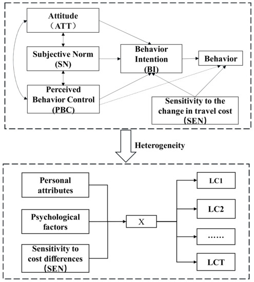
Figure 1.
The model framework.
2.2. The Structural Equation Model
Structural equation modeling (SEM) can transform potential variables, such as attitude, into statistical models [32]. SEM is a data statistical method used to analyze the relationship between observable variables and potential variables, as well as the internal relationship between potential variables. SEM has not only been widely used in the social sciences but also in the study of travel behaviors [33,34]. Compared with other known techniques for applying latent variables, e.g., principal component analysis (PCA), SEM is more suitable for the objective of this study because PCA assumes the existence of the latent variables, yet cannot define them, and the latent variables are a priori well defined in SEM. SEM includes a measurement equation and a structural equation. The measurement equation is used to describe the relationship between explicit variables and latent variables, and the structural equation is used to describe the internal relationship between the latent variables. The expressions are as follows:
Equation (1) is the measurement model of the exogenously observed variables, where is a vector made up of exogenous variables, represents the factor loading matrix of in , is a vector composed of exogenous latent variables, and represents the measurement error vector.
Equation (2) is the measurement model of the endogenous variables, where is a vector of the endogenous variables, represents the factor loading matrix of in , is a vector composed of endogenous latent variables, and represents the measurement error vector.
Equation (3) is the structural model that is mainly used to verify the causal relationship between factors, where is the coefficient matrix, which represents the interaction between the endogenous latent variables, is the coefficient matrix, which represents the influence of each exogenous latent variable on each endogenous latent variable, and is the residual vector of the structure equation.
In this model, the selection of observation variables corresponding to attitude, subjective norms, perceptual behavior control, and travel intentions is shown in Table 1.

Table 1.
Variables in the model.
In this study, SEM was selected to analyze the relationship among variables of the travel mode choice behavior within the theoretical framework of planned behavior. According to the aforementioned theoretical framework of planned behavior, considering the indifference threshold, the following assumptions were proposed for the model:
Hypothesis 1 (H1).
The attitude is positively correlated with the behavioral intention of travel mode choice.
Hypothesis (H2).
The subjective norms are positively correlated with the behavioral intention.
Hypothesis (H3).
The perceived behavioral control is positively correlated with the behavior intention.
Hypothesis (H4).
The perceived behavioral control is positively correlated with the behavior.
Hypothesis (H5).
A traveler’s sensitivity to changes in travel utility is positively correlated with the behavioral intention.
Hypothesis (H6).
A traveller’s sensitivity to changes in travel utility is positively correlated with the travel mode choice behavior.
Hypothesis (H7).
The behavioral intention is positively correlated with the behavior of mode choice.
Hypothesis (H8).
The perceived behavioral control is positively correlated with their sensitivity to changes in travel utility.
2.3. Latent Class Model
When studying the mode choice behavior of travelers, the individual attributes and psychological factors of different travelers affect their preference of mode choice. Suppose there is a potential variable X that represents travelers’ preferences for different travel modes. Obviously, each traveler has different preferences, however, travelers with similar preferences can be grouped into one category. Although it is difficult to measure individuals’ travel preferences directly, it can be seen from the above analysis that there is a complex statistical correlation between traveler preference and traveler attributes, attitudes, subjective norms, perceptual behavior control, sensitivity to utility difference between modes, and other psychological factors. Therefore, a traveler’s attributes, psychological factors, and sensitivity to the utility difference between modes can be taken as explicit variables to establish a latent class model, as well as to further subdivide travelers into different categories and explore the heterogeneity of traveler mode choice behaviors.
Assuming that there are three explicit variables A, B, and C in the model, the mathematical expression of the latent class model (LCM) is:
subject to:
where represents the joint probability of the LCM. is the probability that the observation data belongs to a specific latent class t (t = 1, 2, 3, …,T) of a latent variable X, (that is P (X = t), t = 1, 2, …,T); is the conditional probability that an observation has response i (i = 1, 2, …, I) to the manifest variable A given that the observation is in latent class t; is the conditional probability that an observation has response j (j = 1, 2, …, J) to the manifest variable B, given that the observation is in latent class t; is the conditional probability that an observation has response k (j = 1, 2, …, K) to the manifest variable C, given that the observation is in latent class t.
These conditional probabilities can be used to illustrate the relationship between each latent class and explicit questions, which can help the researcher to explain the content and nature of each latent class. In each latent class, a large conditional probability value indicates that the latent variable has a strong influence on the explicit variable.
In LCM, the maximum likelihood method is mainly used to solve the model. According to the number of classes, the joint probability, latent class probability, and conditional probability of each class are calculated separately [28]. LCM fitness test methods mainly include likelihood ratio chi-square statistics, AIC (Akaike information criterion), BIC (Bayesian information criterion), entropy, and significance level to comprehensively evaluate the accuracy of the classification model. The number of classes is increased one by one from one class, and the value of the test parameters corresponding to each class is compared.
3. Data Collection and Analysis
Data collection in this study was done in the form of a network questionnaire. The survey was conducted in July 2019 and lasted for two weeks. The respondents satisfied the following four conditions simultaneously: (1) The respondent works in Beijing; (2) the respondent’s family has at least one car; (3) the respondent has a driver’s license; (4) the respondent used to travel in the subway in Beijing.
The questionnaire consists of three parts: (1) respondents’ socioeconomic attributes; (2) public transportation travel scale information; and (3) travelers’ sensitivity to the change in travel utility. The second part of the scale is mainly used to measure the psychological variables of travel mode choice behavior within the framework of planning behavior theory. Four basic variables, ATT, SN, PBC, and BI, were constructed in TPB using the Likert five-level scale. The problem setting refers to Table 1. The options in the scale are “strongly disagree”, “disagree”, “general”, “agree”, and “strongly agree”, with values ranging from 1 to 5. The third part sets the scenario questions. The respondents were requested to answer whether they would switch from private transport to public transport if the utility of private transport, such as the parking fee or travel time, increased.
3.1. Descriptive Statistical Analysis
In total, 242 questionnaires were sent and recovered. Among them, 212 questionnaires were valid, with a validity rate of 87.6%. As shown in Table 2, among the valid questionnaires, 50.5% were male and 49.5% were female. For age, 31–40 years old accounted for 65.1% of the total; employees of enterprises accounted for the greatest number, accounting for 57.5%, followed by employees of government offices/public institutions, accounting for 18.4%. The education level was mainly undergraduate, accounting for 43.4%, followed by graduate and junior college, accounting for 28.8% and 22.6%, respectively. Personal monthly income of less than 4000 accounted for 13.2%, 4000 to 10,000 accounted for 50.5%, and 10,000 or more accounted for 36.3%. The majority of the families include three or more residents, accounting for 84%.
Table 2.
Descriptive statistical analysis of the valid samples.
The survey measures travelers’ sensitivities to changes in travel utility from two dimensions: time-cost and expense-cost. According to the respondents’ answers, it can be seen that when only the time- or expense-cost of a certain travel mode is changed, and the other conditions remain unchanged, the change in cost that can facilitate a mode shift (i.e., the indifference threshold) is different for different travelers. That is, different travelers have different levels of sensitivity to changes in travel cost. As shown in Table 3, according to the respondents’ answers, we divided the travelers into three categories through the simplest cluster analysis: High sensitivity to a change in travel cost, neutral sensitivity to a change in travel cost, and low sensitivity to a change in travel cost.
Table 3.
Survey results on sensitivity to changes in travel cost.
3.2. Cross-Analysis of Personal Attributes—Sensitivity to Changes in Travel Cost
We analyzed the relationship between individual attributes and sensitivity to changes in travel cost by crosstab.
3.2.1. Analysis of the Sensitivity of Travelers of Different Genders to Changes in Cost
The sensitivity of travelers of different genders to cost change is shown in Figure 2 and Figure 3. According to the survey results, female travelers are the most sensitive to changes in time-cost among respondents, while sensitivity to changes in the expense-cost of different genders is basically the same.
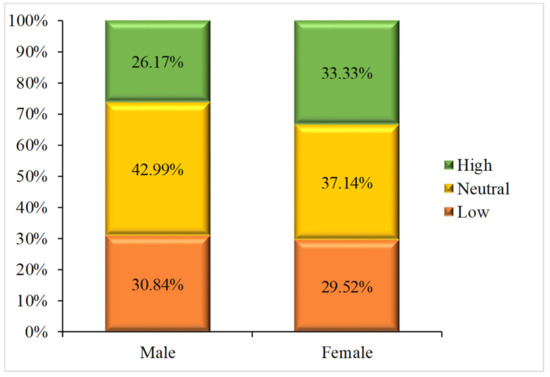
Figure 2.
The sensitivity of travelers of different genders to changes in time-cost.
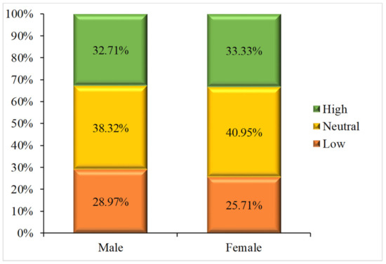
Figure 3.
The sensitivity of travelers of different genders to changes in expense-cost.
3.2.2. Analysis of the Sensitivity of Different Aged Travelers to Changes in Travel Cost
The sensitivity of travelers of different ages to changes in travel cost is shown in Figure 4 and Figure 5. According to the survey results, travelers aged 18 to 30 have the highest sensitivities to changes in time-cost and expense-cost, followed by travelers aged 31 to 40. Conversely, travelers aged 41 to 60 have the lowest sensitivities.
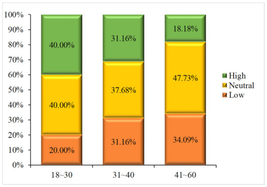
Figure 4.
The sensitivity of travelers of different ages to changes in time-cost.
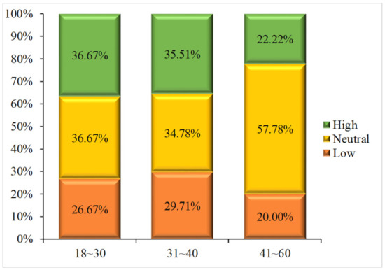
Figure 5.
The sensitivity of travelers of different ages to changes in expense-cost.
3.2.3. Analysis of the Sensitivity of Travelers with Different Occupations to Changes in Travel Cost
The sensitivity of travelers with different occupations to changes in travel cost is shown in Figure 6 and Figure 7. According to the survey results, among the respondents, students were the most sensitive to changes in expense-cost, while the staff of government and public institutions and enterprises were the most sensitive to the changes in time-cost between modes.
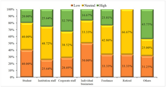
Figure 6.
The sensitivity of travelers with different occupations to changes in time-cost.
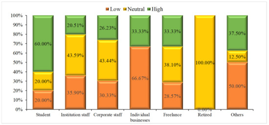
Figure 7.
The sensitivity of travelers with different occupations to changes in expense-cost.
3.2.4. Analysis of the Sensitivity of Travelers with Difference Incomes to Changes in Cost
The sensitivity of travelers of different incomes to a change in cost is shown in Figure 8 and Figure 9. According to the survey results, among the respondents, high-income travelers with a monthly income of more than 20,000 have the highest sensitivity to changes in time-cost, while their sensitivity to a change in expense-cost is the lowest.
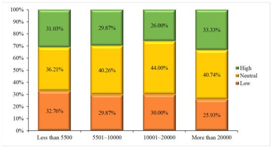
Figure 8.
The sensitivity of travelers with different incomes to a change in time-cost. (Note: RMB1000 ≈ USD140).
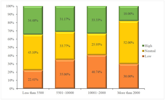
Figure 9.
The sensitivity of travelers with different incomes to a change in expense-cost. (Note: RMB1000 ≈ USD140).
3.3. Data Analysis
3.3.1. Reliability Test
The Cronbach’s alpha coefficient (α coefficient) was used to test the reliability of the questionnaire to determine whether the measurement items are highly consistent with the variables. It is generally believed that, when , the consistency and the reliability is high; when , the consistency and the reliability is acceptable; and when , the consistency and the reliability is low. The reliability test results showed that the Cronbach’s alpha coefficients of ATT, SN, PBC, BI, and SEN were 0.853, 0.895, 0.929, 0.908, and 0.691, respectively, indicating that the variables had good internal consistency.
3.3.2. Validity Test
We used the SPSS software to test the structural validity of the scale through exploratory factor analysis. SPSS is a combined software package. The basic functions of SPSS include data management, statistical analysis, chart analysis, output management and so on. It provides statistical analysis methods ranging from simple statistical description to complex multi-factor statistical analysis, such as exploratory analysis of data, statistical description, crosstab analysis, variance analysis, multiple regression, factor analysis, cluster analysis, nonlinear regression, logistic regression, etc. The results of the Kaiser–Meyer–Olkin (KMO) test and Bartlett’s spherical test of the scale showed that KMO = 0.845 (greater than 0.7), and the Bartlett’s spherical test value was significant (Sig. <0.001), indicating that there was a strong correlation between the observed variables, which were suitable for factor analysis.
The factor loading matrix was orthogonally rotated by the maximum variance method. After removing ATT1 and PBC6, whose factor loading values were less than 0.5, all factor loading values were greater than 0.5. The results are shown in Table 4, indicating that the scale had good structural validity.
Table 4.
Factor loading matrix after rotation.
3.3.3. Fitness Test
AMOS 4.0 was used for confirmatory factor analysis to test the fitness of the model. AMOS 4.0 is an independent product of SPSS Statistics software package and a powerful structural equation modeling tool. AMOS 4.0 shows the relationship between the assumed variables with an intuitive path diagram and offers more options for advanced SEM methods, enabling richer and more accurate synthesis than using factor or regression analysis alone. The results are shown in Table 5. It can be seen from the results in the table that all the fitness indexes of the model meet or basically meet the standards. In general, the model fits well, which indicates that the hypothesized theoretical model fits well with the actual data, as the model results are convincing.
Table 5.
Fitness test results.
4. Results and Discussion
4.1. Analysis of SEM Estimation Results
The estimated results of the standardized path coefficients among the potential variables are shown in Figure 10, and the path coefficients and significance are shown in Table 6.
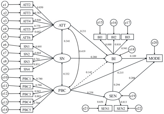
Figure 10.
Standardized path coefficient of SEM.
Table 6.
Load factor estimates and test values.
From Figure 10 and Table 6, it can be seen that ATT and SN have significant positive effects on BI. Among them, the path coefficient between ATT and BI is 0.211, showing a significant causal relationship (p = 0.004), and the path coefficient between SN and BI is 0.280, showing a significant causal relationship (p < 0.001). The path coefficient between PBC and BI is 0.159, but its influence does not reach the significance level (p = 0.057), indicating that there is no significant causal relationship between the two. The path coefficient between PBC and SEN is 0.258, and the significance level passes the test (p = 0.005), indicating that PBC has a significant positive impact on SEN. PBC and BI have significant positive effects on mode choice behavior, with a path coefficient and significance level of 0.215 (p = 0.003) and 0.189 (p = 0.014), respectively. In addition, SEN has significant positive effects on BI and mode choice behavior. The path coefficients are 0.258 (p < 0.001) and 0.208 (p = 0.013), respectively, indicating that the more sensitive travelers are to changes in cost, the stronger their intention to choose public transportation and the more inclined they are to choose public transportation. Among respondents, the sensitivity to change in expense-cost (SEN2) has a greater impact, indicating that the more sensitive travelers are to changes in expense-cost, the more inclined they are to choose public transportation.
4.2. Analysis of LCM Estimation Results
4.2.1. Selection of Explicit Variables
Individual travel mode choice behavior is affected by personal attributes, attitudes, subjective norms, perceived behavior control, sensitivity to changes in travel utility, and other factors. After several trials, we ultimately decided on individual gender (SEX), income (INCOME), attitude toward public transport punctuality (ATT4), the influence of the media and public opinion (SN2), public traffic waiting time (PBC2), and sensitivities to changes in time-cost and expense-cost (SEN1 and SEN2) as explicit variables. The results are shown in Table 7.
Table 7.
Explicit variables and corresponding level factors.
4.2.2. Parameter Estimation and Result Analysis
(1) Determining the Number of Latent Classes
This study uses the Mplus software to estimate the model parameters. The number of potential categories increases one by one. The best model, and the parameter estimation results, were obtained by comparing the results of a goodness-of-fit test. The fitness indexes of different LCM categories are shown in Table 8. The results showed that neither the χ2 test nor the G2 test rejected the hypothesis (p > 0.05), suggesting that a potential category model could be established. As the number of categories increases, the BIC index increases. The AIC index decreases first and then increases when the number of categories is five. As the sample size of this study is relatively small (N = 212), the AIC index is taken as the main standard, with four categories in the final selection model.
Table 8.
The fitness test results of the latent class model (LCM).
(2) Parameter Estimation and Reliability Test
The travelers in the sample were divided into four latent classes through a goodness-of-fit test, and the maximum likelihood method was adopted for parameter estimation. The results are shown in Table 9.
Table 9.
The parameter estimation results of the LCM.
In order to illustrate the credibility of the classification results of the model, the attribution probability matrix for the determined categories is calculated, and the results are shown in Table 10. It can be seen that the travelers of each category have a high probability of belonging to each potential category—respectively, 0.934, 0.946, 0.886, and 0.976, and the misjudgment rate among all the categories is very low, indicating that the classification effect is good.
Table 10.
The latent class probability matrix table.
(3) Potential Category Naming and Policy Suggestions
Through a cross analysis of explicit variables and categories, the characteristics of various travelers are summarized. The analysis results are shown in Figure 11, Figure 12, Figure 13, Figure 14, Figure 15, Figure 16 and Figure 17. The OX axes of these figures represent four latent classes of respondents. The OY axes of these figures are the proportion of respondents in each class for different observed variables. The legends of Figure 11 and Figure 12 are the observed variables of sex and monthly income. The legends of Figure 13, Figure 14 and Figure 15 are respondents’ answers to ATT4, SN2, and PBC2. The options in the scale are “strongly disagree”, “disagree”, “general”, “agree”, and “strongly agree”, with values ranging from 1 to 5. The legends of Figure 16 and Figure 17 are respondents’ sensitivity to the changes in time-cost and expense-cost respectively, that is, high sensitivity to a change in cost, neutral sensitivity to a change in cost, and low sensitivity to a change in cost.
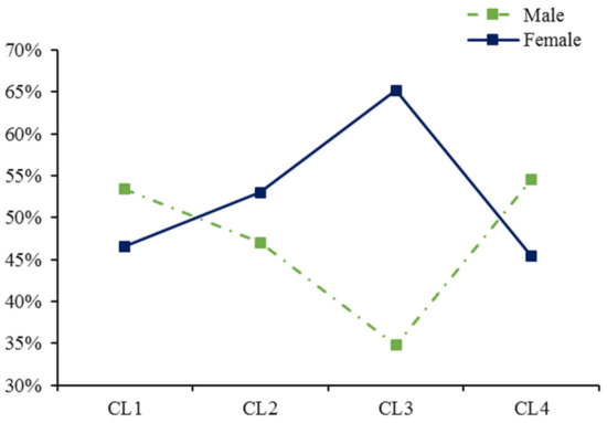
Figure 11.
Gender—latent classification characteristic.
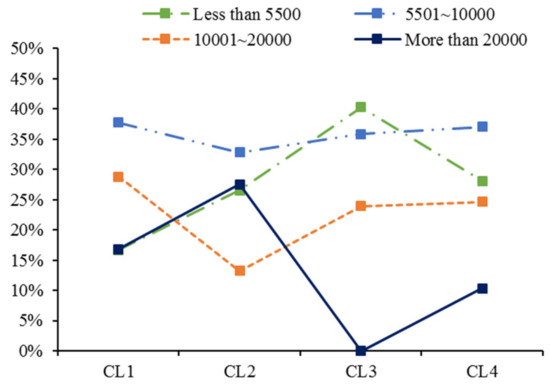
Figure 12.
Income—latent classification characteristic. (Note: RMB1000 ≈ USD140).
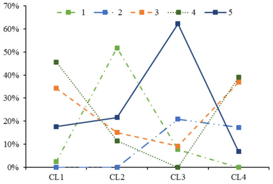
Figure 13.
Attitude toward public transport—latent classification characteristic.
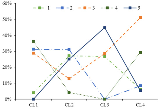
Figure 14.
The influence of media and public opinion—latent classification characteristic.
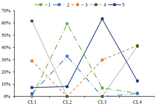
Figure 15.
The feeling of waiting for public transportation—latent classification characteristic.
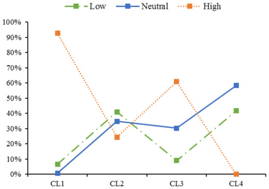
Figure 16.
Sensitivity to changes in time-cost—latent classification characteristic.
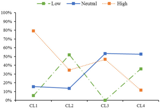
Figure 17.
Sensitivity to changes in expense-cost—latent classification characteristic.
It can be seen from Figure 11 that, in the CL3 category, the proportion of female travelers is relatively high, while in the other three categories, the proportion of male travelers and female travelers is similar, which is close to the gender distribution of the survey samples.
According to Figure 12, low-income travelers account for a higher proportion in the CL3 category, while high-income travelers account for a higher proportion in the CL1, CL2, and CL4 categories.
As can be seen from Figure 13, the CL2 category has the lowest positive evaluation on public transport punctuality; 51.8% of travelers strongly disagree that choosing public transport is more punctual. The CL3 category has the highest positive evaluation of public transport punctuality, as the proportion of travelers who strongly agree that choosing public transport is more punctual reaches 62.2%. The CL1 and CL4 categories are similar; their evaluations of public transport punctuality are neutral and positive.
As can be seen from Figure 14, the influence of media and public opinion on CL3 travelers is polarized. Here, 44.7% of CL3 categories have a score of 5, while 26.7% have a score of 1. The rest are neutral. Among the CL2 travelers, 25% of the travelers scored 5, 27.1% of the travelers scored 1, and 30.9% of the travelers scored 2. The overall evaluation was low, suggesting that the CL2 category was not easily affected by media and social public opinion. CL1 mainly focuses on scoring 2, 3, and 4, which are evenly distributed. Similar to CL1, CL4 mainly focuses on scoring 3 and 4, which are mostly neutral.
Figure 15 shows that CL2 travelers have the lowest evaluation of public transport waiting time, while CL3 travelers have the highest positive evaluation of public transport waiting time. CL1 and CL4 travelers’ evaluations of the public transport waiting time are mostly neutral and positive.
From Figure 16, it can be seen that CL1 travelers have the highest sensitivity to changes in time-cost—that is, the change in time-cost that can facilitate a mode transfer is smallest for this type of traveler. CL3 travelers have high sensitivity, while CL2 and CL4 travelers have low–neutral sensitivity.
As can be seen from Figure 17, CL1 travelers have the highest sensitivity to changes in expense-cost—that is, the change in expense-cost that can facilitate mode transfer is lowest for this type of traveler. CL3 travelers have high sensitivity, CL4 travelers have low–neutral sensitivity, and CL2 travelers have the lowest sensitivity.
To sum up, the naming and policy suggestions for different types of travelers are as follows:
CL1: Rational decision making. This kind of travelers’ evaluations of public transportation punctuality and waiting time are neutral and positive. The travelers have no extreme feelings about the media and public opinion. However, their sensitivities to changes in time-cost and expense-cost are the highest. This type of traveler should be the main target for priority development strategies for public transport and economic leveraging. Reducing the travel time-cost of public transportation (for example, improving the service frequency of public transportation or setting up bus lanes) or increasing the expense-cost of private transportation (for example, raising parking fees in downtown areas or imposing congestion pricing) can attract such travelers to use public transportation.
CL2: Focus on feeling. These kinds of travelers have high incomes, low evaluations of public transportation punctuality and waiting time, and are not easily influenced by media and public opinion. They are also not sensitive to changes in the time-cost and expense-cost. It is speculated that such travelers prefer private transportation. Therefore, this group of people is the main target of restrictive development strategies and travel prohibition strategies. Such travelers who use private transportation will be transferred to public transportation through measures such as traffic restrictions.
CL3: Sensitive to cost. Female travelers in this category account for a relatively high proportion, and their income levels are lower than those in other categories. They are sensitive to changes in time-cost and expense-cost and have the highest positive evaluation of the punctuality and waiting time of public transportation. The influence of media and public opinion on these travelers is polarized. CL3 travelers have the highest positive evaluation of public transport and are very sensitive to changes in cost. Therefore, travelers of this type who often use public transport can be stabilized by priority development strategies for public transport, such as establishing bus lanes or increasing the preferential treatment for public transport. In addition, private traffic users among such travelers could be encouraged to transfer to public transportation by increasing parking fees in central areas or increasing enforcement of parking violations.
CL4: Bounded rational decision making. The income level of such travelers is above average. These travelers are not sensitive to changes in time-cost and expense-cost. Their evaluation of the punctuality and waiting time of public transportation is neutral. The influence of media and public opinion on them is not obvious. It is speculated that the mode choice behavior of such travelers is relatively random. Therefore, these types of travelers could be encouraged to use public transit by restraining private traffic and prioritizing the development of public transport, such as improving the convenience and comfort of public transport, strengthening the publicity of public transport to encourage bus travel, and implementing car restrictions.
5. Conclusions
In this paper, “sensitivity to the change in travel utility” is considered a psychological factor that influences travel behavior. Based on the data of the travel behavior survey, a SEM considering indifference threshold was established, and the influencing factors behind travelers’ choices between private transportation and public transportation were analyzed. The analysis results show that: (1) Travelers’ sensitivities to changes in travel utility have a great impact on mode choice intention and mode choice behavior. (2) The influence of subjective norms on mode choice intention is secondary to a traveler’s sensitivity to the utility difference between modes. (3) The influence of attitude on mode choice intention is secondary to subjective norms. (4) Perceptual behavior control has the strongest influence on travel choice behavior.
In addition, in order to further explore the heterogeneity of a traveler’s mode choice behavior, travelers were subdivided into different types by establishing an LCM considering the indifference threshold. Finally, different traffic management policies are proposed for different types of travelers. The results show that: (1) Rational decision-making travelers should be the main object of priority development strategies for public transport and economic leveraging. (2) The travelers focused on feeling should be the main targets of restrictive development strategies and travel prohibition strategies. (3) For cost-sensitive travelers who often use public transportation, a priority development strategy of public transportation can be adopted to stabilize this type of transportation, and a restrictive development strategy can be adopted to guide the private traffic users among such travelers to switch to public transportation. (4) Travelers with limited rational decision-making can be guided in two ways: By controlling private transportation and by giving priority to the development of public transport.
This paper investigates travel mode choice by the sensitivity of the travellers. However, there are still some limitations. For example, the TPB assumes that behavior is the result of a linear decision-making process, and does not consider that it can change over time. Future research can focus on the dynamic evolution of travelers’ mode choice behavior over time. At the same time, the influence of other factors and various combinations of factors can be studied.
Author Contributions
X.Z. and H.Z. collected the data; X.Z. built the model, performed the analyses and validation, and prepared the manuscript; X.Z. and H.G. formulated the overarching research goals and aims; H.G. supervised and obtained the grant for the study; X.Z., H.G. and J.Z. restructured and edited the manuscript.
Funding
This research was funded by the National Natural Science Foundation of China, grant numbers 71971005.
Acknowledgments
The authors are very grateful to all the participants who filled in the questionnaire. We sincerely thank the reviewers for their professional suggestions and the editors for their patient and meticulous work.
Conflicts of Interest
The authors declare no conflict of interest.
References
- Xv, J.Q. Fundamentals of Traffic Engineering; China Communications Press: Beijing, China, 2015. [Google Scholar]
- Simon, H.S. A behavioral model of rational choice. Q. J. Econ. 1955, 1, 99–118. [Google Scholar] [CrossRef]
- Krishnan, K.S. Incorporating thresholds of indifference in probabilistic choice models. Manag. Sci. 1977, 23, 1224–1233. [Google Scholar] [CrossRef]
- Lioukas, S.K. Thresholds and transitivity in stochastic consumer choice a multinomial logit analysis. Manag. Sci. 1984, 30, 110–122. [Google Scholar] [CrossRef]
- Mahmassani, H.S.; Chang, G.L. On boundedly rational user equilibrium in transportation systems. Transp. Sci. 1987, 21, 89–99. [Google Scholar] [CrossRef]
- Mahmassani, H.S.; Chang, G.L. Experiments with departure time choice dynamics of urban commuters. Transp. Res. Pt. B-Methodol. 1986, 20, 297–320. [Google Scholar] [CrossRef]
- Mahmassani, H.S.; Jou, R.C. Transferring insights into commuter behavior dynamics from laboratory experiments to field surveys. Transp. Res. Pt. A-Policy Pract. 2000, 34, 243–260. [Google Scholar] [CrossRef]
- Di, X.; Liu, H.X.; Zhu, S.; David, M.L. Indifference bands for boundedly rational route switching. Transportation 2017, 44, 1169–1194. [Google Scholar] [CrossRef]
- Carrion, C.; Levinson, D.M. Route choice dynamics after a link restoration. Transp. B-Transp. Dyn. 2019, 7, 1155–1174. [Google Scholar] [CrossRef]
- Li, T.; Guan, H.Z.; Liang, K.K. Day-to-Day dynamical evolution of network traffic flow under bounded rational view. Acta Phys. Sin. 2016, 65, 17–27. [Google Scholar]
- Zhang, X.J.; Guan, H.Z.; Zhao, L.; Bian, F. Nested Logit Model on Travel Mode Choice under Boundebly Rational View. J. Transp. Syst. Eng. Inf. Technol. 2018, 6, 110–116. [Google Scholar]
- Wei, W.; Hui, J.S.; Zhi, W.W.; Wu, J.J. Optimal transit fare in a bimodal network under demand uncertainty and bounded rationality. J. Adv. Transp. 2014, 48, 957–973. [Google Scholar] [CrossRef]
- Guilford, J.P. Psychometric Methods; McGraw-Hill: New York, NY, USA, 1954. [Google Scholar]
- Quandt, R.E. A probabilistic theory of consumer behavior. Q. J. Econ. 1956, 70, 507–536. [Google Scholar] [CrossRef]
- Georgescu-Roegen, N. Threshold in Choice and the Theory of Demand. Econom. J. Econ. Soc. 1958, 157–168. [Google Scholar] [CrossRef]
- Han, Y.; Li, W.Y.; Wei, S.S.; Zhang, T.T. Research on Passenger’s Travel Mode Choice Behavior Waiting at Bus Station Based on SEM-Logit Integration Model. Sustainability 2018, 10, 1996. [Google Scholar] [CrossRef]
- Si, Y.; Guan, H.Z.; Cui, Y.C. Research on the Choice Behavior of Taxis and Express Services Based on the SEM-Logit Model. Sustainability 2019, 11, 2974. [Google Scholar] [CrossRef]
- Zhu, H.Y.; Guan, H.Z.; Han, Y.; Li, W.Y. A Study of Tourists’ Holiday Rush-Hour Avoidance Travel Behavior Considering Psychographic Segmentation. Sustainability 2019, 11, 3755. [Google Scholar] [CrossRef]
- Terry, L.; Cathy, H.C.H. Predicting behavioral intention of choosing a travel destination. Tour. Manag. 2006, 27, 589–599. [Google Scholar]
- Christian, A.K.; Anke, B. A comprehensive action determination model: Toward a broader understanding of ecological behaviour using the example of travel mode choice. J. Environ. Psychol. 2010, 30, 574–586. [Google Scholar]
- Zhang, L.; Ren, G.; Wang, W.J. Unsafe Behavior Improved Model for Bicycle Riding Based on Theory of Planned Behavior. China. Saf. Sci. J. 2010, 20, 43–48. [Google Scholar]
- Chen, J.; Yan, Q.P.; Yang, F. SEM-Logit Integration Model of Travel Mode Choice Behaviors. J. South China. Univ. Tech. 2013, 41, 51–57. [Google Scholar]
- Jing, P.; Juan, Z.C. Analysis of intercity travel mode choice in the theory of planned behavior. China. Sciencepaper. 2013, 8, 1088–1094. [Google Scholar]
- Szabolcs, D.; Sarbast, M. Sustainable Urban Transport Development with Stakeholder Participation, an AHP-Kendall Model: A Case Study for Mersin. Sustainability 2018, 10, 3647. [Google Scholar]
- Omid, G.; Sarbast, M.; Thomas, B.; Szabolcs, D. Sustainable Urban Transport Planning Considering Different Stakeholder Groups by an Interval-AHP Decision Support Model. Sustainability 2019, 11, 9. [Google Scholar]
- William, H.G.; David, A.H. A latent class model for discrete choice analysis: Contrasts with mixed logit. Transp. Res. Pt. B-Methodol. 2003, 37, 681–698. [Google Scholar]
- Wen, C.H.; Wang, W.C.; Fu, C. Latent class nested logit model for analyzing high-speed rail access mode choice. Transp. Res. Pt. E-Logist. Transp. Rev. 2012, 48, 545–554. [Google Scholar] [CrossRef]
- Molin, E.; Mokhtarian, P.; Kroesen, M. Multimodal travel groups and attitudes: A latent class cluster analysis of Dutch travelers. Transp. Res. Part A Policy Pract. 2016, 83, 14–29. [Google Scholar] [CrossRef]
- López-Bonilla, L.M.; López-Bonilla, J.M. Postmodernism and Heterogeneity of Leisure Tourist Behavior Patterns. Leis. Sci. 2009, 31, 68–83. [Google Scholar] [CrossRef]
- William, G.; Mark, N.H.; Bruce, H.; Pushkar, M. A latent class model for obesity. Econ. Lett. 2014, 123, 1–5. [Google Scholar]
- Wen, C.H.; Lai, S.C. Latent class models of international air carrier choice. Transp. Res. Pt. E-Logist. Transp. Rev. 2010, 46, 211–221. [Google Scholar] [CrossRef]
- Ajzen, I. The Theory of Planned Behavior. Org. Behav. Hum. Decis. Process. 1991, 50, 179–211. [Google Scholar] [CrossRef]
- Arellana, J.; Daly, A.; Hess, S.; de Dios Ortúzar, J.; Rizzi, L.I. Development of Surveys for Study of Departure Time Choice: Two-Stage Approach to Efficient Design. Transp. Res. Rec. J. Res. Board. 2012, 2303, 9–18. [Google Scholar] [CrossRef]
- Thorhauge, M.; Haustein, S.; Cherchi, E. Accounting for the Theory of Planned Behaviour in departure time choice. Transp. Res. Pt. F: Trac. Psychol. Behav. 2016, 38, 94–105. [Google Scholar] [CrossRef]
© 2019 by the authors. Licensee MDPI, Basel, Switzerland. This article is an open access article distributed under the terms and conditions of the Creative Commons Attribution (CC BY) license (http://creativecommons.org/licenses/by/4.0/).