Article

An Enhanced MOPSO Algorithm for Energy-Efficient Single-Machine Production Scheduling

School of Economics & Management, Xiamen University of Technology, Xiamen 361024, China
*
Author to whom correspondence should be addressed.
Sustainability 2019, 11(19), 5381; https://doi.org/10.3390/su11195381
Submission received: 2 August 2019 / Revised: 19 September 2019 / Accepted: 23 September 2019 / Published: 28 September 2019

Abstract

:
In recent years, the concerns on energy efficiency in manufacturing systems have been growing rapidly due to the pursuit of sustainable development. Production scheduling plays a vital role in saving energy and promoting profitability for the manufacturing industry. In this paper, we are concerned with a just-in-time (JIT) single machine scheduling problem which considers the deterioration effect and the energy consumption of job processing operations. The aim is to determine an optimal sequence for processing jobs under the objective of minimizing the total earliness/tardiness cost and the total energy consumption. Since the problem is NP -hard, an improved multi-objective particle swarm optimization algorithm enhanced by a local search strategy (MOPSO-LS) is proposed. We draw on the idea of k-opt neighborhoods and modify the neighborhood operations adaptively for the production scheduling problem. We consider two types of k-opt operations and implement the one without overlap in our local search. Three different values of k have been tested. We compare the performance of MOPSO-LS and MOPSO (excluding the local search function completely). Besides, we also compare MOPSO-LS with the well-known multi-objective optimization algorithm NSGA-II. The experimental results have verified the effectiveness of the proposed algorithm. The work of this paper will shed some light on the fast-growing research related to sustainable production scheduling.

1. Introduction

The manufacturing industry has been regarded as an intensive energy consumer. To achieve sustainable development goals, a number of regulations are urging the manufacturers to adopt energy-saving measures. In addition to an upgrade of production equipment, which is usually costly, the possibility of using soft techniques to achieve energy savings should be emphasized. In fact, production scheduling could play a significant role in reducing the energy consumption of manufacturing processes. However, the traditional production scheduling software, which is often embedded in the company’s ERP or MES, has been designed solely for the productivity or profitability goal, without consideration of sustainability impacts. To take energy consumption and other environmental factors into consideration, the scheduling models and algorithms need to be significantly revised or even rewritten. In the redevelopment process, a major difficulty is that the energy model, which characterizes the power consumption of manufacturing activities, is highly industry-dependent and factory-dependent, and therefore, energy-efficient production scheduling algorithms are not universally applicable and have to be designed specifically for each company. Currently, some energy-intensive manufacturers (like steel companies) have adopted energy-saving production scheduling techniques, and the procedure is waiting to be extended and applied to other industries. Another issue that prevents the application of such scheduling technologies is the high computational complexity. The simultaneous consideration of energy-related aspects will complicate the scheduling model (leading to more constraints and variables), which requires more powerful optimization algorithms to solve. This poses a theoretical challenge to the operations research and management science community.
Energy-efficient production scheduling problems have been extensively studied by a number of researchers in recent years [1,2,3,4]. In the existing research, considerations for energy efficiency can be divided into two categories, i.e., energy-related objectives and energy-related constraints. Wang et al. [1] study a bi-objective single machine batch scheduling problem with non-identical job sizes. Zhang and Chiong [5] propose an enhanced multi-objective genetic algorithm to solve the job shop scheduling problem minimizing total energy consumption and total weighted tardiness. Wu et al. [6] investigate the flexible job-shop scheduling problem with the objective of minimizing total energy consumption and makespan. They consider the deterioration effect as well. Liao et al. [7] use MOPSO to address the bi-objective single machine scheduling problem with energy consumption constraints. Módos et al. [8] consider a production scheduling problem with large electricity consumption. The energy-related constraint requires that, in the specified time intervals, the total energy consumption should not exceed a given limit.
Just-in-time (JIT) objectives are commonly considered in production scheduling problems. Under the JIT logic, both earliness and tardiness (with respect to due dates) should be penalized [9,10]. The former can cause inventory holding costs such as storage cost and extra delivering cost (especially for perishable goods), while the latter can cause loss of reputation, sale and may even cause penalty.
In real-world manufacturing systems, the processing times of certain jobs can be longer than their nominal values because of the deterioration effect (deterioration effect refers to the phenomenon that a job requires longer processing time if its starting time is postponed or later than expected). There are varieties of factors that may cause deterioration such as high workload of machines, insertion of maintenance activities, and fatigue of human operators [11,12]. Deterioration can also be explained by industry-specific reasons, for example, a steel slab in the hot rolling production process has to be reheated (which takes extra processing time) if it has been kept waiting for a long time which brings a significant decline in temperature [13].
To the best of our knowledge, there are no results in the existing literature for production scheduling problems that integrate the JIT objective, the energy-saving requirement and explicit consideration of the deterioration effect. Production systems with the above characteristics are commonly observed in mechanical and metal manufacturing companies. Note that the single-machine JIT scheduling problem with a deterioration effect is NP -hard [14], which means the time required by an exact algorithm to solve the problem increases exponentially with the number of jobs. Hence, a multi-objective particle swarm optimization algorithm enhanced by local search (MOPSO-LS) is presented in this paper to obtain near-optimal solutions for the discussed problem.
The rest of this paper is organized as follows. Section 2 introduces the basic definitions and notations for the bi-objective single-machine scheduling problem with deterioration. Section 3 describes the proposed MOPSO-LS algorithm. Computational results are shown in Section 4. Conclusions and future work are presented in Section 5.

2. The Scheduling Problem

2.1. Problem Statement

The problem is described as follows. A set of jobs labeled as J = { j | j = 1 , 2 , , n } are to be scheduled on a single machine. The aim is to obtain the best sequence for processing the set of jobs to minimize the total weighted earliness/tardiness ( T W E T ) and the total energy consumption ( T E C ). Each job j is characterized by a basic processing time t b p j , a latest starting time t l s j , a weight w j and a due date d j . For a given sequence of jobs, the completion time t c j of job j can be determined, and the earliness/tardiness of job j is defined as e t j = t c j d j . One objective is to minimize the total weighed earliness/tardiness T W E T = j = 1 n w j e t j . Another objective is to minimize the total energy consumption T E C = j = 1 n t p j e j , where e j is the power consumption for processing job j per unit time and t p j is the actual processing time of job j.
With the deterioration effect in consideration, the actual processing time of each job j is variable and determined by the basic processing time t b p j and the starting time t s j . For each job j, when the starting time t s j is earlier than or equal to its latest starting time t l s j , the actual processing time t p j is equal to its basic processing time t b p j . Otherwise, the increment in actual processing time t p j is proportional to the delay of starting time, i.e., t s j t l s j . Therefore, t p j can be calculated as follows:
t p j = t b p j + b j max { 0 , t s j t l s j } ,
where b j is the deterioration coefficient of job j.
The other assumptions for the problem are stated as follows (these are standard assumptions for the modeling of scheduling problems and are normally satisfied in practical situations):
  • All jobs are available at time zero.
  • The machine can handle only one job at a time.
  • There are no precedence relations between the jobs.
  • Preemption is not allowed.
  • Setup times are not considered.

2.2. A Small Example

Consider a set of eight jobs labeled as j { 1 , 2 , 3 , 4 , 5 , 6 , 7 , 8 } . The information about each job is shown in Table 1. Obviously, each possible sequence of the jobs corresponds to a feasible solution, so the number of feasible solutions for this instance is: 8 ! = 40 , 320 . Figure 1 shows the objective space of this instance and marks all the non-dominated solutions. In this case, there are eight non-dominated solutions in total, which constitute the Pareto front, i.e., the set of Pareto-optimal solutions (we say a solution is Pareto-optimal if neither objective can be improved without sacrificing the other objective).

3. The Proposed Algorithm

3.1. The Basic PSO Algorithm

The proposed algorithm adopts MOPSO as the main framework and incorporates an enhanced local search method to promote efficiency. We first make a brief introduction to the basic principles of PSO. The PSO algorithm is a population-based stochastic optimization technique inspired by the social behavior of bird flocking or fish schooling. It is a well-known meta-heuristic algorithm for solving both continuous and combinatorial optimization problems.
Firstly, the algorithm generates a population of particles and the position of each particle represents a potential solution in the search space for the considered problem. According to the evaluation of the objective function to be optimized, each particle has a fitness value. Then, the fitness determines the flying direction and speed of the particles. In each iteration, two types of best positions are preserved. One is called the personal best position ( p best ) which represents the best solution that each particle has achieved so far. The other is called the global best position ( g best ) which represents the best position obtained so far by all the particles. Finally, the particles learn from these two best positions based on their current flying routes, and the positions of the particles get updated in each iteration. The iterations continue until the convergence criterion is satisfied.

3.2. Encoding and Decoding

We use the largest position value (LPV) rule as the decoding method, which transforms continuously encoded particles into discrete solutions. Simply speaking, the decoded solution records the relative order of the corresponding position values (from largest to smallest). For example, for a particle p t = ( 2.38 , 0.55 , 3.64 , 3.98 , 1.68 , 1.26 , 0.8 , 2.33 ) , its corresponding job sequence is S p t = ( 2 , 5 , 8 , 1 , 3 , 6 , 4 , 7 ) , because the fourth value in p t is the largest (rank 1) and the third value in p t is the smallest (rank 8).

3.3. Solution Initialization

Generally, the initial population is generated by specific heuristic rules combined with some random methods to get high-quality and distinct solutions. However, to encourage solution diversity and to facilitate the evaluation of the k-opt neighborhood operations, the individuals of the initial population are completely randomized in our proposed algorithm.

3.4. Sorting of Solutions

In multi-objective optimization settings, Pareto dominance is the main criterion for distinguishing the quality of different solutions. For our research, both objectives aim at finding the minimum. In this case, solution x 1 with objective values ( T W E T 1 , T E C 1 ) is said to dominate solution x 2 with objective values ( T W E T 2 , T E C 2 ) if either one of the following two conditions is satisfied:
  • T W E T 1 < T W E T 2 and T E C 1 T E C 2
  • T W E T 1 T W E T 2 and T E C 1 < T E C 2
The relation will be denoted by x 1 x 2 . Two solutions are treated equally in the same Pareto rank if they are mutually non-dominated. All the non-dominated solutions are stored in an external archive.
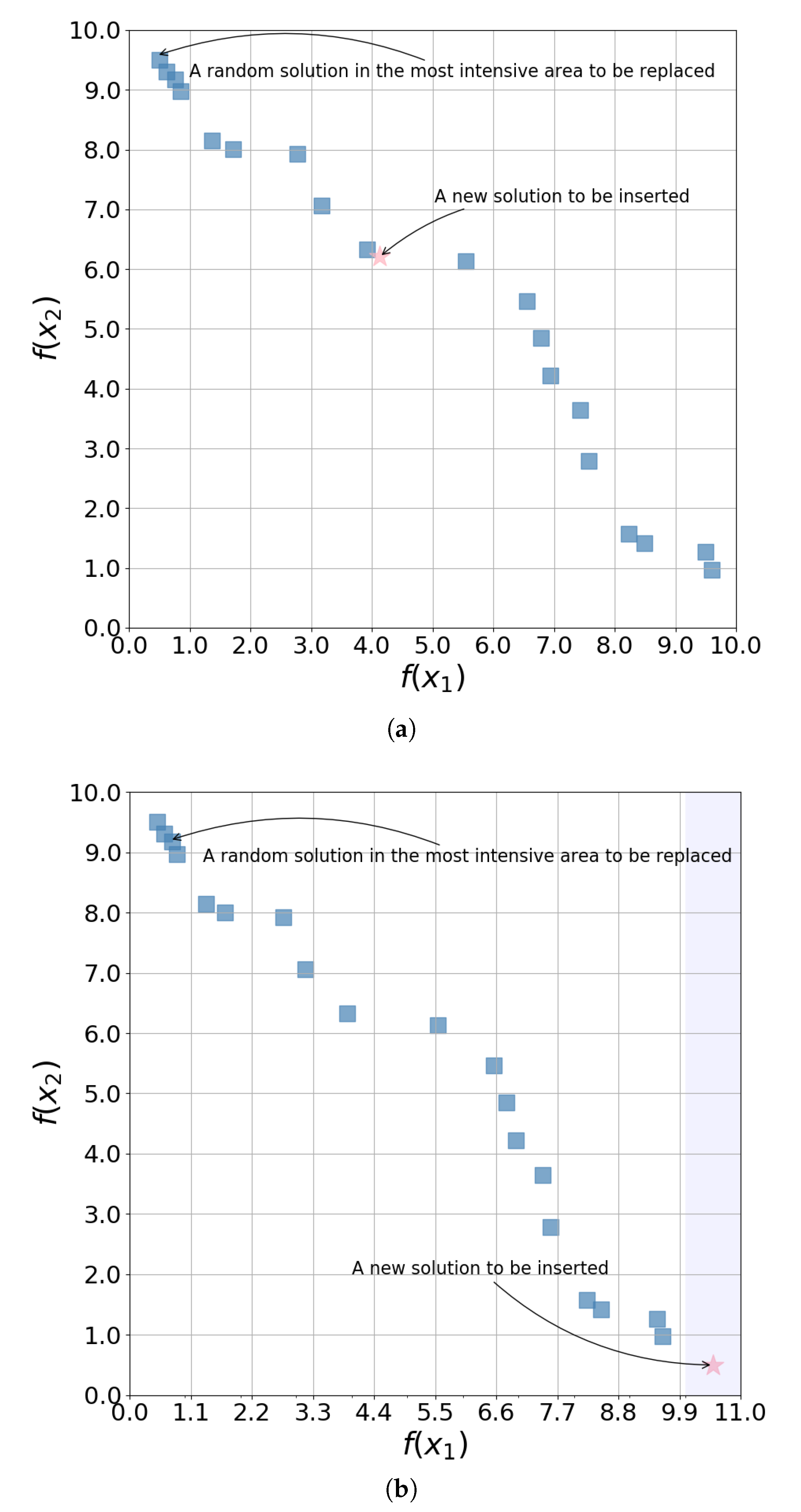
In addition to Pareto dominance, the adaptive grid method proposed by Coello Coello [15] is used to sort solutions that are not mutually dominated. The aim is to avoid over-crowded solutions and obtain evenly distributed non-dominated solutions for the decision maker. Figure 2 shows the insertion of a new solution in the adaptive grid with grid size n d = 10 .

3.5. External Repository and Updating Mechanisms

In standard PSO intended for single-objective optimization, either the personal best solution associated with each particle or the global best solution is an individual solution. However, it is necessary to preserve a number of equally optimal (non-dominated) solutions when addressing multi-objective optimization problems. For this purpose, we build an external repository (denoted by a set ϕ ) to save all the historical non-dominated solutions found in the search process.
The maintenance rules are described as follows. In each iteration, if the newly produced solutions are all dominated by some existing solutions in ϕ , nothing happens. If there are any new non-dominated solutions, then insert all of them into the repository and the dominated solutions originally in the repository are eliminated.

3.6. The Mutation Operator

We apply a mutation operator to enhance the global searching capability of MOPSO (the concept of mutation is adapted from genetic algorithm, representing a perturbation technique which alters the current solutions slightly in the hope of finding better solutions). The mutation operator is applied to the particles of the swarm after the position updating process. Specifically, we use a mutation index (represented as m u t I n d e x ) to control the probability of mutation. When m u t I n d e x is a positive real number, the mutation operator will be applied to each particle with a probability of m u t I n d e x . In the selected particle, the mutation operator changes the value of a randomly identified position to a real number generated from the uniform distribution whose interval is centered at its original value with m u t R a d i u s as its radius. The m u t I n d e x and m u t R a d i u s mentioned above can be calculated as follows:
m u t I n d e x = 1 i t e r i t e r M a x × p m 3 2
m u t R a d i u s = r a n g e M a x × m u t I n d e x 2 ,
where i t e r and i t e r M a x represents the current iteration number and the maximum iteration number of MOPSO, p m is the mutation rate defined in MOPSO, and r a n g e M a x is set at 4 in our algorithm.

3.7. Local Search

The two-opt neighborhood operator, which reverses one segment of the sequence, is the most commonly used operator to generate neighboring solutions for routing problems. The idea can be extended to k 1 segments (k-opt). However, the operator needs to be modified in our research since a scheduling problem is different from a routing problem.
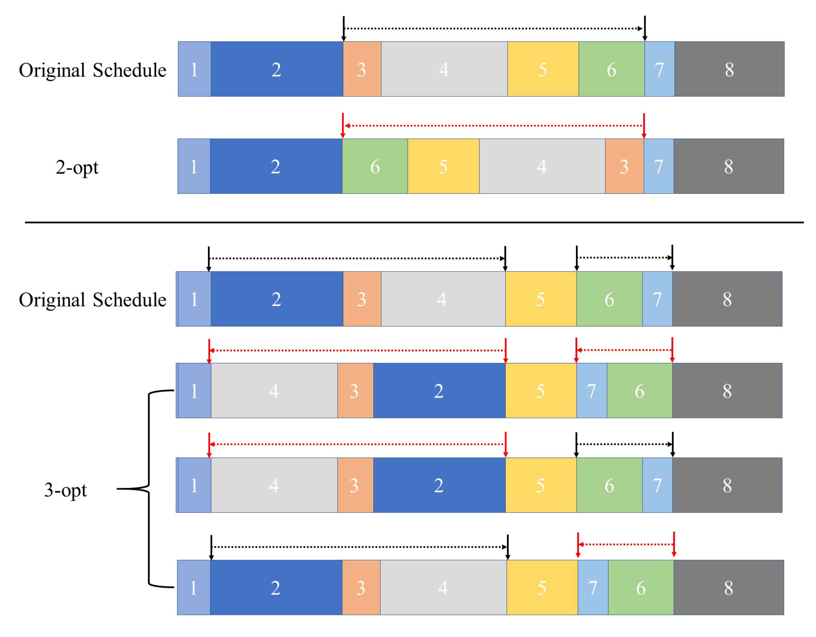
We define the k-opt neighborhood operations as follows. For a given sequence, we select k 1 segments randomly, and then we reverse some of these segments. Since each of the segments may or may not be reversed, there are a number of possible combinations. If the number of selected segments is k 1 , there are i = 1 k 1 C k 1 i ways to rearrange a schedule. For example, when considering 2 segments (3-opt), there are three possible outcome solutions (Figure 3). Similarly, for the case of three segments (four-opt), there are seven possible outcome solutions.
It is supposed that the selected segments do not have any overlap, because in the case of overlap, the order of reversing the segments will affect the final solutions. For example, consider two segments with an overlap (shown in Figure 4). For the original sequence S 0 = ( 1 , 2 , 3 , 4 , 5 , 6 , 7 , 8 ) , the first segment is from the second job to the sixth job and the second segment is from the fifth job to the seventh job. If we reverse the first segment first, we get the sequence S 1 = ( 1 , 6 , 5 , 4 , 3 , 2 , 7 , 8 ) , and then we reverse the second segment which is currently filled with jobs ( 3 , 2 , 7 ) . However, if we reverse the second segment first, we get the sequence S 2 = ( 1 , 2 , 3 , 4 , 7 , 6 , 5 , 8 ) , and then we reverse the first segment which is currently filled with jobs ( 2 , 3 , 4 , 7 , 6 ) . The resulting solutions will certainly be different in these two cases. To avoid confusion, we assume the selected segments for k-opt operations are overlap-free.
After the solution set ϕ in external repository has been updated in each iteration, the k-opt operator is performed on one of the solutions in ϕ . All solutions have equal probabilities of being selected. The new solutions produced by this operation will be added to ϕ . Then all the solutions will be evaluated and saved according to the updating mechanisms introduced before.

3.8. MOPSO-LS Framework

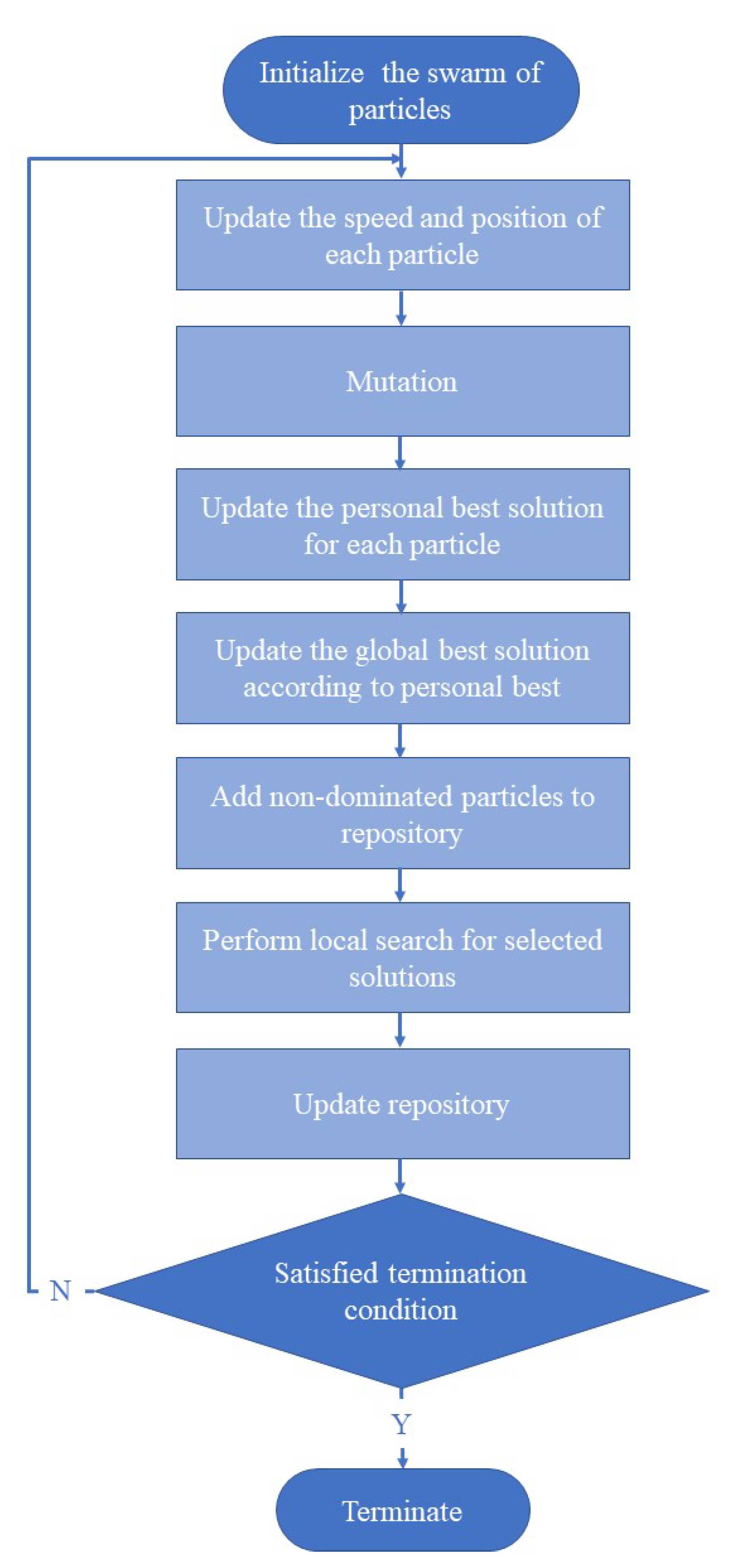
The entire algorithm structure of the MOPSO-LS is shown in Figure 5. Compared with the standard PSO workflow, our algorithm features a novel mutation operator and local search module, which greatly enhances the exploitation ability for coping with large-scale search space. In addition, the mechanisms for handling multi-objective optimization are also important contributors to the overall algorithm but not directly reflected in the flowchart.

4. Computational Experiments

4.1. Experimental Settings

Because there is no standard data set for the studied problem, we followed the data generation rules in literature for scheduling problems with deteriorating jobs and scheduling problems with energy consumption considerations. The parameters generated for the studied scheduling problem are described as follows and summarized in Table 2.
  • The basic processing time t b p j of each job is generated uniformly from u n i f ( 1 , 100 ) .
  • The deterioration factor of each job b j is generated from the uniform distribution u n i f ( 0 , 1 ) .
  • The latest starting time of each job t l s j = 30 × n × u n i f ( 0 , 1 ) where n is the number of jobs.
The true Pareto front of each instance was not known, but for comparison purpose, we generated an approximate Pareto front for each instance by the following steps. First, all algorithms including MOPSO-LS (2-opt), MOPSO-LS (3-opt), MOPSO-LS (4-opt), MOPSO (excluding local search) and NSGA-II were repeated 20 times. Then, we identified all the non-dominated solutions from the solutions found by the above algorithms and these non-dominated solutions constitute the approximate Pareto front.

4.2. The Performance Measures

Convergence to the Pareto front and evenness of solution distribution were two main criteria for assessing multi-objective optimization algorithms. In accordance with these requirements, we adopt the generational distance (GD) measure [16] and the spacing (SP) measure [17] to evaluate the performance of algorithms.
GD measures the distance between the set of non-dominated solutions found by the algorithm and the (approximate) Pareto front [16]. GD is defined as follows:
G D = i = 1 m d i 2 m ,
where m is the number of non-dominated solutions found and d i is the Euclidean distance between solution i and its nearest counterpart solution from the Pareto front.
SP measures the spread (distribution evenness) of the solutions found [17]. SP is defined as follows:
S P = 1 m 1 i = 1 m ( d ¯ d i ˜ ) 2 ,
where d ¯ = i = 1 m d i ˜ / m and d i ˜ is the Manhattan distance between solution i and its nearest neighbor solution in the set of non-dominated solutions found, formally defined as follows:
d i ˜ = min j , j i { | f 1 ( x i ) f 1 ( x j ) | + | f 2 ( x i ) f 2 ( x j ) | } .

4.3. Parameter Tuning Experiments

The setting of parameters can have a vital impact on the performance of algorithms. In the proposed MOPSO-LS, the weight ω , learning factors c 1 , c 2 , mutation probability p m , maximum velocity V max and the grid size n d [15] are important parameters. To find the best settings, we applied a design of experiments (DOE) approach to study the influence of these six parameters.
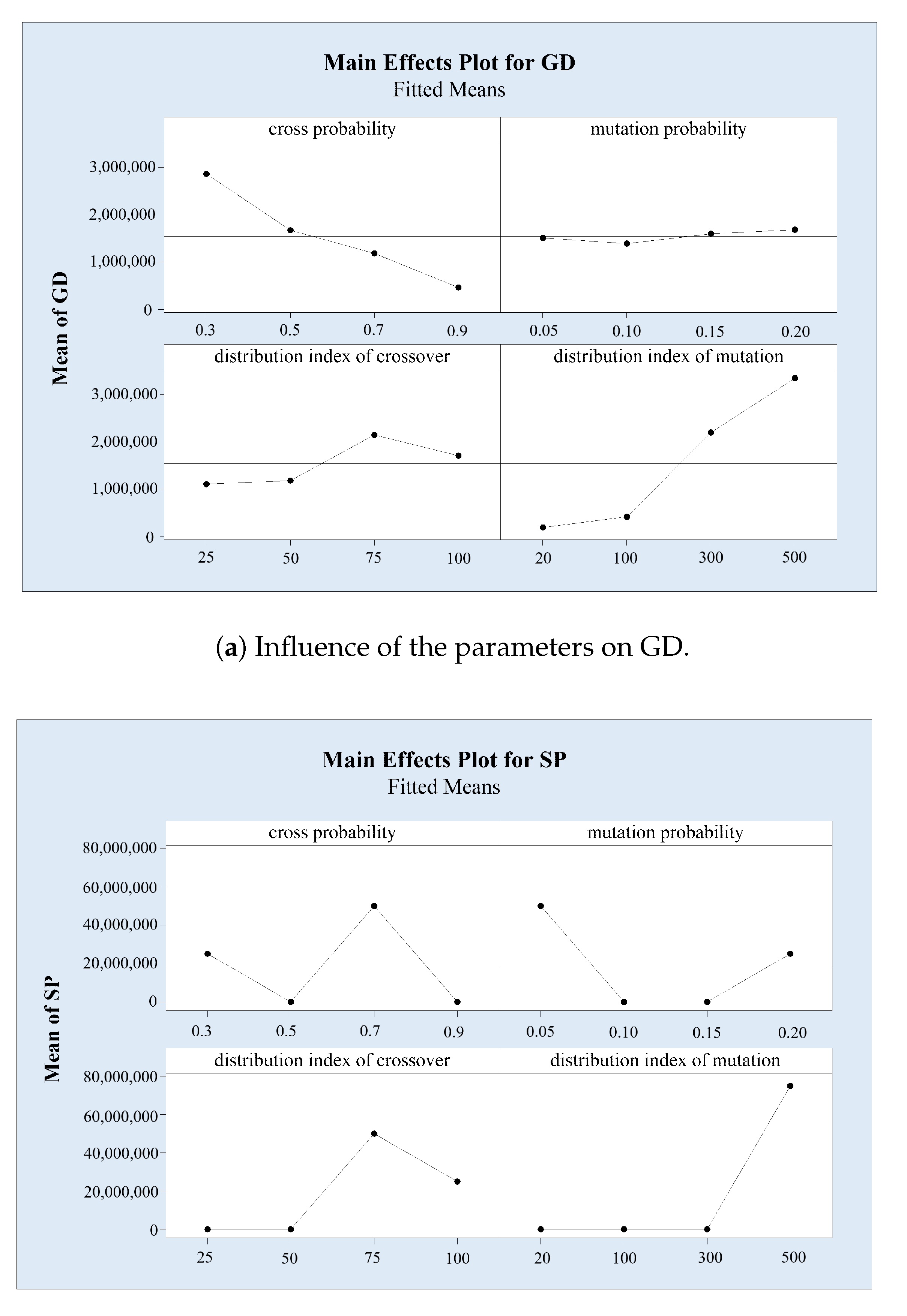
The adopted DOE approach was based on the Taguchi method [18]. All the parameter settings for MOPSO and MOPSO-LS were the same. The details of parameters are shown in Table 3. We also performed the DOE for the NSGA-II to ensure a fair comparison. For the NSGA-II, we focused on the crossover probability p c , mutation probability p m 2 , crossover distribution index d i c and mutation distribution index d i m . The details are shown in Table 4.
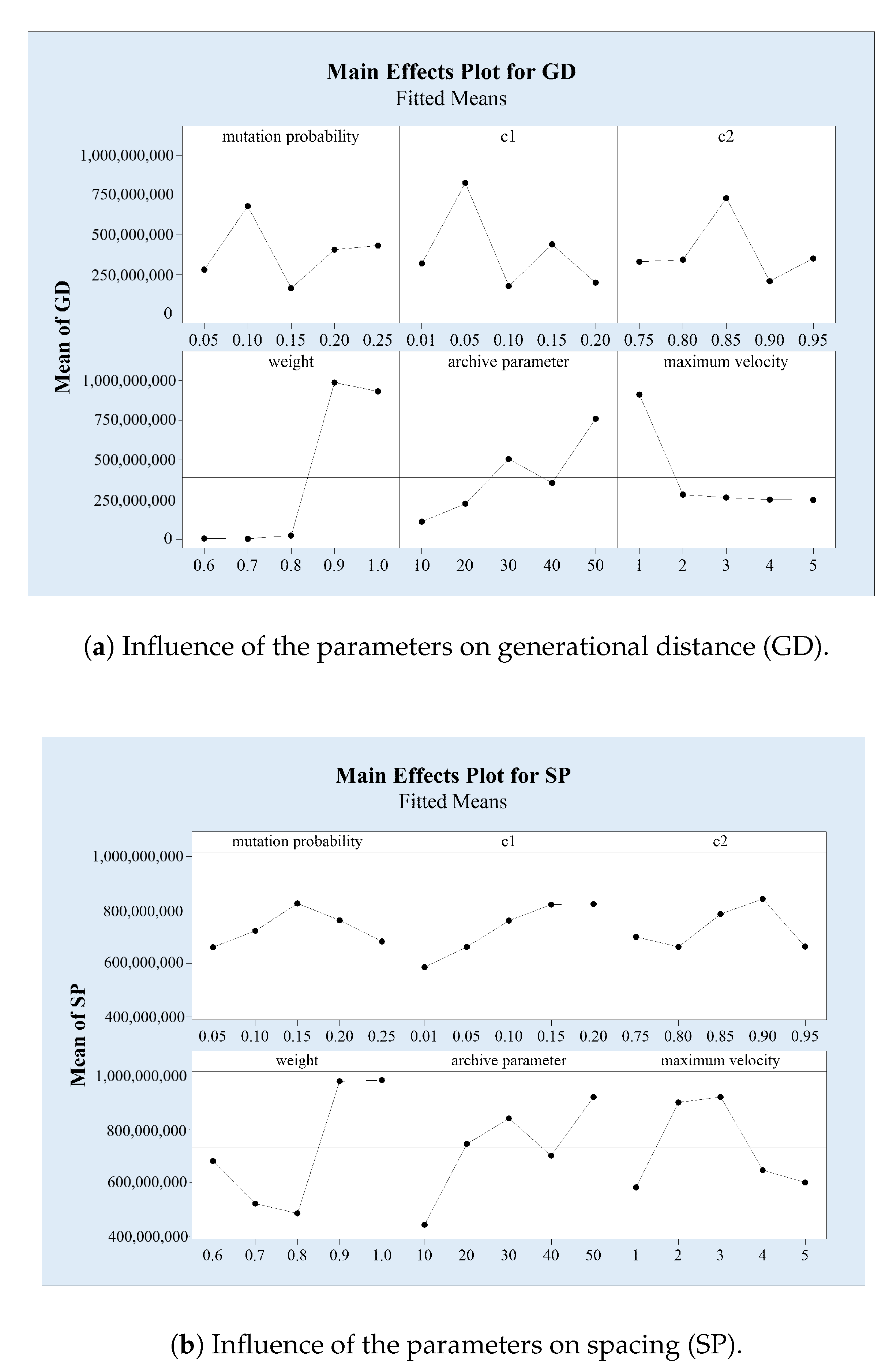
A randomly generated instance with 50 jobs was used in the experiments. For each combination of parameter values, we ran the corresponding algorithm for 10 times and record the average values of GD and SP. The results are shown in Figure 6 and Figure 7. In conclusion, the optimal settings of parameters for MOPSO and MOPSO-LS are as follows: ω = 0.7 , c 1 = 0.1 , c 2 = 0.8 , p m = 0.2 , V max = 3 , n d = 10 . The optimal settings of parameters for NSGA-II are as follows: p c = 0.9 , p m 2 = 0.1 , d i c = 25 , d i m = 20 .

4.4. Performance Comparison

We compared our proposed algorithm MOPSO-LS with MOPSO which excluded the local search function completely. We implemented two-opt, three-opt and four-opt in three versions of MOPSO-LS. Besides, we also compare our algorithm with the well-known multi-objective optimization algorithm NSGA-II [19]. We used the optimal parameter values obtained from the DOE for both algorithms. We have generated instances with 15, 30, 50, 75 and 100 jobs randomly. For each size, 10 different instances have been generated, resulting in 50 test instances in total.
To achieve a fair comparison, we imposed the same computational time limit on all algorithms. The time limits were set as follows: 1 s for 15-job instances, 5 s for 30-job instances, 20 s for 50-job instances, 40 s for 75-job instances and 60 s for 100-job instances. To reduce the impact of randomness, each algorithm was run for 20 independent times on each instance and we record the average result. Table 5 and Table 6 show the results of average GD and SP for each instance.
From the presented results, the following observations and comments can be made:
  • MOPSO-LS shows excellent performance for almost all instances in terms of GD, which suggests that the solutions obtained by MOPSO-LS are closer to the approximate Pareto front. Since all the computational tests are conducted in limited time, we can judge from the table that the convergence speed of MOPSO-LS is much faster than that of MOPSO and NSGA-II, especially for large-scale instances.
  • For some instances, the NSGA-II achieved better results in terms of SP, meaning that the solutions of NSGA-II are distributed more evenly. However, it should be noted that the NSGA-II solutions were located far from the approximate Pareto front, and in this case, the number of non-dominated solutions tends to be much larger and thus it is easier to find evenly spread solutions. Therefore, even though NSGA-II sometimes obtains a better SP, the inferior GD performance indicates worse solution quality.
  • From the table, we can see that the k-opt operator has improved the performance of MOPSO significantly. It is found that three-opt and four-opt are often more powerful than two-opt. However, there is no definite conclusion regarding which one of three-opt and four-opt is more effective (the result appears to be instance-dependent).
To show the results intuitively, we plot the Pareto fronts found by the MOPSO-LS, MOPSO and NSGA-II for an instance with 50 jobs in Figure 8. This figure clearly reveals that our algorithm has obtained much better Pareto fronts than the compared algorithms. It has found solutions with significantly improved total weighted earliness/tardiness and total energy consumption. Noting that earliness/tardiness is an indicator of the manufacturer’s profitability, it is safe to conclude that our algorithm has great potential in improving both profitability and energy efficiency for the manufacturing industry.

5. Conclusions

This paper investigates the single-machine scheduling problem with deterioration to minimize two objectives simultaneously, i.e., the total weighed earliness/tardiness and the total energy consumption. The first objective reflects the just-in-time management philosophy and the second objective reflects the motivation to pursue sustainable and green manufacturing.
We propose a hybrid meta-heuristic algorithm called MOPSO-LS which enhances MOPSO by a dedicated local search procedure to solve the problem. The local search strategy is built on the idea of k-opt neighborhood operators and has been adapted for the scheduling problem. To evaluate the effectiveness and efficiency of the proposed algorithm, computational experiments are conducted and comparisons are made between MOPSO-LS, MOPSO and NSGA-II. The results show that the MOPSO-LS has faster convergence speed and better solution quality compared to the other two algorithms. Besides, it is shown that the local search procedure based on 2-opt, 3-opt and 4-opt have improved the search ability of MOPSO significantly.
In future research, we will focus on more advanced energy models and more sophisticated local search strategies. The energy consumption of machines in different states and the different power rates under adjustable processing speeds will be taken into consideration. This will result in a more complicated scheduling problem with additional decision variables, which makes it necessary to devise an enhanced local search scheme to promote the search efficiency of meta-heuristic algorithms. The k-opt neighborhood operators could be combined with more complex moves to construct an adaptive large neighborhood search policy.

Author Contributions

Conceptualization, Y.L. and R.Z.; methodology, Y.L. and R.Z.; software, X.L.; validation, Y.L., X.L. and R.Z.; formal analysis, Y.L.; investigation, Y.L. and X.L.; resources, R.Z.; data curation, X.L.; writing—original draft preparation, Y.L.; writing—review and editing, R.Z.; visualization, Y.L.; supervision, R.Z.; project administration, R.Z.; funding acquisition, R.Z.

Funding

This research was funded by the Natural Science Foundation of China (grant number U1660202).

Acknowledgments

The authors are grateful to the anonymous reviewers for constructive comments which have helped to improve this paper.

Conflicts of Interest

The authors declare no conflict of interest. The funders had no role in the design of the study; in the collection, analyses, or interpretation of data; in the writing of the manuscript, or in the decision to publish the results.

References

  1. Wang, S.; Liu, M.; Chu, F.; Chu, C. Bi-objective optimization of a single machine batch scheduling problem with energy cost consideration. J. Clean. Prod. 2016, 137, 1205–1215. [Google Scholar] [CrossRef] [Green Version]
  2. Wang, H.; Alidaee, B. Effective heuristic for large-scale unrelated parallel machines scheduling problems. Omega 2019, 83, 261–274. [Google Scholar] [CrossRef]
  3. Plitsos, S.; Repoussis, P.P.; Mourtos, I.; Tarantilis, C.D. Energy-aware decision support for production scheduling. Decis. Support Syst. 2017, 93, 88–97. [Google Scholar] [CrossRef]
  4. Aghelinejad, M.; Ouazene, Y.; Yalaoui, A. Complexity analysis of energy-efficient single machine scheduling problems. Oper. Res. Perspect. 2019, 6, 100105. [Google Scholar] [CrossRef]
  5. Zhang, R.; Chiong, R. Solving the energy-efficient job shop scheduling problem: A multi-objective genetic algorithm with enhanced local search for minimizing the total weighted tardiness and total energy consumption. J. Clean. Prod. 2016, 112, 3361–3375. [Google Scholar] [CrossRef]
  6. Wu, X.; Shen, X.; Li, C. The Flexible Job-Shop Scheduling Problem Considering Deterioration Effect and Energy Consumption Simultaneously. Comput. Ind. Eng. 2019, 135, 1004–1024. [Google Scholar] [CrossRef]
  7. Liao, X.; Zhang, R.; Chiong, R. Multi-objective optimization of single machine scheduling with energy consumption constraints. In Proceedings of the 2017 IEEE Symposium Series on Computational Intelligence (SSCI), Honolulu, HI, USA, 27 November–1 December 2017; pp. 1–8. [Google Scholar]
  8. Módos, I.; Šŭcha, P.; Hanzálek, Z. Algorithms for robust production scheduling with energy consumption limits. Comput. Ind. Eng. 2017, 112, 391–408. [Google Scholar] [CrossRef] [Green Version]
  9. Khorshidian, H.; Javadian, N.; Zandieh, M.; Rezaeian, J.; Rahmani, K. A genetic algorithm for JIT single machine scheduling with preemption and machine idle time. Expert Syst. Appl. 2011, 38, 7911–7918. [Google Scholar] [CrossRef]
  10. Behnamian, J. A parallel competitive colonial algorithm for JIT flowshop scheduling. J. Comput. Sci. 2014, 5, 777–783. [Google Scholar] [CrossRef]
  11. Wang, J.B.; Xia, Z.Q. Flow shop scheduling with deteriorating jobs under dominating machines. Omega 2006, 34, 327–336. [Google Scholar] [CrossRef]
  12. Wang, J.B.; Ng, C.; Cheng, T.E. Single-machine scheduling with deteriorating jobs under a series–parallel graph constraint. Comput. Oper. Res. 2008, 35, 2684–2693. [Google Scholar] [CrossRef]
  13. Wang, J.B.; Liu, L.L. Two-machine flow shop problem with effects of deterioration and learning. Comput. Ind. Eng. 2009, 57, 1114–1121. [Google Scholar] [CrossRef]
  14. Lenstra, J.K.; Kan, A.R.; Brucker, P. Complexity of machine scheduling problems. Ann. Discrete. Math. 1977, 1, 343–362. [Google Scholar]
  15. Coello Coello, C.A.; Pulido, G.T.; Lechuga, M.S. Handling multiple objectives with particle swarm optimization. IEEE Trans. Evol. Comput. 2004, 8, 256–279. [Google Scholar] [CrossRef]
  16. Van Veldhuizen, D.A.; Lamont, G.B. Evolutionary Computation and Convergence to a Pareto Front. 1998. Available online: https://pdfs.semanticscholar.org/f329/eb18a4549daa83fae28043d19b83fe8356fa.pdf (accessed on 1 August 2019).
  17. Schott, J.R. Fault Tolerant Design Using Single and Multicriteria Genetic Algorithm Optimization; Technical Report; Air Force Inst of Tech Wright-Patterson AFB OH: Dayton, OH, USA, 1995. [Google Scholar]
  18. Taguchi, G.; Phadke, M.S. Quality engineering through design optimization. In Quality Control, Robust Design, and the Taguchi Method; Springer: Boston, MA, USA, 1989; pp. 77–96. [Google Scholar]
  19. Deb, K.; Pratap, A.; Agarwal, S.; Meyarivan, T. A fast and elitist multiobjective genetic algorithm: NSGA-II. IEEE Trans. Evol. Comput. 2002, 6, 182–197. [Google Scholar] [CrossRef] [Green Version]
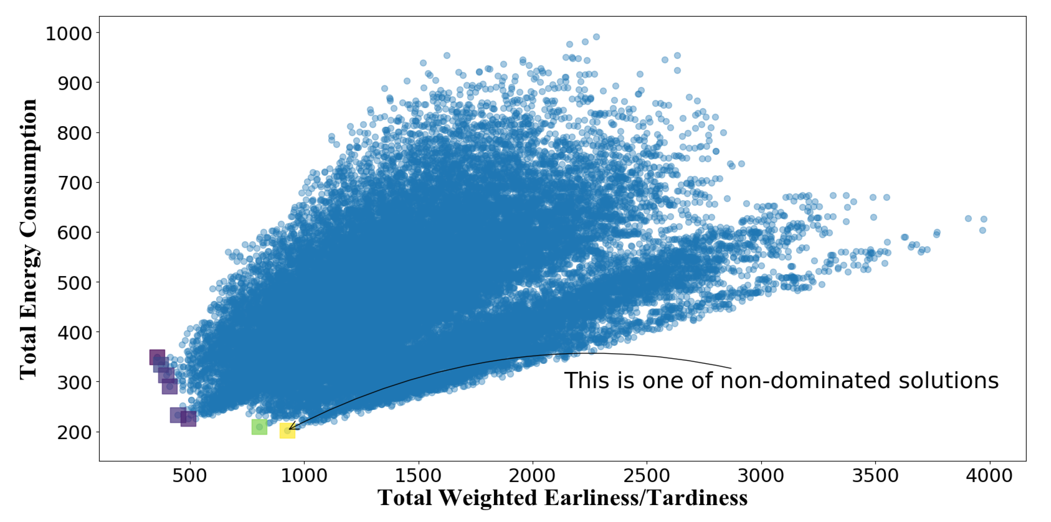
Figure 1. Feasible solutions of the instance.
Sustainability 11 05381 g001
Figure 2. Example of the insertion of a new solution. (a) The case where the inserted individual lies within the boundaries of the grid; (b) The case where the inserted individual lies outside the previous boundaries of the grid.
Sustainability 11 05381 g002
Figure 3. All possible cases for two-opt and three-opt without overlap.
Sustainability 11 05381 g003
Figure 4. Two possible cases for two-opt with overlap.
Sustainability 11 05381 g004
Figure 5. Main steps of the proposed multi-objective particle swarm optimization algorithm enhanced by local search (MOPSO-LS).
Sustainability 11 05381 g005
Figure 6. Influence of the key parameters (MOPSO).
Sustainability 11 05381 g006
Figure 7. Influence of the key parameters (NSGA-II).
Sustainability 11 05381 g007
Figure 8. Pareto fronts for an instance with 50 jobs.
Sustainability 11 05381 g008
Table 1. The job data of a small-scale instance.
j tbp j tls j e j b j d j w j
151230.981853
231620.4282302
3101130.3046295
44610.3868129
56550.2814196
66850.6004155
762130.8456251
872120.8839346
Table 2. Data generation rules.
ItemDistribution
t b p j t b p j u n i f ( 1 , 100 )
b j b j u n i f ( 0 , 1 )
t l s j t l s j 30 × n × u n i f ( 0 , 1 )
d j d j 80 × n × u n i f ( 0 , 1 )
n n { 15 , 30 , 50 , 75 , 100 }
Table 3. Parameters of multi-objective particle swarm optimization (MOPSO).
ParameterValues
ω 0.60.70.80.91
c 1 0.010.050.10.150.2
c 2 0.750.80.850.90.95
p m 0.050.10.150.20.25
V max 12345
n d 1020304050
Table 4. Parameters of NSGA-II.
ParameterValues
p c 0.30.50.70.9
p m 2 0.050.10.150.2
d i c 255075100
d i m 20100300500
Table 5. Comparison of GD.
SizeMOPSO-LSMOPSONSGA-II
2-opt3-opt4-opt
15145.84147.43154.49152.77169.78
21.5359.3277.89111.2160.28
545.36696.60625.72654.69511.43
73.5221.6621.6614.0452.05
36.2720.1741.1055.28126.85
99.6187.3673.2590.70105.44
122.172.2268.3180.0184.22
37.6612.3113.2011.2036.02
87.2125.8111.9224.52158.49
604.48463.84569.45374.33458.47
30 2.1648 × 10 4 2.2128 × 10 4 1.5035 × 10 4 1.4928 × 10 4 2.1667 × 10 4
8193.224345.534005.724149.825625.59
1.4307 × 10 4 9405.306565.11 1.1149 × 10 4 1.0322 × 10 4
2379.981827.372465.722471.712638.53
1769.88780.76510.60972.3191395.41
1315.261047.491730.21788.3712700.17
449.75129.74145.05104.15129.403
1452.09701.53916.551460.242258.18
2815.462088.302770.653052.562385.77
4152.916286.435394.634709.275571.63
50 2.4606 × 10 5 4.2319 × 10 4 1.5017 × 10 5 1.4646 × 10 5 3.1633 × 10 5
1.5841 × 10 5 3.7033 × 10 4 1.6799 × 10 5 7.4834 × 10 4 2.3097 × 10 5
8.9408 × 10 4 1.5656 × 10 4 1.5108 × 10 3 1.9780 × 10 4 5.7527 × 10 4
2.3562 × 10 5 1.8707 × 10 5 2.7467 × 10 5 2.5441 × 10 5 1.0424 × 10 6
5.3550 × 10 5 2.7078 × 10 5 1.9046 × 10 5 1.0054 × 10 5 2.5288 × 10 5
8.5408 × 10 4 3.2339 × 10 4 3.5045 × 10 4 3.4800 × 10 4 1.2134 × 10 5
3.1910 × 10 6 1.1548 × 10 6 8.6985 × 10 5 8.7030 × 10 5 2.2923 × 10 6
8.3748 × 10 4 3.9804 × 10 4 4.9790 × 10 4 1.0186 × 10 5 2.8793 × 10 5
4.0740 × 10 4 3.2010 × 10 4 1.4530 × 10 4 3.7103 × 10 4 8.6083 × 10 4
1.3604 × 10 5 6.9314 × 10 4 6.2159 × 10 4 1.2000 × 10 5 3.2437 × 10 5
75 4.5906 × 10 6 2.1652 × 10 6 1.4288 × 10 6 1.2277 × 10 6 1.8120 × 10 7
2.2032 × 10 6 6.4579 × 10 5 4.5555 × 10 5 3.3948 × 10 5 1.5677 × 10 6
2.1880 × 10 7 1.7321 × 10 6 4.5183 × 10 6 1.7686 × 10 6 1.0907 × 10 7
5.5364 × 10 6 1.1967 × 10 6 1.6280 × 10 6 4.5202 × 10 6 2.6854 × 10 6
1.3444 × 10 7 4.7408 × 10 6 6.0663 × 10 6 5.9801 × 10 6 1.0960 × 10 7
2.0739 × 10 7 1.6263 × 10 7 8.4651 × 10 6 5.1385 × 10 6 1.8489 × 10 7
1.4914 × 10 6 2.8136 × 10 5 5.6996 × 10 5 3.2942 × 10 5 6.8251 × 10 6
1.2989 × 10 7 2.3287 × 10 6 2.3835 × 10 6 9.4526 × 10 5 7.8694 × 10 6
2.6751 × 10 6 5.6586 × 10 5 6.2739 × 10 5 7.4984 × 10 5 3.2544 × 10 6
2.1917 × 10 7 9.9992 × 10 6 9.0490 × 10 6 5.8964 × 10 6 3.4006 × 10 7
100 9.0453 × 10 7 5.2840 × 10 6 1.6884 × 10 7 1.3406 × 10 7 1.2505 × 10 7
4.2289 × 10 7 5.2945 × 10 6 9.3751 × 10 6 1.5119 × 10 7 2.6534 × 10 7
2.2366 × 10 9 3.8023 × 10 8 1.8254 × 10 9 1.0585 × 10 9 3.3249 × 10 9
1.7385 × 10 8 2.5784 × 10 7 2.1698 × 10 7 8.0410 × 10 7 3.1927 × 10 7
4.1691 × 10 7 4.6599 × 10 6 7.6225 × 10 5 2.4933 × 10 6 2.3261 × 10 7
7.6401 × 10 7 2.4467 × 10 7 7.6188 × 10 7 3.6526 × 10 7 5.4984 × 10 8
1.6481 × 10 8 1.1901 × 10 8 1.8326 × 10 8 1.5697 × 10 8 1.2890 × 10 9
6.0461 × 10 8 2.5830 × 10 8 6.7275 × 10 7 4.4045 × 10 7 3.4358 × 10 9
4.2615 × 10 8 6.8537 × 10 7 9.9766 × 10 7 2.9546 × 10 7 6.3862 × 10 8
5.1326 × 10 9 7.6756 × 10 8 5.1069 × 10 8 1.4917 × 10 9 9.7009 × 10 9
Table 6. Comparison of SP.
SizeMOPSO-LSMOPSONSGA-II
2-opt3-opt4-opt
15509.19578.29584.30638.47923.56
417.51435.21555.21477.75444.19
307.09267.71366.51283.58318.55
523.81363.69363.69369.30355.70
1011.111125.71081.631147.831119.74
306.20188.57300.31232.26209.33
357.33373.69342.90414.66245.61
315.46207.31246.36222.78164.90
514.11481.24447.95453.79492.89
517.20367.61413.56686.38452.984
302100.791814.011698.641655.261165.11
6485.565272.554262.614490.446924.92
2165.401275.671412.011486.20778.504
2766.031390.191524.811583.831093.13
1284.55752.24738.56859.83557.49
1677.261111.531202.811068.90992.56
1937.24875.54913.88944.60709.31
5533.602317.052425.592530.012158.28
1819.30934.221027.82944.33596.92
4243.482499.022055.341927.151582.82
50 1.2823 × 10 5 4.0749 × 10 4 6.3635 × 10 4 5.5120 × 10 4 6.5409 × 10 4
4.8729 × 10 4 1.8799 × 10 4 2.2274 × 10 4 3.4729 × 10 4 2.1513 × 10 4
8.3555 × 10 3 4.1071 × 10 3 2.7870 × 10 3 3.4798 × 10 3 1.0090 × 10 4
1.0361 × 10 5 4.9401 × 10 4 5.1010 × 10 4 4.9039 × 10 4 1.0937 × 10 5
2.0716 × 10 4 3.2689 × 10 4 2.0739 × 10 4 3.3511 × 10 4 1.6816 × 10 4
4.1577 × 10 4 2.1366 × 10 4 1.1711 × 10 4 1.0623 × 10 4 1.9758 × 10 4
4.9620 × 10 5 3.7802 × 10 5 2.3289 × 10 5 1.8961 × 10 5 5.9416 × 10 5
6.8611 × 10 4 3.2026 × 10 4 1.3416 × 10 4 3.1120 × 10 4 4.2603 × 10 4
2.8763 × 10 4 1.2816 × 10 4 1.0761 × 10 4 1.2676 × 10 4 1.1313 × 10 4
1.1180 × 10 5 3.2213 × 10 4 2.4039 × 10 4 7.6251 × 10 4 6.3371 × 10 4
75 8.2139 × 10 5 3.1320 × 10 5 2.1188 × 10 5 1.8545 × 10 5 1.7680 × 10 6
2.4810 × 10 5 6.7156 × 10 4 5.8004 × 10 4 1.5406 × 10 5 1.7449 × 10 5
2.7678 × 10 6 2.4515 × 10 5 1.4072 × 10 6 1.3681 × 10 6 1.7745 × 10 6
5.0937 × 10 5 2.8875 × 10 5 2.1010 × 10 5 1.1063 × 10 6 3.2958 × 10 5
2.3024 × 10 6 9.0459 × 10 5 1.2373 × 10 6 1.1083 × 10 6 1.2357 × 10 6
1.6779 × 10 6 4.4779 × 10 5 1.7220 × 10 6 4.9882 × 10 5 1.6083 × 10 6
2.8209 × 10 5 7.5955 × 10 4 8.7421 × 10 4 6.9395 × 10 4 6.0464 × 10 5
3.3010 × 10 6 2.7282 × 10 5 7.2861 × 10 5 2.8029 × 10 5 6.7773 × 10 5
1.1634 × 10 5 5.0719 × 10 4 6.6612 × 10 4 6.8837 × 10 4 1.8110 × 10 5
5.1115 × 10 6 3.3516 × 10 6 2.2598 × 10 6 2.1649 × 10 6 5.4228 × 10 6
100 3.0893 × 10 6 1.0378 × 10 6 2.8150 × 10 6 4.8964 × 10 5 3.3332 × 10 6
3.3866 × 10 6 3.8091 × 10 5 4.1121 × 10 5 1.1611 × 10 6 2.7173 × 10 6
3.5322 × 10 6 1.8074 × 10 7 1.8546 × 10 7 8.8837 × 10 5 1.2989 × 10 6
4.0513 × 10 6 2.2268 × 10 6 6.5448 × 10 6 5.2987 × 10 7 4.2246 × 10 6
4.8506 × 10 6 4.2216 × 10 5 2.1611 × 10 5 1.1851 × 10 5 3.9152 × 10 6
1.4778 × 10 7 3.1322 × 10 6 1.0099 × 10 7 3.2020 × 10 6 3.3094 × 10 6
1.5716 × 10 7 1.4263 × 10 7 3.7640 × 10 7 3.7561 × 10 6 3.5944 × 10 6
1.7767 × 10 7 8.0118 × 10 6 3.8425 × 10 7 7.1203 × 10 6 4.9552 × 10 6
1.7079 × 10 7 3.7224 × 10 6 9.1961 × 10 6 4.0269 × 10 6 1.8599 × 10 6
2.1737 × 10 6 9.5046 × 10 6 3.3712 × 10 6 1.7927 × 10 7 1.1332 × 10 6