Analysis of Agricultural Commodities Prices with New Bayesian Model Combination Schemes

Abstract

In the described research three agricultural commodities (i.e., wheat, corn and soybean) spot prices were analyzed. In particular, one-month ahead forecasts were built with techniques like dynamic model averaging (DMA), the median probability model and Bayesian model averaging. The common features of these methods are time-varying parameters approach toward estimation of regression coefficients and dealing with model uncertainty. In other words, starting with multiple potentially important explanatory variables, various component linear regression models can be constructed. Then, from these models an averaged forecast can be constructed. Moreover, the mentioned techniques can be easily modified from model averaging into a model selection approach. Considering as benchmark models, time-varying parameters regression with all considered potential price drivers, historical average, ARIMA (Auto-Regressive Integrated Moving Average) and the naïve forecast models, the Diebold–Mariano test suggested that DMA is an interesting alternative model, if forecast accuracy is the aim. Secondly, the interpretation of time-varying weights ascribed to component models containing a given variable suggested that economic development of emerging BRIC economies (Brazil, Russia, India and China) is recently one of the most important drivers of agricultural commodities prices. The analysis was made on the monthly data between 1976 and 2016. The initial price drivers were various fundamental, macroeconomic and financial factors.

1. Introduction

Forecasting of agricultural commodities is an important theoretical and practical topic. In 2008 a sudden spike in commodities (in general) prices was observed. Shortly afterwards, these prices had fallen. Nevertheless, since approximately 2000, it can be observed that there exists a rising trend in agricultural prices. This can be clearly seen from analyzing, for example, IMF (International Monetary Fund) commodity food price index, including cereal, vegetable oil, meat, seafood, bananas, sugar and orange prices [1].

These prices are important, because in some developing countries rising food prices or its shortages can lead to riots and increase political and economic uncertainty [2]. Moreover, these prices have a significant impact on farmers. As a result, they are an important component in policymaking and sustainable development [3].

There is also a discussion on what factors influence agricultural prices. It is quite natural to consider in this context natural conditions like the weather. Indeed, these prices are largely influenced by unpredictable droughts, floods and diseases. In this sense forecasting agricultural prices is a hard topic, because these factors are hard to include in the model [4].

Secondly, more conventional economic factors also influence agricultural prices. Of course, this starts from supply and demand forces, as for every tradable good. On the other hand, there exist arguments that interest rates and exchange rates also influence them. Moreover, in recent years there has been a discussion on “financialization” of commodities markets. In other words, the links between spot commodities prices and financial markets are tightening [5,6]. On the other hand, Amann et al. analyzed the causality in Granger sense between volume traded and open positions on derivatives markets and selected agricultural commodities prices (corn, wheat, rice and soybean). They did not find any evidence for such a relationship [7].

There are also arguments that rising crude oil prices impact the transportation costs, and therefore, impact also particular commodities [8].

As a result, building an econometric model for agricultural commodities prices is quite hard, because all the potentially important price drivers are volatile by their own. For example, modelling fluctuations of oil price itself consists of extensive literature. Economic growth in China and other Asian countries highly impacted the agricultural goods demand, etc. [9].

Most of the already applied methods of forecasting focus on a univariate time-series model, like ARIMA, or GARCH-type models (Generalized Auto-Regressive Conditional Heteroskedasticity) in case of volatility modelling [3,10]. More sophisticated approaches are based on neural networks methods, etc. [11]. Another approach is to use structural models [12]. However, in the case of models with multiple explanatory variables, classical regression analysis is mostly used [13].

These conventional econometric methods have two significant drawbacks. First, they require the narrowing of the set of potentially important explanatory variables to quite a small number. Secondly, they assume that during the whole analyzed period, there exists one “true” model. Of course, out of few competing models the final one can be selected. For example, based on fitting the data in the training period. Unfortunately, such an approach omits the fact that during different periods, the “true” model might change. Except that, for traditional models it is harder to capture possible non-linearities [14,15]. Besides, there is a need for more developed econometric models, as the already applied ones usually have poor forecasting performance [16]. In addition, the mentioned methods are not able to capture the time-varying influence of several possible factors on the agricultural prices.

Quite a natural solution comes from Bayesian econometrics. However, these methods have not been applied yet too extensively to modelling agricultural prices [17], despite the fact, that they seem to be quite useful in this context [18,19]. Therefore, the current paper was an attempt to fill this literature gap.

Herein, dynamic model averaging (DMA) introduced by Raftery et al. was applied to forecasting selected agricultural prices [20]. The advantage of this method is that it takes under consideration uncertainty about the “true” model. Therefore, in the beginning stage several potentially important explanatory variables could be inserted into the modelling scheme.

Secondly, the conventional limitations over the ratio of explanatory variables to the length of time-series do not apply for this method [21].

Third, this method is based on recursive computations, which resembles the real-market conditions, when forecasting can be done only on the basis on the past information; but in the next period the model can (and should) be updated (re-estimated), because new (more) information is available. For example, the mentioned impact of crude oil price on agricultural commodities can be asymmetric, i.e., positive and negative oil price shocks can differently influence agricultural commodities prices [22], which suggests that econometric model with time-varying regression coefficients might be desirable.

Finally, the weights ascribed to each of the component model are time-varying. This allows for certain economic interpretation of time-varying importance of the included explanatory variables [23]. Indeed, it seems that time-varying methods have still not been much applied to analysis of agricultural commodities markets [24].

In addition, this scheme can be easily modified into model selection. Herein, this was done in two ways. As commonly, the selected model was the one with the highest posterior probability. Additionally, the scheme of, so called, Median Probability Model (MPM) by Barbieri and Berger was considered [25].

This paper is organized in the following way. First, a literature review on agricultural commodities prices drivers is presented. Next, the dataset is described and the motivation for particular data proxies is given. For the reader’s convenience a short exposition of dynamic model averaging is sketched; and the used methodology is described. Finally, the obtained results are presented and discussed.

2. Literature Review

Rezitis and Sassi provided an extensive review of various drivers of agricultural commodities prices in the time-varying context [26]. They covered mostly the period between 1996 and 2008. During all this time fundamental factors (like supply and demand) played an important role in impacting agricultural prices. These come from a rise in demand due to growth of population, rapid economic growth and rise in per capita consumption.

Within this context usually the economic growth in BRIC countries is highlighted, as the individual welfare in these countries is rising, as well as their urban population, making significant changes in consumption patterns [27].

Of course, these changes were followed by the strong growth in production. However, around 2000 it was observed that the demand for stocks was declining. Since 2000 there is also growing concern about the impact of rising crude oil prices and U.S. dollar devaluation. Since 2006 researchers have also focused on rising input costs, adverse weather, aggressive purchases by importers, export bans and restrictions and import tariff reductions.

Rezitis and Sassi [26] presented also a discussion of complicated grains commodities price formation. In short, energy policies impact crude oil prices, which further impacts biofuels and ending stocks, which finally has an impact of the demand. For example, increase in demand for crops for biofuels can result in substitution effect and increase competition in using the land [28].

Bastianin, Galeotti and Manera [29] analyzed the relationship between ethanol prices and certain grain prices. They do not find a causal relationship from ethanol return to food prices. Moreover, Zilberman et al. also stated that biofuel prices do not impact food commodities price, but the introduction of biofuels does [30]. For example, Paris concluded that both non-linearities and regime switching should be considered when analyzing impact of biofuels on agricultural prices [31]. In particular, it was found that biofuels expansions can lead to higher agricultural commodities prices. Therefore, it can be said that the relationship between biofuel prices and agricultural commodities prices is not conclusively solved in literature. Sometimes, different outcomes are found depending on whether a global level or national one is analyzed [32,33].

Weather conditions, harvest area, cost of oil and fertilizers and beginning stocks have an impact on the supply side. Indeed, higher energy and fertilize prices result in higher production and transportation costs. However, the nature of links between crude oil price and agricultural commodities prices is disputable, whether it is mostly driven by common macroeconomic determinants of both prices, or it is a direct pass-through [34].

Both, conventional statistical methods and Bayesian ones, provide much evidence that crude oil price improves the forecasting performance of modelling agricultural prices [19]. Indeed, Nazlioglu and Soytas concluded that both crude oil price and exchange rates impact agricultural commodities prices in the sense of Granger causality [35]. They found that there are significant interactions between crude oil and corn prices, but not between crude oil and soybean prices and between crude oil and sugar prices. Such interdependencies were also found by Fernandez-Diaz and Morley [36].

Sukcharoen and Leatham [37] argued that regime switching should be included when analyzing the relationship between crude oil and agricultural commodities prices. In particular, they found that the statistical dependence between these commodities is high during market downturns, but not during market upturns.

The level of stocks is also impacted with both production shortfalls and political decisions. For example, some net exporting countries introduced restrictive trade policies. For example, around 2008 China, India, Russia, Ukraine and Argentina raised their export taxes [38].

Ribeiro and Oliveira [14] noticed the important role of stocks quotas in predicting agricultural commodities prices. However, they provided an analysis confirming that the convenience yield can be a more important explanatory variable in modelling these commodities prices. In fact, this factor is connected with supply shortages. It is a kind of a premium from holding the good over holding a derivative position [39].

Moreover, exchange rates have an important impact on foreign demand; whereas export restrictions impact upon foreign supply. Of course, adverse weather conditions result in production shortfalls, impacting lower level of supply and stocks. These can have also a relationship with precautionary purchases, which constitutes a part of demand. Besides, grain reports and future markets have impact on price expectations, which also impact both demand and supply. However, these expectations also impact directly both supply and demand [26].

Chen, Rogoff and Rossi [40] analyzed world agricultural prices. They found that factors like stock market indices and exchange rates can improve the predictability of agricultural prices. The theoretical argument in favor of this conclusion is that financial markets are more fluid than agricultural markets, so the information from them can be used as a signal of some future agricultural price dynamics. Also, Thiyagarajan et al. found that stock markets and exchange rates have a significant impact on the prices of agricultural commodities in India [3].

Fernandez-Diaz and Morley [36] found significant interdependence between soybean price and U.S. exchange rate and between sugar prices and global economic activity. Also, Alam and Gilbert observed the important role of global economic conditions for development of agricultural commodities prices [41]. However, Hatzenbuehler et al. found that stocks quotas and policy shifts are more important in affecting long-term agricultural prices than exchange rates, because they give rise to more inelastic market demand [42]. However, in the short-term the effect can be opposite, i.e., exchange rates can play a more important role.

3. Data

The analyzed period covered the span between July 1976 and July 2016. Such a choice was due to the data availability. Monthly or yearly frequency was taken depending also on data availability.

Prices of agricultural commodities were taken from The World Bank [43] in $/mt. Following, for example, Kapusuzoglu and Karacer Ulusoy, wheat (U.S. HRW), corn (maize) and soybean prices were collected (P_WHEAT, P_CORN, P_SOYBEAN) [44]. This data is provided in monthly frequency.

Production (prefixed with Q_), consumption (prefixed with D_) and (ending) stock quotas (prefixed with S_) estimates were taken from O’Brien [45], which is a collection of regularly published [46] reports. Production, consumption and stocks were taken in million metric tons. These data were provided in yearly frequency. Moreover, the marketing year for these agricultural commodities depends on country. However, for the world data it can be assumed that it goes from July to July.

Exchange rates were taken from Stooq [47] and FRED [48]. Following Chen et al. [40], Australian dollar (AUD) and Canadian dollar (CAD) to U.S. dollar rates were taken. The mnemonic time-series are AUDUSD from Stooq [47] for AUD and EXCAUS for CAD from FRED [48]. The motivation behind this was that these two countries are important producers (and exporters) of the analyzed commodities. They have had open markets and free-floating currency regimes for long time. Their economies are also developed ones and quite stable. On the other hand, other important exporters (Argentina, Brazil, China and Russia) suffered serious crises, hyper-inflation, etc. These time-series are provided in monthly frequency.

Market stress index (MS) was taken as Moody’s seasoned Baa corporate bond minus federal funds rate [48]. This data is provided in monthly frequency. FRED [48] mnemonic time-series is BAAFFM. The idea is to consider the difference between “risky” asset and a “risk-free” one [49].

As an interest rate (R) long-term government bond yields: 10-year: main (including benchmark) for the United States were taken. The mnemonic [48] time-series is IRLTLT01USM156N. This data is provided in monthly frequency.

Stock market index was taken as S and P 500 from Stooq [47]. The mnemonic time-series is SPX. This data is provided in monthly frequency.

Traditional biofuels production (in terrawatt-hours) was taken from Ritchie and Roser [50]. It was denoted by BIO. This data is provided in yearly frequency.

Energy prices (E) were also taken from The World Bank [43]. For the oil price (OIL) the average from Brent, Dubai and WTI (West Texas intermediate) was taken, as provided by The World Bank [43] in $/bbl. This data is provided in monthly frequency.

Fertilizer prices (F) were also taken from The World Bank [43] in nominal U.S. dollars. This data is provided in monthly frequency.

Global economic activity (KEI) was taken as the Kilian index [51,52]. This index is based on ocean bulk dry cargo freight rates [53,54]. Such an index has certain advantages in measuring real global economic activity over, for example, considering global real GDP or industrial production measures. The Kilian index was constructed to meet several goals. First, to cover global activity. Secondly, to account that in many countries service sector increases as a part of their GDP. Third, to construct a measure that captures real activity—not coincidental factors. In addition, the Kilian index is regularly updated and provided in monthly frequency, and dates back to 1968.

Annual growths of GDP per capita from BRIC countries were taken from The World Bank [55]. Then, the mean values from all four countries were taken to obtain one time-series (GDP). These data are provided in yearly frequency. Moreover, Russia is included in this collection since 1990.

Following, for example, Buncic and Moretto [39], convenience yield (prefixed with CY_) was computed as

$$\mathrm{CY}=\mathrm{rf}-\left(\mathrm{Fp}-\mathrm{P}\right)/\mathrm{P},$$

(1)

where rf stands for risk-free rate, Fp—for futures price, and P—for spot price. Of course, futures price and risk-free rate should correspond to the same time horizon. Risk-free rate, for this computation, was taken as three-month treasury bill: secondary market rate [48]. The mnemonic time-series is TB3MS. Futures prices were taken from Stooq [47]. The mnemonic time-series are KE.F for wheat, ZC.F for corn and ZS.F for soybean. They are provided in ¢/bu. However, spot prices were collected in $/mt. Therefore, simple re-calculations were done, assuming that one bushel of wheat equals to 27.2155 kg, one bushel of corn equals to 25.4012 kg, and one bushel of soybean equals to 27.2 kg [56]. All these data are provided in monthly frequency.

Open interest (OP_) was also taken for each grain from Stooq [47]. It represents the sum of all contracts that have not expired, i.e., it shows the number of long (or equivalently: short) positions. This indicates the activity of futures market and can be used for measuring speculative pressures [7]. These data are provided in monthly frequency.

Because the time-series were in different frequencies, the yearly ones were disaggregated into monthly ones. Of course, disaggregation resulted in lower accuracy of the resulting time-series, but it seemed that such a bad time-series was preferable to switching all data into lower frequency. Indeed, the majority of time-series are in monthly frequency, including the dependent variables. On the other hand, the very interesting and important time-series (like, for example, production and consumption) are in yearly frequency. Therefore, it seems worth to make this procedure. It was done with the help of “tempdisagg” R package [57]. The Denton–Cholette method was used because the time-series contained trends and in order not to deal with stationarity or cointegration issue,.

In particular, BIO was disaggregated in a way to keep the yearly sums consistent with the original time-series. Similarly, time-series of production, consumption and stocks. However, for GDP the aim was to keep yearly means consistent with the original time-series. Actually, in this case geometric mean would be even more desirable, but such a disaggregation was not available in the applied package.

It was desirable for all variables to have more or less similar magnitudes. Therefore, KEI and production, consumption and stock quotas were divided by 100. Such a re-scaling does not change the economic meaning, just the quantities measures considered.

Moreover, prices and S and P 500 stock market index (SP500) were transformed to returns (i.e., monthly growths). For consumption, production and stocks the ordinary first differences (i.e., differences between subsequent months) were taken. For open interest, exchange rates, oil price, energy price, fertilizer prices and biofuels production the monthly growths were taken.

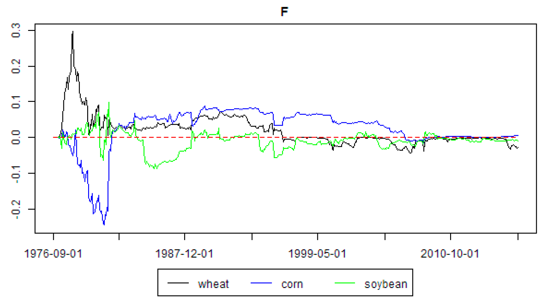
The descriptive statistics of the variables, after the above transformations, are presented in

Table 1. Descriptive statistics of time-series after the transformations.

	Mean	SD	Variance	Min	Max	Skew	Kurtosis
P_WHEAT	0.0017	0.0572	0.0033	−0.1968	0.2575	0.7822	3.1160
D_WHEAT	0.0006	0.0011	0.0000	−0.0036	0.0044	−0.0278	0.6676
Q_WHEAT	0.0007	0.0032	0.0000	−0.0083	0.0098	0.1677	0.0975
S_WHEAT	0.0003	0.0018	0.0000	−0.0043	0.0053	0.0432	−0.3567
OP_WHEAT	0.0638	0.3602	0.1298	−0.7142	1.3980	0.6731	0.4122
CY_WHEAT	0.1044	0.0566	0.0032	−0.2655	0.2488	−1.1140	4.3320
P_CORN	0.0023	0.0587	0.0035	−0.2172	0.3465	0.3273	3.6120
D_CORN	0.0011	0.0016	0.0000	−0.0030	0.0084	0.6266	1.9940
Q_CORN	0.0011	0.0045	0.0000	−0.0139	0.0153	0.1631	0.9350
S_CORN	0.0015	0.0037	0.0000	−0.0111	0.0169	0.2704	1.9660
OP_CORN	0.0100	0.0975	0.0095	−0.2742	0.4806	1.0140	2.5020
CY_CORN	0.0928	0.0611	0.0037	−0.1257	0.3678	0.5115	1.9460
P_SOYBEAN	0.0025	0.0545	0.0030	−0.2390	0.2890	0.3194	3.7330
D_SOYBEAN	0.0005	0.0006	0.0000	−0.0014	0.0021	0.1251	0.0728
Q_SOYBEAN	0.0005	0.0014	0.0000	−0.0034	0.0054	0.3755	0.4194
S_SOYBEAN	0.0001	0.0006	0.0000	−0.0023	0.0018	−0.1599	0.8353
OP_SOYBEAN	0.0173	0.2393	0.0573	−0.7681	4.6230	14.8000	283.5000
CY_SOYBEAN	0.1129	0.0536	0.0029	−0.1148	0.2782	−0.5024	2.1460
BIO	0.0002	0.0008	0.0000	−0.0014	0.0018	−0.3993	−1.4340
GDP	0.0388	0.0239	0.0006	−0.0099	0.0921	0.0231	−0.7001
MS	0.0358	0.0198	0.0004	−0.0405	0.0882	−0.7334	1.2110
KEI	0.0105	0.5537	0.3066	−1.6340	1.8790	0.8715	1.2510
SP500	0.0073	0.0429	0.0018	−0.2176	0.1318	−0.6003	2.0520
R	0.0654	0.0317	0.0010	0.0150	0.1532	0.5573	−0.2871
AUD	−0.0005	0.0329	0.0011	−0.1776	0.1048	−0.7338	3.6420
CAD	−0.0005	0.0152	0.0002	−0.1068	0.0619	−0.3558	5.5340
OIL	0.0063	0.0847	0.0072	−0.3552	0.5379	0.7551	6.9910
E	0.0051	0.0699	0.0049	−0.2838	0.4132	0.5477	5.5630
F	0.0047	0.0740	0.0055	−0.3053	0.8829	3.8740	45.0700

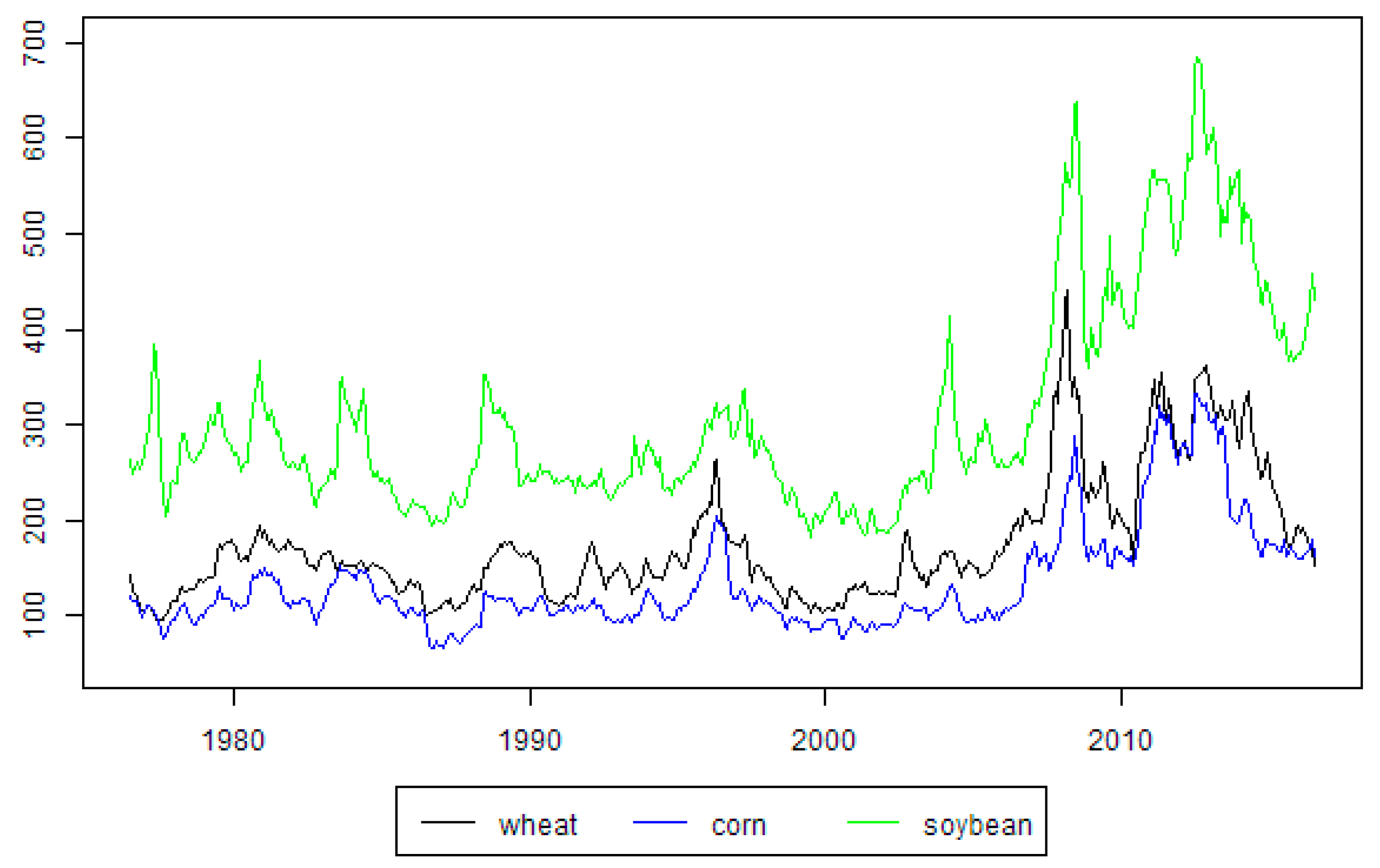
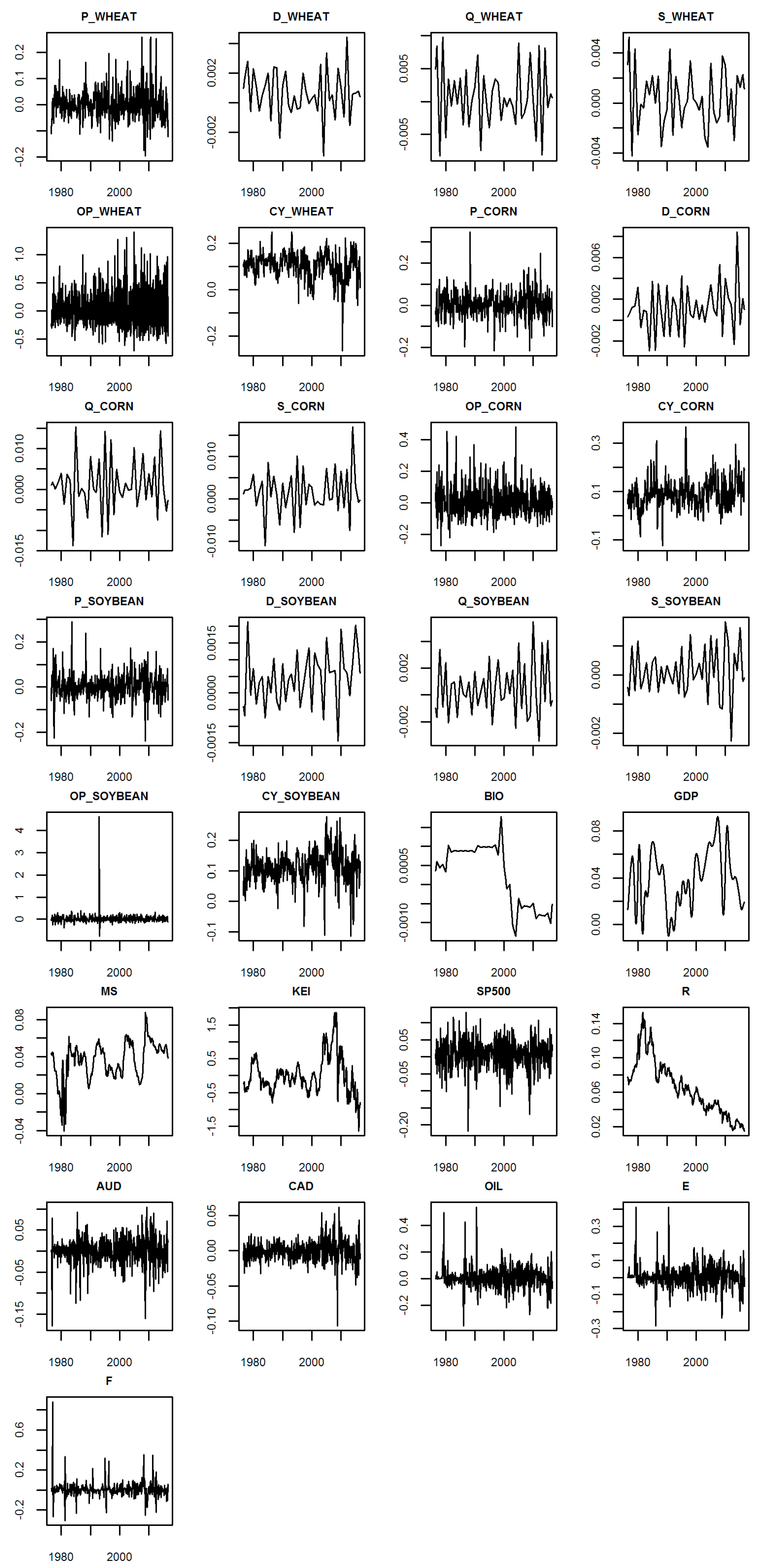
. In Figure 1 the time-series of the selected agricultural commodities are presented. In Figure 2—of all the variables, after the described transformations. For the sake of clarity and readability all variables abbreviations are listed in

Table A1. Abbreviations of variables used.

Abbreviation	Meaning
P_	price
D_	consumption
Q_	production
S_	stocks
OP_	open interest
CY_	convenience yield
BIO	traditional biofuels production
GDP	annual growth of GDP per capital in BRIC countries
MS	market stress index
KEI	Kilian index of global economic activity
SP500	S and P 500 stock market index
R	long-term interest rate
AUD	AUD to USD exchange rate
CAD	CAD to USD exchange rate
OIL	crude oil price
E	energy prices
F	fertilizer prices

in the Appendix A.

4. Methodology

The computations were done in R [58] with the help of “fDMA” and “forecast” packages [59,60].

Dynamic model averaging (DMA) was developed by Raftery et al. [20]. Assuming there are n potentially interesting explanatory variables, one can make 2ⁿ multilinear regression models out of them. In the case presented herein, n = 16 for each of the analyzed agricultural commodities. Let t denote the time index, and let y_t be the dependent variable, and let x_t^(k) be the vector of explanatory variables in the k-th multilinear regression model. Of course, k = 1, …, 2n. For clarity, both y_t and x_t^(k) represent the time-series after the transformations described in the previous section (i.e., those reported in Table 1 and presented in Figure 2). Moreover, independent variables are taken from the one period back comparing to the dependent variable (i.e., in their first lags). This is because the focus in this research was on forecasting the prices. The state space model is given by the following equations:

$$y_t=x_t^{\left(k\right)}{\theta }_t^{\left(k\right)}+{\epsilon }_t^{\left(k\right)},$$

(2)

$${\theta }_t^{\left(k\right)}={\theta }_{t-1}^{\left(k\right)}+{\delta }_t^{\left(k\right)}$$

(3)

with θ_t^(k) denoting the regression coefficients of the k-th multiple linear regression model. Errors are normally distributed, i.e., ε_t^(k) ~ N(0,V_t^(k)) and δ_t^(k) ~ N(0,W_t^(k)).

The regression coefficients are recursively updated by Kalman filter. V₀^(k) and W₀^(k) need to be given the initial values. For specifying W₀^(k) the procedure proposed by Raftery et al. [20] was used. V₀^(k) were set to 1, because they should correspond to magnitudes of the variables, so such a value is in line with their variances reported in Table 1. Further updating depends on a certain forgetting factor λ, which is a number between 0 and 1. The details are presented in the paper by Raftery et al. [20].

Smaller values of λ correspond to allowing more abrupt updating (changes) of θ_t^(k). However, too small values might result in “catching the noise”, instead of “catching the signal”. Therefore, here the most common values [61] were tested, i.e., λ = {1, 0.99, 0.98, 0.95, 0.90}.

As DMA is a model averaging scheme, each of the component k-th multiple linear regression model is given a time-varying weight. This is done through the following equations:

$${\pi }_{t|t-1,k}=\raisebox{1ex}{$\left({\pi }_{t-1|t-1,k}^{\alpha }+c\right)$}\!\left/ \!\raisebox{-1ex}{$\left({{\displaystyle \sum }}_{i=1}^K{\pi }_{t-1|t-1,i}^{\alpha }+c\right)$}\right.,$$

(4)

$${\pi }_{t|t,k}=\raisebox{1ex}{$\left[{\pi }_{t|t-1,k}{f}_k\left(y_t|Y^{t-1}\right)\right]$}\!\left/ \!\raisebox{-1ex}{$\left[{{\displaystyle \sum }}_{i=1}^K{\pi }_{t|t-1,i}{f}_i\left(y_t|Y^{t-1}\right)\right]$}\right.,$$

(5)

where f_k(y_t|Y_t−1) is the predictive density of the k-th model at y_t, under the assumption that the data up to time t is known (but not further), and K = 2ⁿ. Here, also the second forgetting factor α is used. For the economic interpretation it seems that α = λ is a reasonable choice, as then the “tempo” of updating is the same for all parameters of the DMA scheme.

The weights π_t|t−1,k are called posterior predictive probabilities. Raftery et al. [20] advise the use of some small constant c to prevent these probabilities being reduced to 0. This can happen due to numerical approximations during software computations. They recommended setting c = 0.001/2ⁿ.

The values of π_0|0,k need also be given the initial values. So-called non-informative prior was used, i.e., π_0|0,k = 1/2ⁿ were taken. In other words, initially all component models were given the same equal weight.

The DMA prediction is obtained as an averaged forecast with the following equation:

$$\widehat{y_t^{DMA}={\displaystyle \sum }_{k=1}^K{\pi }_{t|t-1,k}\widehat{y_t^{\left(k\right)}}}$$

(6)

where $\widehat{y_t^{\left(k\right)}}$ is the prediction from the k-th multilinear regression model.

If α = 1 = λ, then the above scheme is a computationally efficient way to estimate Bayesian model averaging [20]. This is denoted by BMA.

The model averaging scheme described above can be easily switched to model selection scheme. The usual choice is to select in each time t the model with the highest posterior predictive probability in Equation (6), instead of weighted averaging over all component models. Such a scheme is called dynamic model selection (DMS). Similarly, for α = 1 = λ, the scheme is called Bayesian model selection (BMS).

On the other hand, Barbieri and Berger [25] argued that only under certain conditions the model with the highest posterior probability is the optimal one. Suppose that the weights π_t|t−1,k from exactly those component models, which contain a given explanatory variable, are summed up. Such a sum is called posterior inclusion probability (of this explanatory variable).

Barbieri and Berger [25] proposed to select the component model, which contains exactly those explanatory variables, for which posterior inclusion probability is greater than or equal to 0.5. This scheme is called the median probability model (MED). Similarly, for α = 1 = λ this scheme is called herein the Bayesian median probability model (BMED).

Additionally, posterior inclusion probabilities together with the weighted regression coefficients can be used to describe the time-varying importance of a given explanatory variable in influencing the dependent variable [23]. More precisely, high values of posterior inclusion probability for a given variable should be confronted with the weighted regression coefficient for this variable. High posterior inclusion probability, when the weighted regression coefficient is around 0, does not indicate high importance of this variable as an explanatory variable. In other words, such a situation means that conclusions from individual component models in averaging scheme are opposite to each other.

Of course, it is necessary to compare the forecast accuracies of the analyzed model combination schemes with some benchmark models. Definitely, the common ARIMA model is the first choice. Actually, herein the automatic version of Hyndman and Khandakar [60] is used (ARIMA). In short this model is applied recursively, i.e., data up to time t − 1 are used to make the forecast for time t. Then, data up to time t are used to make the forecast for time t + 1, etc. Moreover, the model initially starts with no AR (Auto-Regressive) and MA (Moving Average) lags and searches if more lags give some improvement according to Akaike Information Criterion.

The next benchmark model is just a naïve forecast (NAÏVE), i.e., forecast for time t is simply the observed value at time t − 1. It is worth mentioning that sometimes, in case of commodities markets, it is a hard task even to make a more accurate forecast than the naïve method [62].

It is also interesting to compare the model averaging and model selection schemes with a single model with time-varying regression coefficients, but with all considered variables as explanatory ones. Indeed, the DMA scheme is described as averaging over K = 2ⁿ time-varying parameters regressions. The scheme can be also considered with no averaging, just as a way of computing time-varying parameters regression, if K = 1, i.e., just one component model is considered. For this model, denoted by TVP, the forgetting factor λ was set to 0.99.

The last benchmark model is to take historical average (HA). In other words, the forecast for time t is the mean from all observations up to time t − 1.

The whole sample was divided into in-sample consisting of the first 120 observations, and out-of-sample consisting of the remaining further observations. In such a way in-sample consisted of 25% of the whole data set. The estimated models were evaluated on the basis of the out-of-sample part. In particular, root mean squared error (RMSE), mean absolute error (MAE) and mean absolute scaled error (MASE) were computed, after deleting first 120 observations. However, the estimated models were directly forecasting the returns from the given agricultural commodity, i.e., it was previously described how the raw time-series were transformed. On the other hand, the forecast accuracy measures were applied to the prices of the analyzed agricultural commodities. It is an easy algebraic transformation, to obtain forecasted prices back from forecasted returns (annual changes).

RMSE and MAE are quite common forecast accuracy measures. RMSE penalizes more extreme discrepancies, as it is based on second power function, whether MAE treats them linearly. Hyndman and Koehler [63] advocated using MASE, which for T observations is defined by the following equation:

$$\mathrm{MASE}=\raisebox{1ex}{${{\displaystyle \sum }}_{t=1}^T|y_t-\widehat{y_t|}$}\!\left/ \!\raisebox{-1ex}{$\left(\frac{T}{T-1}{{\displaystyle \sum }}_{t=2}^T|y_t-y_{t-1}|\right)$}\right.$$

(7)

where y_t represents the real values, and $\widehat{y_t}$ represents the forecasted values. The advantages of this forecast accuracy measure are: scale invariance, “good” behavior if the forecasted values are around 0, penalizing both positive and negative errors equally, penalizing both large and small differences between real and forecasted values equally. Additionally, it has an easy interpretation: values of MASE greater than one indicate that the naïve method is characterized by greater forecast accuracy than the evaluated method.

The estimated models were checked if they generated better forecast accuracy than the benchmark models. However, the stress was put on evaluating the models due to the criterion of minimizing MASE.

It was noticed that MASE, or more precisely the absolute scaled error (ASE) loss function, was compatible with the procedures of the common [64] test. Therefore, except comparing values of MASE for different models, it was also checked if the observed—greater or smaller—forecast accuracy was statistically significant for each case.

5. Results

From

Table 2. Forecast accuracy measures and Diebold–Mariano test outcomes for wheat.

	RMSE	MAE	MASE	DM Test Statistic	DM Test p-Value
DMA (α = 0.99 = λ)	12.3900	8.0010	1.0360	-	-
DMA (α = 0.98 = λ)	12.5300	8.1450	1.0550	1.6330	0.0512
DMA (α = 0.95 = λ)	13.6100	8.9180	1.1550	3.8820	0.0001
DMA (α = 0.90 = λ)	15.2100	9.7820	1.2670	4.7220	0.0000
BMA	12.4900	8.0340	1.0410	0.3766	0.3532
DMS (α = 0.99 = λ)	12.7300	8.2970	1.0750	2.7120	0.0033
DMS (α = 0.98 = λ)	13.1100	8.3620	1.0830	2.4010	0.0082
DMS (α = 0.95 = λ)	14.1700	9.2190	1.1940	4.0960	0.0000
DMS (α = 0.90 = λ)	16.4000	10.1900	1.3190	4.3540	0.0000
BMS	12.9900	8.3440	1.0810	2.1480	0.0158
MED (α = 0.99 = λ)	12.3400	8.0350	1.0410	0.3792	0.3523
MED (α = 0.98 = λ)	12.7600	8.2290	1.0660	1.8150	0.0348
MED (α = 0.95 = λ)	14.0800	9.1750	1.1880	4.0690	0.0000
MED (α = 0.90 = λ)	15.8300	9.8170	1.2710	4.4310	0.0000
BMED	12.7000	8.2140	1.0640	1.7520	0.0399
TVP (λ = 0.99)	12.6200	8.2760	1.0720	2.0000	0.0228
HA	73.5500	49.3700	6.3950	15.5300	0.0000
ARIMA	13.9600	8.8550	1.1470	2.5070	0.0061
NAÏVE	13.8800	8.8800	1.1500	2.5710	0.0051

it can be seen that, in the case of wheat prices, it was DMA with α = 0.99 = λ, which minimized MASE. Interestingly, this was also the model, which simultaneously minimized RMSE out of all the considered models, as well as, minimized MAE. For Diebold–Mariano test 5% significance level was assumed [65]. In such a case, it can be stated that the selected DMA model with α = 0.99 = λ produced significantly more accurate forecasts than the majority of the alternative models. The only exceptions were DMA with α = 0.98 = λ, BMA (i.e., DMA with α = 1 = λ) and MED with α = 0.99 = λ.

This meant that the selected model produced similarly accurate forecast if forgetting factors were slightly larger or smaller. It also seemed not to differ whether model averaging or model selection was applied for the selected forgetting factors. However, if the scheme of Barbieri and Berger [25] is considered, i.e., if not the highest posterior probability model was selected, then forecast accuracies do not differ significantly.

Usually, the time-varying parameter approach (i.e., α, λ < 1) leads to smaller forecast errors, while further lowering of the values of forgetting factors results in increasing forecast errors. This outcome quite confirms the suggestion of Raftery et al. [20] and Koop and Korobilis [66] that the combination of forgetting factors α = 0.99 = λ is preferable. On the other hand, there are applications of DMA, when more subtle combinations worked better [67,68].

From

Table 3. Forecast accuracy measures and Diebold–Mariano test outcomes for corn.

	RMSE	MAE	MASE	DM Test Statistic	DM Test p-Value
DMA (α = 0.99 = λ)	9.3900	5.9120	1.0060	0.4663	0.3205
DMA (α = 0.98 = λ)	9.5910	6.0130	1.0230	1.0990	0.1358
DMA (α = 0.95 = λ)	10.9700	6.5650	1.1170	2.7240	0.0032
DMA (α = 0.90 = λ)	12.5000	7.2180	1.2280	3.5780	0.0002
BMA	9.3390	5.8810	1.0000	-	-
DMS (α = 0.99 = λ)	9.5220	6.0170	1.0240	1.4130	0.0788
DMS (α = 0.98 = λ)	9.7870	6.1730	1.0500	1.8050	0.0355
DMS (α = 0.95 = λ)	11.9000	6.8160	1.1590	2.9740	0.0015
DMS (α = 0.90 = λ)	13.6700	7.6120	1.2950	3.9680	0.0000
BMS	9.3260	5.9330	1.0090	0.7123	0.2382
MED (α = 0.99 = λ)	9.5840	6.0720	1.0330	2.0640	0.0195
MED (α = 0.98 = λ)	10.0200	6.1660	1.0490	1.9020	0.0286
MED (α = 0.95 = λ)	11.5700	6.5880	1.1210	2.2510	0.0122
MED (α = 0.90 = λ)	13.7500	7.4850	1.2730	3.7060	0.0001
BMED	9.4720	5.9750	1.0160	1.8810	0.0300
TVP (λ = 0.99)	9.5880	6.1460	1.0450	2.1320	0.0165
HA	63.4000	39.7400	6.7590	13.8400	0.0000
ARIMA	10.2000	6.4690	1.1000	2.6120	0.0045
NAÏVE	10.1600	6.2580	1.0640	1.6810	0.0464

it can be seen that the model which minimized MASE for corn was BMA. Therefore, in the case of corn it seems that the novel Bayesian model combination schemes did not lead to more accurate forecasts. Assuming 5% significance level, the selected model produced significantly more accurate forecasts than the majority of competing models. However, it cannot be said that it produced more accurate forecasts than DMA with α = 0.99 = λ, DMA with α = 0.98 = λ, DMS with α = 0.99 = λ and BMS. Interestingly, the minimum RMSE was produced by the BMS model, but the minimum MAE—also by BMA. Amongst various model combination schemes lower forgetting factors result in greater forecast errors. Usually, the smallest errors are for the combination of α = 1 = λ, meaning that time-varying approach in the case of corn was not so beneficial in a sense of forecast accuracy.

From

Table 4. Forecast accuracy measures and Diebold–Mariano test outcomes for soybean.

	RMSE	MAE	MASE	DM Test Statistic	DM Test p-Value
DMA (α = 0.99 = λ)	19.6200	12.5500	1.0060	-	-
DMA (α = 0.98 = λ)	19.6600	12.6600	1.0150	0.8644	0.1937
DMA (α = 0.95 = λ)	20.6700	13.5300	1.0840	2.6270	0.0043
DMA (α = 0.90 = λ)	22.8300	14.7600	1.1830	3.5660	0.0002
BMA	19.9800	12.7200	1.0190	1.0750	0.1411
DMS (α = 0.99 = λ)	19.5200	12.5800	1.0090	0.2561	0.3989
DMS (α = 0.98 = λ)	20.1300	13.0100	1.0420	2.0660	0.0194
DMS (α = 0.95 = λ)	22.8400	14.7200	1.1800	4.4400	0.0000
DMS (α = 0.90 = λ)	24.6800	15.8200	1.2680	4.7640	0.0000
BMS	20.4400	12.9500	1.0380	1.8090	0.0352
MED (α = 0.99 = λ)	19.8400	12.6400	1.0130	0.6739	0.2502
MED (α = 0.98 = λ)	20.0300	12.9100	1.0350	1.7280	0.0420
MED (α = 0.95 = λ)	21.8500	14.0500	1.1260	3.4030	0.0003
MED (α = 0.90 = λ)	23.8800	15.1800	1.2160	4.3490	0.0000
BMED	20.1500	12.7300	1.0200	0.8477	0.1983
TVP (λ = 0.99)	19.8100	13.0300	1.0440	2.4770	0.0066
HA	123.8000	84.1400	6.7440	15.8100	0.0000
ARIMA	20.3300	12.8500	1.0300	0.6087	0.2714
NAÏVE	20.0000	12.7600	1.0230	0.4703	0.3191

it can be seen that the model minimizing MASE for soybean was DMA with α = 0.99 = λ, similarly as in the case of wheat. This model simultaneously minimized MAE, but not RMSE, out of all competing models. The one which minimized RMSE was DMS with α = 0.99 = λ. Assuming 5% significance level, according to Diebold–Mariano test the DMA with α = 0.99 = λ produced significantly more accurate forecasts than the majority of the considered models.

However, it cannot be said that forecasts from this model were more accurate than those from DMA with α = 0.98 = λ, BMA, DMS with α = 0.99 = λ. MED with α = 0.99 = λ and BMED. This means that changing both forgetting factors slightly around the 0.99 value, as well as, the model combination scheme—from averaging to selection—did not significantly impact the forecast accuracy. Similarly, as in the case of wheat, the time-varying parameter approach (i.e., α, λ = 0.99 < 1) led to smaller forecast errors than if α, λ = 1, while further lowering of the values of forgetting factors (α, λ < 0.99) resulted in increasing forecast errors. In other words, there is a gain in a sense of forecast accuracy by switching from α = 1 = λ to α = 0.99 = λ, but lower values of α and λ made the forecast accuracy worse.

It happened that for the analyzed commodities the model averaging scheme produced the most accurate forecasts. However, it cannot be said the there is a statistically significant difference in forecast accuracy between model averaging and model selection schemes for the analyzed cases. On the other hand, the selected models produced significantly more accurate forecasts than conventional competing models (i.e., historical average—HA, ARIMA and NAÏVE method). Only in case of soybean it cannot be said that the selected model produced significantly more accurate forecast than those of ARIMA and NAÏVE methods. It is also interesting, that the selected models produced significantly more accurate forecasts than TVP models.

In other words, there was a gain in a sense of forecast accuracy from combining various component models (through model averaging or model selection). Narrowing only to the time-varying parameters approach, with dropping the problem of the model (variable) uncertainty was not enough, if more accurate forecasts were the aim.

In all analyzed cases α = 1 = λ or α = 0.99 = λ was preferred, while smaller values of forgetting factors led to lower forecast accuracy. However, the difference in forecast accuracies from these two forgetting factors combinations—as far as DMA is considered—was not statistically significant. As mentioned before, this was not a typical outcome, as some of the previous research applying DMA argued that the combination of α = 0.99 = λ is enough [19]; while some other advised to search over various combinations of α and λ, as lower values (and not necessarily α = λ) might be beneficial [67,68].

Because the forecasts accuracies indicated by MASE were quite similar, it iwa tempting to perform some equal predictive accuracy test for all the considered models. The one which seems to be consistent with ASE loss function is the one proposed by Mariano and Preve [69]. Assuming 5% significance level and standard parameters as in the paper of Wang et al. [68], the procedure eliminated only the HA method. However, in case of corn it excluded DMA with α = 0.90 = λ. This means that if the models were considered as a whole group, then it is quite hard to find the model which would significantly outperform—in a sense of forecast accuracy—all other models.

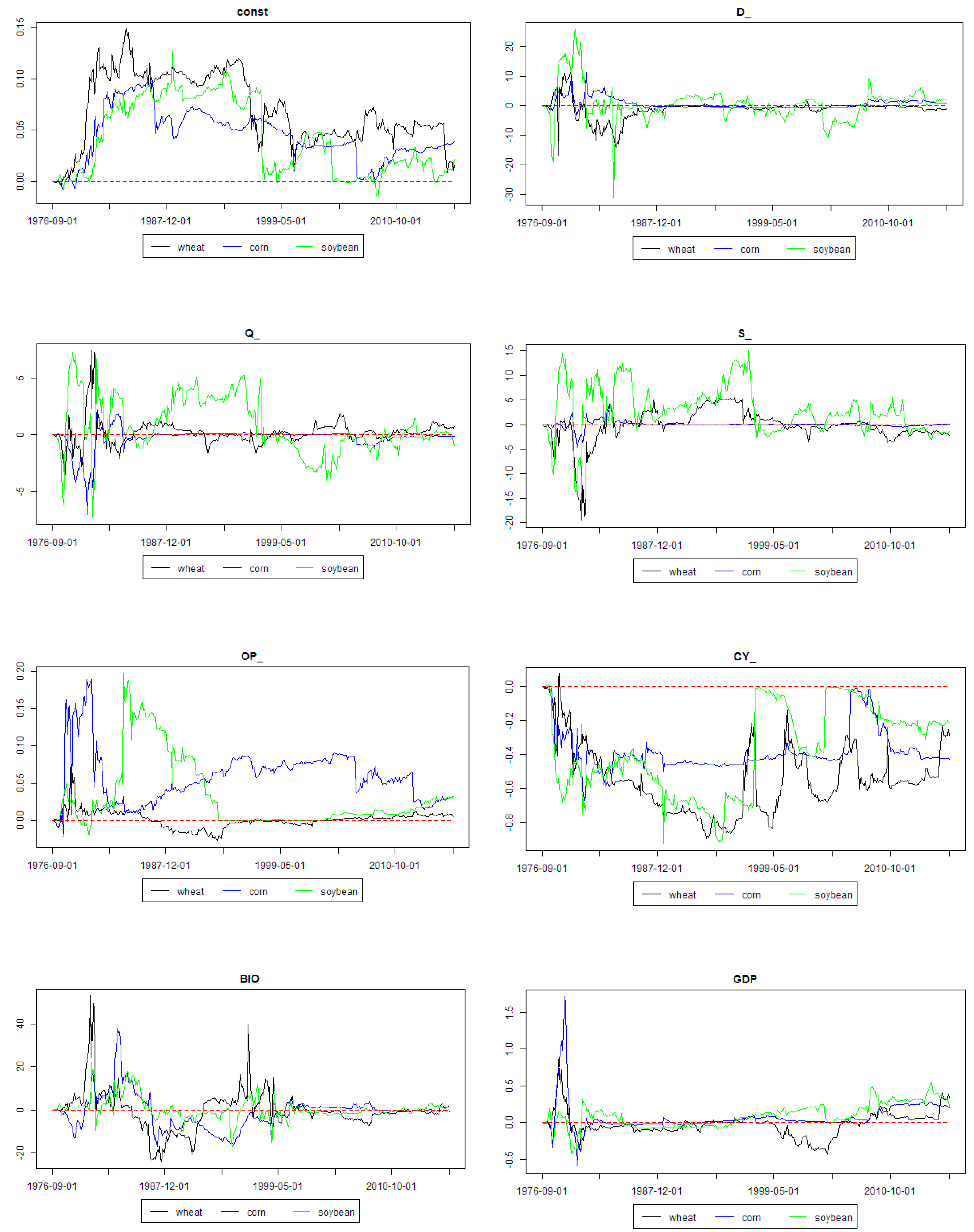
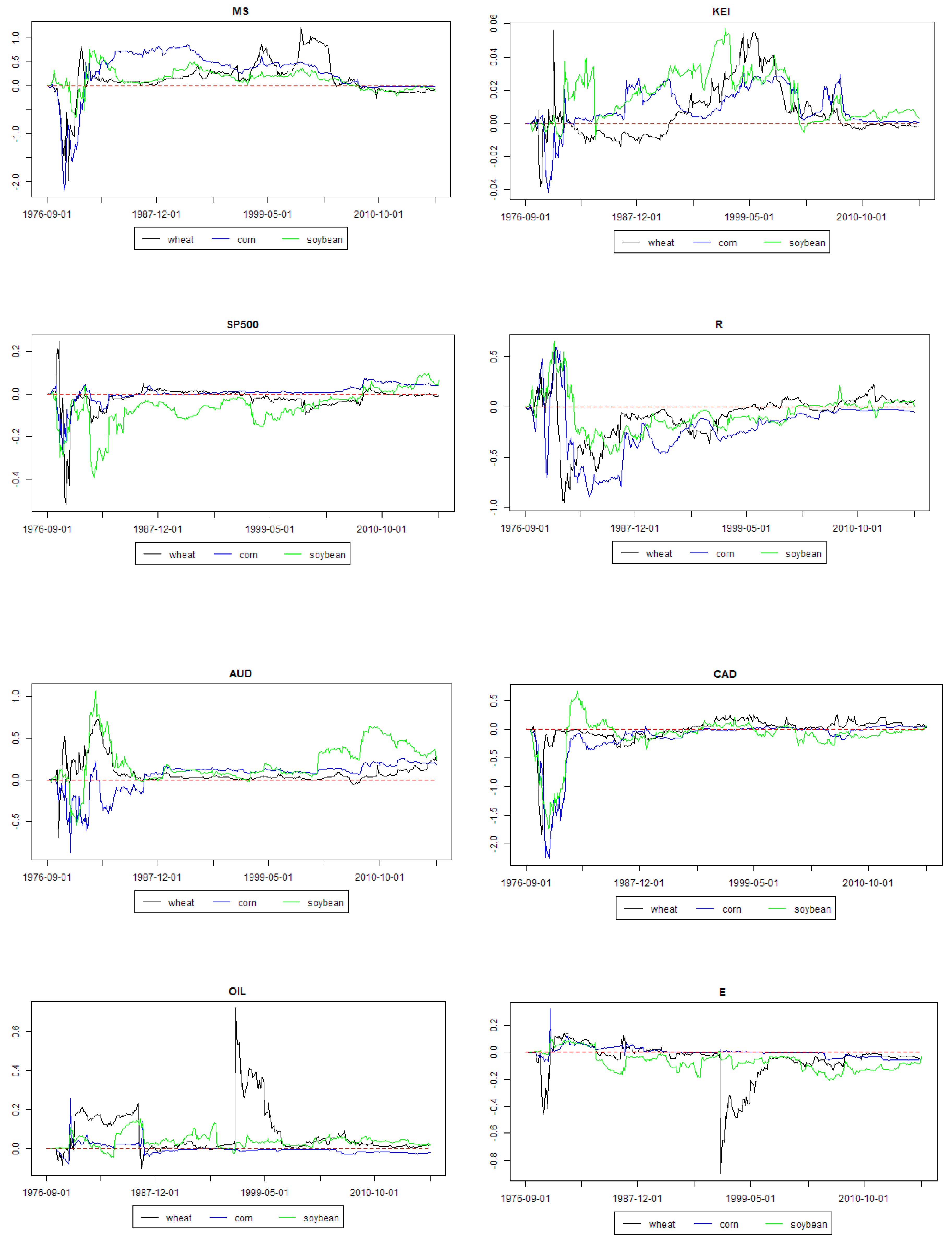
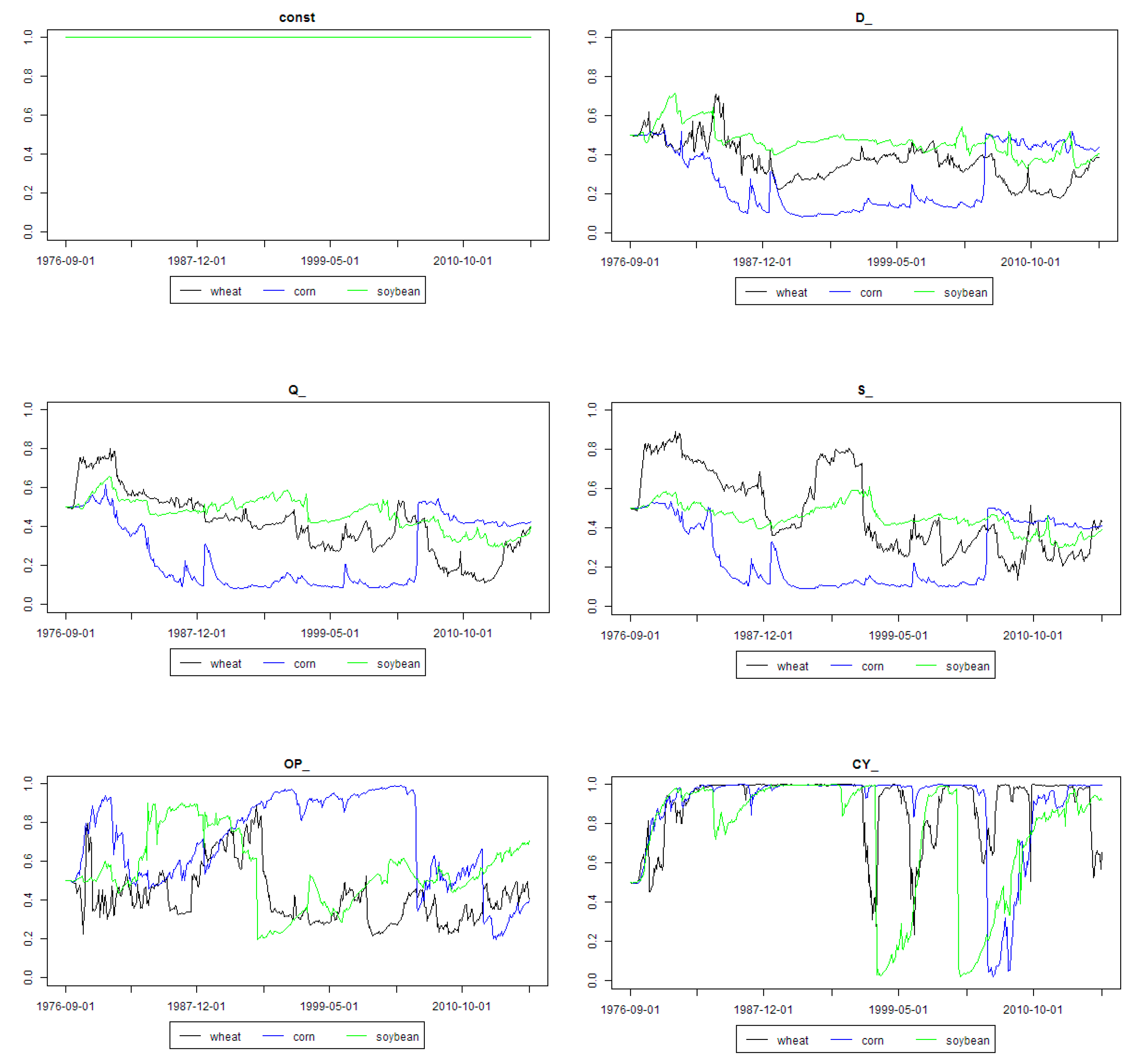
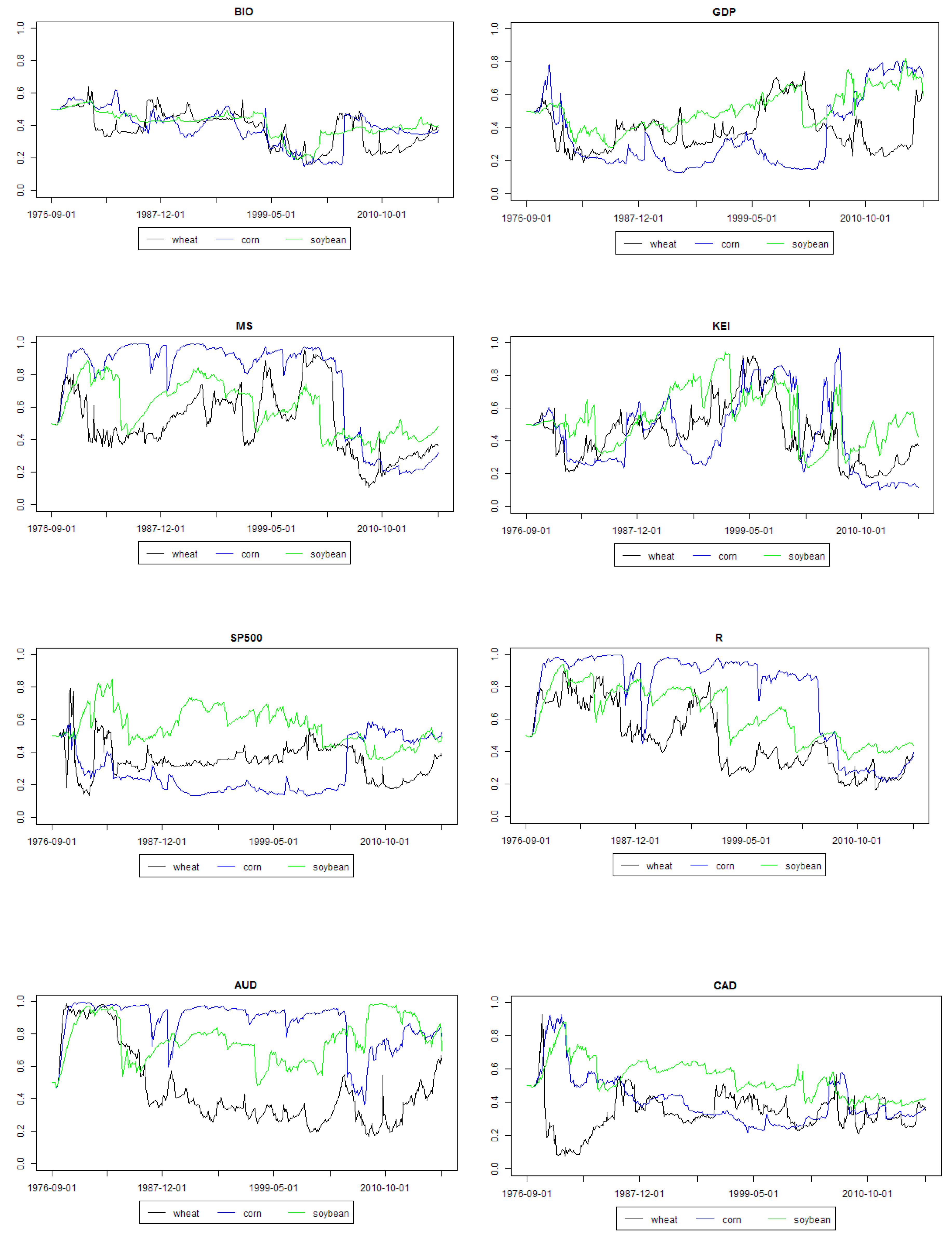
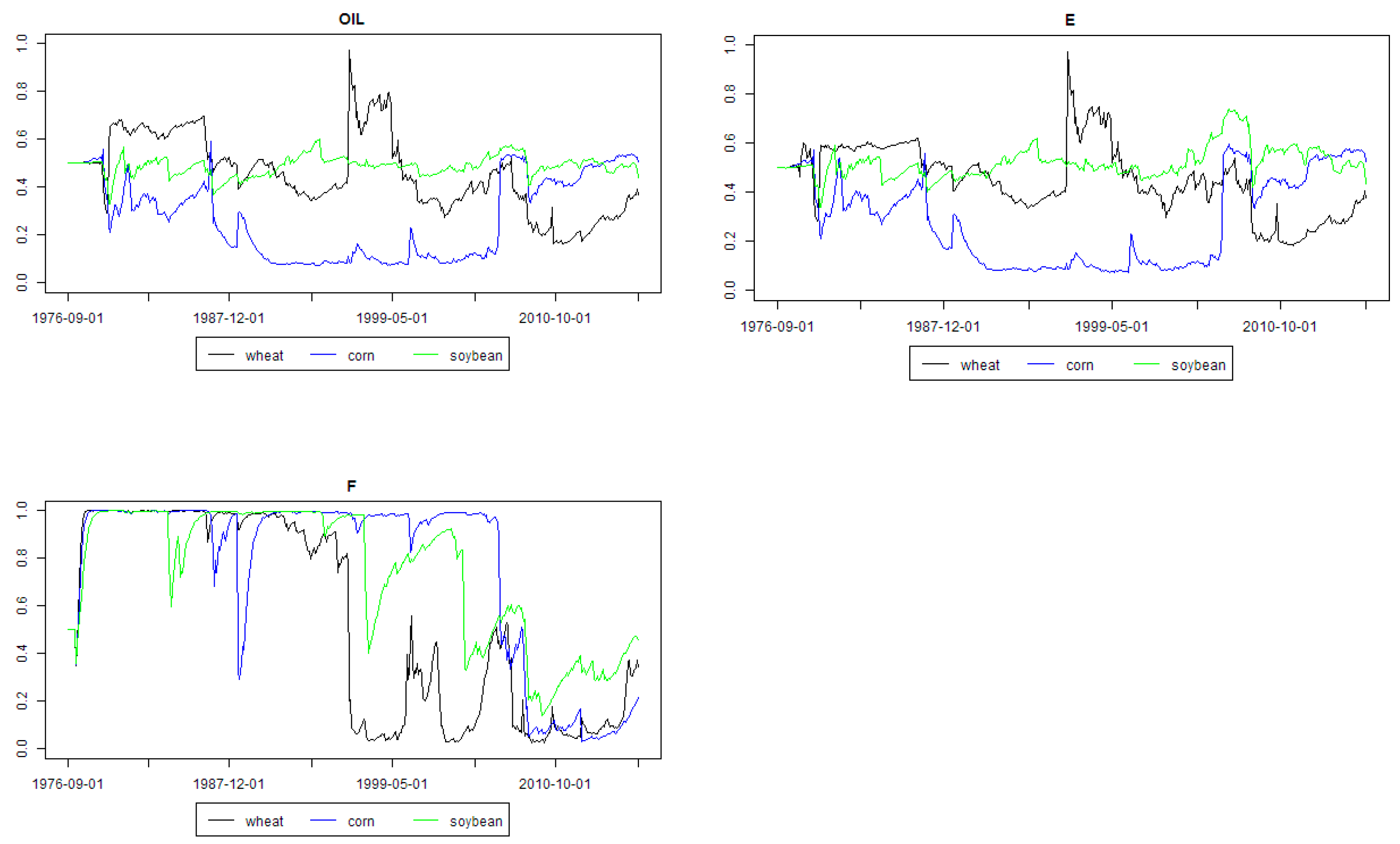
Figure 3 and Figure 4 present weighted regression coefficients and posterior inclusion probabilities for all the explanatory variables from the models minimizing MASE for the analyzed agricultural commodities. As aforementioned, these figures should be analyzed together. First of all, some first part of graphs from left (i.e., beginning period) should be considered as a period during which the model combination scheme “learns” and outcomes can be chaotic. Actually, this is the previously mentioned in-sample part of data set.

It can be seen that consumption was quite an important driver of soybean prices in the end of the 2000s. Production played an important role in the 1990s and in the beginning of the 2000s for soybean. Stock quotas played an important role for wheat and soybean in the end of the 1990s, also later there were some short periods when they played an important role as soybean price driver.

The role of open interest was important for corn between the beginning of the 1990s and end of the 2000s. Convenience yield was important driver of corn prices throughout the whole analyzed period, except the late 2000s. It was also an important driver of soybean prices in the 1990s and middle of the 2000s.

Biofuels production was an important driver for the prices of all three grain commodities in the middle of the 1990s. This result was actually a bit strange, because the corn-based biofuels growth started after the middle of 1990s. However, the sugarcane based Brazilian ethanol production had been well established even before the corn-based ethanol boom started. The role of GDP growth per capita in BRIC economies was rather marginal before 2000s, but since then it seemed to become a more and more important driver of all three grain commodities prices.

Market stress was an important driver of all three commodities prices until the middle of the 2000s. Global economic activity was an important driver of all three commodities prices in 1990s and in late 2000s. The role of stock market index was rather marginal for all the analyzed commodities throughout the whole analyzed period.

The role of interest rate decreased since the 1990s and it was marginal since the 2010s. The role of Australian dollar exchange rate increased since the 2000s, whereas the role of Canadian dollar was all the time marginal. The price of oil was an important driver of wheat price in a short period in the middle of the 1990s. A similar conclusion is valid for energy prices in the case of wheat price. However, energy prices were also quite an important driver of soybean price since the 1990s until now. Fertilizers prices were generally an important driver of all three grain commodities prices between 1990 and the middle of the 2000s, except some short periods during this time. Moreover, their role has been increasing recently.

Summarizing, it can be seen that fundamental factors (like consumption, production, stock quotas) were important price drivers, but in the past periods rather, and only for soybean. Open interest, usually considered in the context of speculative pressures, was important in the case of corn. This commodity was also influenced by convenience yield. Recently, it can be seen that the development of emerging economies is a very important price driver.

The general outlook of the results seems that fundamental factors were very important in the far past, whereas more recently the financial factors played a more important role. For the very recent period, the most important drivers were the growth of emerging economies and GDP per capita in these countries. Moreover, global economic activity, development of emerging economies, exchange rates, fertilizer prices and market stress seem to be the common price drivers for wheat, corn and soybean.

Soybean seems to be affected in certain periods quite much by fundamental factors, whereas corn by financial and speculative factors [70]. Wheat seems to be more linked with crude oil and, generally, energy prices.

It is interesting to compare the outcomes for these grain commodities with some other DMA analyses from the commodity market in general. Of course, other studies apply a completely different set of potential price drivers for other commodities, but some drivers were common. In the case of metal prices [71], it was found that supply–demand and stock quotas factors were indeed important price drivers, convenience yield was also found to be important driver, but global economic activity was found important only during short periods. Market stress and exchange rates were also found important.

If the DMA applied to crude oil price was considered, then global economic activity was also found as important driver during some periods. Similarly, exchange rates, market stress and emerging economies stock market prices [67].

It is interesting that for metals and crude oil supply–demand factors occurred to be important price drivers, whereas herein they happened not to play very important role. On the other hand, global economic activity, economic expansion of emerging economies, exchange rates and market stress seemed to be the common important price drivers for various commodities.

Finally, it should be stressed that the notion of “importance” should be considered in a relative manner [23]. In particular, it should not be understood in a sense of “absolute” manner, but rather as importance respective to the other variables considered (used) in the given model combination scheme. In other words, it can be understood that, for example, GDP growth in BRIC countries is a more important grains price driver than production, consumption, and all other factors considered in the research reported herein. Not that, for example, consumption quotas are a totally unimportant driver. Indeed, this sounds quite reasonable—the GDP growth results in increasing consumption, so it should be looked on as the most important driver, and consumption increase is its consequence. Anyway, it should be also remembered that model combination schemes are rather aimed at forecasting—not on detecting causality or explanatory relationship analysis tools [23].

As already discussed, Figure 3 and Figure 4 present averaged regression coefficients and posterior inclusion probabilities from DMA models with particular combination of forgetting factors. However, as mentioned previously, a few α and λ combinations were estimated. It can be asked, if other combinations would not result in different economic conclusions. Interestingly, the graphical analysis of plots, like in Figure 3 and Figure 4, but for all α and λ combinations used herein, indicates the same conclusions. In other words, there were some differences in case of the exact numerical values, but up to reasonably high degree the time-paths were the same. In other words, a posterior inclusion probability for the given variable increased for all considered α and λ combinations or decreased during a given period. In particular there was no situation that during some period one combination of α and λ indicated rising posterior inclusion probability for some variables, whereas some another combination—decreasing for the same variable. Similarly, this was for the averaged regression coefficients (including their signs). For clarity, the analyzed figures were not included herein. It is only mentioned, that it had been checked whether the reported economic interpretations would not depend on α and λ combinations.

6. Conclusions

The presented research was focused on applying some novel Bayesian model combination schemes to forecasting the spot prices of the selected grain commodities. First of all, it was interesting that these methods happened to produce, indeed, statistically significant more accurate one-month ahead forecasts than some conventional econometric models, like ARIMA, historical average or the naïve method. Only for soybean, it could not be said that ARIMA or NAÏVE forecasts were significantly less accurate.

It was also seen that not only the time-varying parameters approach (to regression coefficients) itself was beneficial, but also consideration of various models. In other words, combining several regression models through model averaging or model selection procedure improved forecast accuracy. Moreover, time-varying approach towards, simultaneously, both regression coefficients and model switching itself (i.e., dealing with model uncertainty) was beneficial. From the interpretative point of view it meant that the joining of these two features allowed interesting interpretation on how the importance of various grains price drivers change in time.

However, the notion of importance of a driver should be carefully understood as a relative importance, with respect to the other drivers considered in the whole forecasting scheme [23]. In other words, it should be understood rather as a factor improving forecast accuracy, not to be confused with the notion of some kind of a causal relationship. Actually, this was also some limitation of the current research. On the other hand, the performed identification of key factors influencing agricultural prices can serve as a starting point for some future research, dealing directly with studying the causal relationships.

Indeed, herein various factors were taken as potential price drivers: fundamental ones (like production, consumption, stock quotas), macroeconomic (GDP growth per capita, economic activity, etc.) and financial ones (like exchange rates, stock prices, market stress, etc.). In case of fundamental factors, they were found to be rather important ones in further periods in the past, whereas in recent years the applied econometric schemes stressed the higher role of more financial factors and, especially, GDP growth per capita in BRIC economies. This signals that the sustainable development in the studied area, and suitable policies, cannot focus solely on the production processes. They have to consider changing patterns in economies. For example, as the societies becomes richer, the consumption patterns and consumer choices can change. Secondly, links with financial instruments becomes tighter nowadays. Also, the role of derivatives becomes higher. As such, they can be used more intensively in speculation—not only for hedging purposes.

These results are in agreement with other research focusing on the role of new emerging economies, richer societies in these countries and, therefore, growing demand from these consumers. Indeed, the role of GDP growth per capita in BRIC economies was found rather marginal before the 2000s, but afterwards its role as a grain price driver started to increase. This was also an interesting point, for future considerations. In the context of the sustainable development, it can be asked whether these changes impact only the quantity of the demand, or also the quality of the product. For example, will the newly rich consumers care whether the product they buy was produced in a sustainable way [72,73,74].

The decreasing role of fundamental factors is generally in line with studies on commodities markets, indicating the rising role of, so called, financialization of commodities markets. This means that managerial decisions in the field of agriculture have to be more aware of this situation. The conventional approach based only on physical aspects, like production and distribution of the product are not enough nowadays. The market price can be impacted also by more “virtual” factors. For example, the price of an agricultural commodity can depend on both: the weather condition impacting the harvests, and general situation on financial markets—also those markets, which are not directly linked with agriculture.

Nevertheless, potential prices drivers linked with speculative pressures (like, for example, open interest) were found important only in case of corn prices in the late 2000s. However, convenience yield was found to be an important driver of corn and soybean prices in parts of the 1990s and 2000s. In recent periods, the impact of biofuels production was found rather marginal.

Stock market price index was not found as an important grain price driver. However, the index of market stress was an important driver. Overall, crude oil price, and energy prices, seemed to be important drivers of wheat prices. The financial and speculative factors seemed to be most important in case of driving corn prices, whereas fundamentals seemed to influence soybean prices the most.