Premiums for Non-Sustainable and Sustainable Components of Market Volatility: Evidence from the Korean Stock Market


Abstract
1. Introduction
2. Literature Review
3. Data and Methodology
3.1. Data
3.2. Volatilities Components
3.2.1. Volatility Decomposition
3.2.2. Factors Mimicking Volatility Components
3.3. Portfolio Analysis
3.4. Fama-MacBeth Regressions
4. Empirical Results
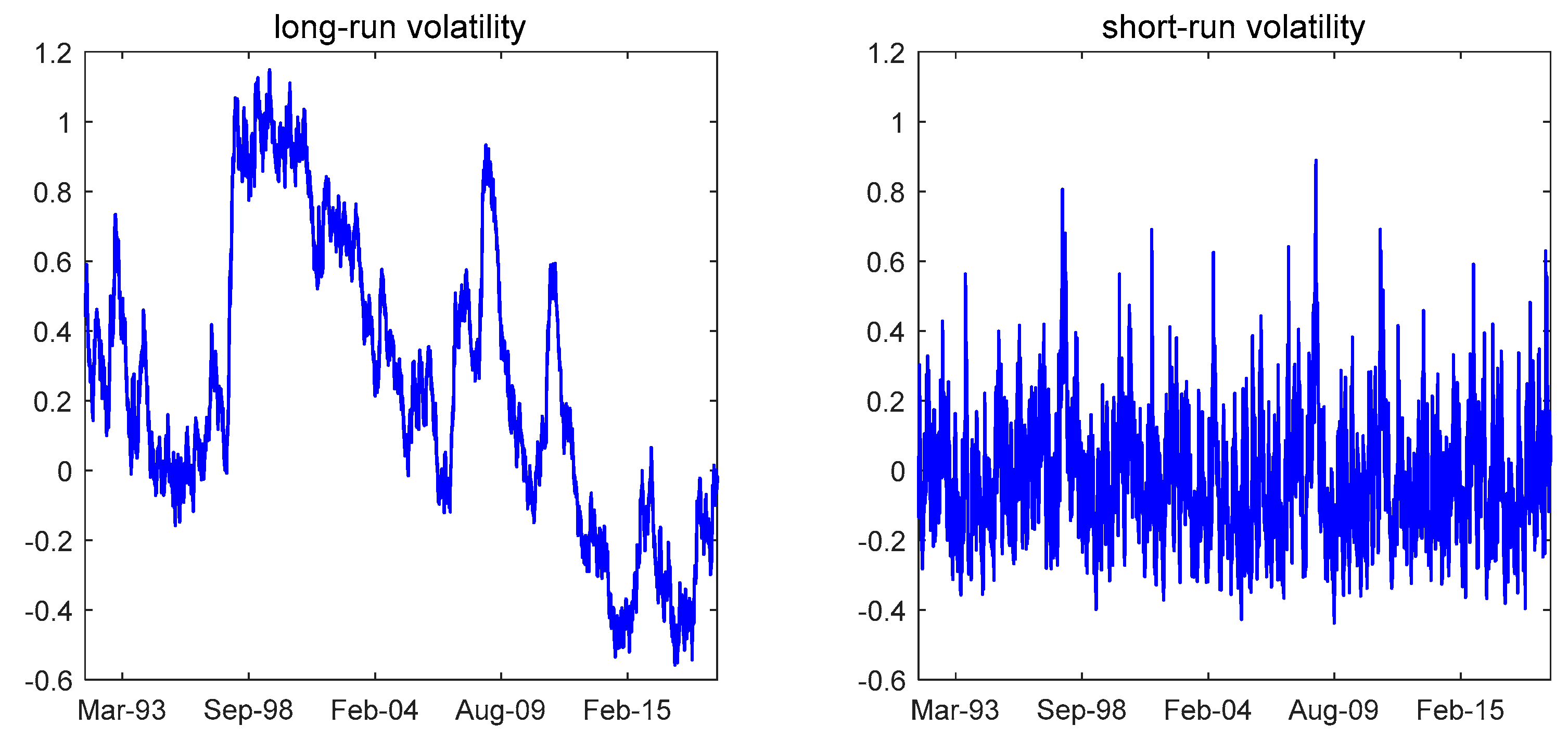
4.1. Short-and Long-Term Volatilities
4.2. Portfolio Analysis
4.3. Fama-MacBeth Regression
5. Robustness
6. Conclusions
Author Contributions
Funding
Acknowledgments
Conflicts of Interest
Appendix A
References
- Sharpe, W.F. Capital Asset Prices: A Theory of Market Equilibrium Under Conditions of Risk. J. Financ. 1964, 19, 425–442. [Google Scholar]
- Lintner, J. The Valuation of Risk Assets and the Selection of Risky Investments in Stock Portfolios and Capital Budgets. Rev. Econ. Stat. 1965, 47, 13–37. [Google Scholar] [CrossRef]
- Ang, A.; Hodrick, R.J.; Xing, Y.; Zhang, X. The Cross-Section of Volatility and Expected Returns. J. Financ. 2006, 61, 259–299. [Google Scholar] [CrossRef]
- Frazzini, A.; Pedersen, L.H. Betting against beta. J. Financ. Econ. 2014, 111, 1–25. [Google Scholar] [CrossRef]
- Engle, R.F.; Rosenberg, J.V. Testing the Volatility Term Structure Using Option Hedging Criteria. JOD 2000, 8, 10–28. [Google Scholar] [CrossRef]
- Bollerslev, T.; Zhou, H. Estimating stochastic volatility diffusion using conditional moments of integrated volatility. J. Econom. 2002, 109, 33–65. [Google Scholar] [CrossRef]
- Alizadeh, S.; Brandt, M.W.; Diebold, F.X. Range-Based Estimation of Stochastic Volatility Models. J. Financ. 2002, 57, 1047–1091. [Google Scholar] [CrossRef]
- Chacko, G.; Viceira, L.M. Spectral GMM estimation of continuous-time processes. J. Econom. 2003, 116, 259–292. [Google Scholar] [CrossRef]
- Chernov, M.; Ronald Gallant, A.; Ghysels, E.; Tauchen, G. Alternative models for stock price dynamics. J. Econom. 2003, 116, 225–257. [Google Scholar] [CrossRef]
- Maheu, J. Can GARCH Models Capture Long-Range Dependence? Stud. Nonlinear Dyn. Econom. 2005, 9. [Google Scholar] [CrossRef]
- Brandt, M.W.; Jones, C.S. Volatility Forecasting With Range-Based EGARCH Models. J. Bus. Econ. Stat. 2006, 24, 470–486. [Google Scholar] [CrossRef]
- Speight, A.E.H.; McMillan, D.G.; Gwilym, O. ap Intra-day volatility components in FTSE-100 stock index futures. J. Futures Mark. 2000, 20, 425–444. [Google Scholar] [CrossRef]
- Christoffersen, P.; Jacobs, K.; Ornthanalai, C.; Wang, Y. Option valuation with long-run and short-run volatility components☆. J. Financ. Econ. 2008, 90, 272–297. [Google Scholar] [CrossRef]
- Ané, T. Short and long term components of volatility in Hong Kong stock returns. Appl. Financ. Econ. 2006, 16, 439–460. [Google Scholar] [CrossRef]
- Adrian, T.; Rosenberg, J. Stock returns and volatility: Pricing the short-run and long-run components of market risk. J. Financ. 2008, 63, 2997–3030. [Google Scholar] [CrossRef]
- Yang, Y.; Copeland, L. The cross-sectional risk premium of decomposed market volatility in UK stock market. Open J. Soc. Sci. 2014, 2, 30. [Google Scholar] [CrossRef][Green Version]
- Guo, H.; Neely, C.J. Investigating the intertemporal risk–return relation in international stock markets with the component GARCH model. Econ. Lett. 2008, 99, 371–374. [Google Scholar] [CrossRef]
- Zhu, J. Pricing volatility of stock returns with volatile and persistent components. Financ. Mark. Portf. Manag. 2009, 23, 243–269. [Google Scholar] [CrossRef]
- Park, S.; Jung, H. The Effect of Managerial Ability on Future Stock Price Crash Risk: Evidence from Korea. Sustainability 2017, 9, 2334. [Google Scholar] [CrossRef]
- Merton, R.C. An intertemporal capital asset pricing model. Econom. J. Econom. Soc. 1973, 867–887. [Google Scholar] [CrossRef]
- Fama, E.F.; MacBeth, J.D. Risk, Return, and Equilibrium: Empirical Tests. J. Political Econ. 1973, 81, 607–636. [Google Scholar] [CrossRef]
- Fama, E.F.; French, K.R. Common risk factors in the returns on stocks and bonds. J. Financ. Econ. 1993, 33, 3–56. [Google Scholar] [CrossRef]
- Altman, E.I.; Schwartz, R.A. Common Stock Price Volatility Measures and Patterns. J. Financ. Quant. Anal. 1970, 4, 603–625. [Google Scholar] [CrossRef]
- Pinches, G.E.; Kinney, W.R. The measurement of the volatility of common stock prices. J. Financ. 1971, 26, 119–125. [Google Scholar] [CrossRef]
- Black, F.; Scholes, M. The Pricing of Options and Corporate Liabilities. J. Political Econ. 1973, 81, 637–654. [Google Scholar] [CrossRef]
- Merton, R.C. Theory of Rational Option Pricing. Bell J. Econ. Manag. Sci. 1973, 4, 141. [Google Scholar] [CrossRef]
- French, K.R.; Schwert, G.W.; Stambaugh, R.F. Expected stock returns and volatility. J. Financ. Econ. 1987, 19, 3–29. [Google Scholar] [CrossRef]
- Engle, R.F.; Lilien, D.M.; Robins, R.P. Estimating Time Varying Risk Premia in the Term Structure: The Arch-M Model. Econometrica 1987, 55, 391. [Google Scholar] [CrossRef]
- Goyal, A.; Saretto, A. Cross-section of option returns and volatility. J. Financ. Econ. 2009, 94, 310–326. [Google Scholar] [CrossRef]
- Chou, R.Y. Volatility persistence and stock valuations: Some empirical evidence using garch. J. Appl. Econ. 1988, 3, 279–294. [Google Scholar] [CrossRef]
- Campbell, J.Y.; Hentschel, L. No news is good news. J. Financ. Econ. 1992, 31, 281–318. [Google Scholar] [CrossRef]
- Ghysels, E.; Santa-Clara, P.; Valkanov, R. There is a risk-return trade-off after all. J. Financ. Econ. 2005, 76, 509–548. [Google Scholar] [CrossRef]
- Guo, H.; Whitelaw, R.F. Uncovering the Risk-Return Relation in the Stock Market. J. Financ. 2006, 61, 1433–1463. [Google Scholar] [CrossRef]
- Sehgal, S.; Garg, V.; Deisting, F. Relationship between cross sectional volatility and stock returns: Evidence from India. Invest. Manag. Financ. Innov. 2012, 9, 91–100. [Google Scholar]
- Breen, W.; Glosten, L.R.; Jagannathan, R. Economic Significance of Predictable Variations in Stock Index Returns. J. Financ. 1989, 44, 1177–1189. [Google Scholar] [CrossRef]
- Turner, C.M.; Startz, R.; Nelson, C.R. A Markov model of heteroskedasticity, risk, and learning in the stock market. J. Financ. Econ. 1989, 25, 3–22. [Google Scholar] [CrossRef]
- Baillie, R.T.; DeGennaro, R.P. Stock Returns and Volatility. J. Financ. Quant. Anal. 1990, 25, 203. [Google Scholar] [CrossRef]
- Chou, R.; Engle, R.F.; Kane, A. Measuring risk aversion from excess returns on a stock index. J. Econom. 1992, 52, 201–224. [Google Scholar] [CrossRef]
- Glosten, L.R.; Jagannathan, R.; Runkle, D.E. On the Relation between the Expected Value and the Volatility of the Nominal Excess Return on Stocks. J. Financ. 1993, 48, 1779–1801. [Google Scholar] [CrossRef]
- Da, Z.; Schaumburg, E. The Pricing of Volatility Risk Across Asset Classes; Unpublished Working Paper; University of Notre Dame: Notre Dame, IN, USA; Federal Reserve Bank of New York: New York, NY, USA, 2011. [Google Scholar]
- Cremers, M.; Halling, M.; Weinbaum, D. Aggregate jump and volatility risk in the cross-section of stock returns. J. Financ. 2015, 70, 577–614. [Google Scholar] [CrossRef]
- Sehgal, S.; Garg, V. Cross-sectional Volatility and Stock Returns: Evidence for Emerging Markets. Vikalpa 2016, 41, 234–246. [Google Scholar] [CrossRef]
- Dimitriou, D.; Simos, T. The relationship between stock returns and volatility in the seventeen largest international stock markets: A semi-parametric approach. Mod. Econ. 2011, 1, 1–8. [Google Scholar] [CrossRef]
- Lee, C.F.; Chen, G.; Rui, O.M. Stock Returns and Volatility on China’s Stock Markets. J. Financ. Res. 2001, 24, 523–543. [Google Scholar] [CrossRef]
- De Santis, G.; Imrohoroǧlu, S. Stock returns and volatility in emerging financial markets. J. Int. Money Financ. 1997, 16, 561–579. [Google Scholar] [CrossRef]
- Shin, J. Stock returns and volatility in emerging stock markets. Int. J. Bus. Econ. 2005, 4, 31–43. [Google Scholar]
- Chiang, T.C.; Doong, S.-C. Empirical Analysis of Stock Returns and Volatility: Evidence from Seven Asian Stock Markets Based on TAR-GARCH Model. Rev. Quant. Financ. Account. 2001, 17, 301–318. [Google Scholar] [CrossRef]
- Xu, X.; Taylor, S.J. The Term Structure of Volatility Implied by Foreign Exchange Options. J. Financ. Quant. Anal. 1994, 29, 57–74. [Google Scholar] [CrossRef]
- Bates, D.S. Post-’87 crash fears in the S&P 500 futures option market. J. Econom. 2000, 94, 181–238. [Google Scholar]
- Newey, W.K.; West, K.D. A Simple, Positive Semi-Definite, Heteroskedasticity and Autocorrelation Consistent Covariance Matrix. Econometrica 1987, 55, 703–708. [Google Scholar] [CrossRef]
- Campbell, J.Y. Understanding risk and return. J. Political Econ. 1996, 104, 298–345. [Google Scholar] [CrossRef]
- Chen, J.S. Intertemporal CAPM and the Cross-Section of Stock Returns; Unpublished Working Paper; University of Southern California: Los Angeles, CA, USA, 2003. [Google Scholar]
- Bakshi, G.; Kapadia, N. Volatility Risk Premiums Embedded in Individual Equity Options. J. Deriv. 2003, 11, 45. [Google Scholar] [CrossRef]
- Nelson, D.B. Conditional Heteroskedasticity in Asset Returns: A New Approach. Econometrica 1991, 59, 347–370. [Google Scholar] [CrossRef]


| 0.0106 | −0.0813 | 0.0115 | 0.9339 | −0.0450 | 0.0600 | 0.0011 | 0.9989 | −0.0027 | 0.0298 |
| (0.0147) | (0.0724) | (0.0358) | (0.0092) | (0.0040) | (0.0064) | (0.0003) | (0.0004) | (0.0020) | (0.0034) |
| Flres | Fsres | MKT | SMB | HML | |
|---|---|---|---|---|---|
| Min | −0.544 | −1.006 | −24.466 | −20.372 | −19.306 |
| Max | 0.770 | 1.739 | 41.952 | 37.037 | 21.977 |
| Mean | 0.011 | 0.032 | 0.348 | 0.430 | 0.786 |
| Std. Dev | 0.156 | 0.302 | 7.537 | 5.935 | 4.503 |
| Skewness | 0.923 | 0.669 | 0.678 | 0.521 | 0.041 |
| Kurtosis | 4.667 | 3.669 | 3.595 | 4.711 | 4.356 |
| Panel A: Sorted on Flres | Panel B: Sorted on Fsres | ||||
|---|---|---|---|---|---|
| Portfolio | Return (%) | Flres | Portfolio | Return (%) | Fsres |
| 1—Low | 32.78 | −53.85 | 1—Low | 32.75 | −27.38 |
| (4.08) | (−8.14) | (4.08) | (−11.99) | ||
| 2 | 11.37 | −15.4 | 2 | 11.39 | −8.56 |
| (2.17) | (−5.96) | (2.15) | (−7.27) | ||
| 3 | 5.61 | 2.76 | 3 | 5.68 | 0.33 |
| (1.25) | (1.96) | (1.19) | (0.33) | ||
| 4 | 5.42 | 20.39 | 4 | 5.22 | 9.20 |
| (1.14) | (9.45) | (1.10) | (6.53) | ||
| 5—High | 18.78 | 57.68 | 5—High | 18.90 | 28.17 |
| (2.98) | (11.61) | (3.26) | (10.54) | ||
| High-low | −14.00 ** | 111.53 *** | High-low | −13.85 *** | 55.56 *** |
| (−2.52) | (10.21) | (−2.61) | (13.65) | ||
| Panel A: Regression with 25 Portfolios | ||||||||
|---|---|---|---|---|---|---|---|---|
| Equal-Weight | Value-Weight | |||||||
| Model | I | II | III | IV | I | II | III | IV |
| Intercept | 12.298 ** | 13.651 ** | 11.102 ** | −0.899 | 2.451 | 4.336 | 3.571 | −1.973 |
| (2.34) | (2.27) | (2.26) | (−0.19) | (0.55) | (0.84) | (0.85) | (−0.46) | |
| MKT | 1.947 | −2.817 | 0.578 | 7.496 | 8.917 ** | 4.89 | 6.378 * | 8.396 |
| (0.37) | (−0.59) | (0.11) | (1.23) | (2.04) | (1.32) | (1.67) | (1.53) | |
| Flres | −0.500 *** | −0.373 *** | −0.315 *** | −0.362 *** | −0.308 *** | −0.287 *** | ||
| (−3.01) | (−2.74) | (−3.02) | (−2.85) | (−2.80) | (-3.96) | |||
| Fsres | −0.468 * | −0.467 * | −0.556 ** | −0.500 ** | −0.521 ** | −0.601 *** | ||
| (−1.65) | (−1.86) | (-2.32) | (−2.22) | (−2.34) | (−2.62) | |||
| HML | 11.711 *** | 9.025 *** | ||||||
| (3.30) | (2.87) | |||||||
| SMB | 10.079 *** | 4.761 | ||||||
| (2.61) | (1.63) | |||||||
| Adj. R2 | 0.271 *** | 0.251 *** | 0.344 *** | 0.498 *** | 0.258 *** | 0.233 *** | 0.314 *** | 0.442 *** |
| (8.18) | (7.41) | (9.77) | (15.52) | (8.12) | (6.60) | (9.05) | (14.22) | |
| Panel B: Regression with Individual Stocks | ||||||||
| Model | I | II | III | IV | ||||
| Intercept | 8.635 ** | 7.860 * | 7.758 ** | 3.557 | ||||
| (2.16) | (1.96) | (1.98) | (1.02) | |||||
| MKT | 7.611 ** | 7.202 ** | 7.740 ** | 8.473 ** | ||||
| (2.32) | (2.52) | (2.39) | (2.37) | |||||
| Flres | −0.125 ** | −0.111 ** | −0.095 * | |||||
| (−2.10) | (−2.02) | (−1.75) | ||||||
| Fsres | −0.361 *** | −0.340 *** | −0.332 *** | |||||
| (−3.10) | (−3.04) | (−3.07) | ||||||
| HML | 2.305 | |||||||
| (1.65) | ||||||||
| SMB | 3.853 ** | |||||||
| (2.26) | ||||||||
| Adj.R2 | 0.065 *** | 0.065 *** | 0.083 *** | 0.109 *** | ||||
| (5.23) | (4.55) | (5.44) | (6.23) | |||||
| Panel A: Sorted on Flres | Panel B: Sorted on Fsres | ||||
|---|---|---|---|---|---|
| Portfolio | Return | Flres | Portfolio | Return | Fsres |
| 1—Low | 26.61 | −44.39 | 1—Low | 28.13 | −22.12 |
| (4.50) | (−11.05) | (4.34) | (−12.82) | ||
| 2 | 10.11 | −13.35 | 2 | 10.72 | −7.71 |
| (2.00) | (−6.93) | (2.01) | (−8.21) | ||
| 3 | 6.66 | 1.41 | 3 | 6.61 | −1.05 |
| (1.36) | (0.95) | (1.36) | (−1.58) | ||
| 4 | 7.39 | 16.07 | 4 | 7.48 | 5.40 |
| (1.40) | (9.31) | (1.55) | (8.54) | ||
| 5—High | 19.49 | 47.09 | 5—High | 17.31 | 19.02 |
| (3.22) | (14.29) | (3.10) | (19.93) | ||
| High-low | −7.12 ** | 91.48 *** | High-low | −10.82 *** | 41.14 *** |
| (−2.19) | (14.13) | (−3.43) | (18.96) | ||
| Panel A: Regression with 25 Portfolios | ||||||||
|---|---|---|---|---|---|---|---|---|
| Equal-Weight | Value-Weight | |||||||
| Model | I | II | III | IV | I | II | III | IV |
| Intercept | 6.912 | 5.969 | 3.768 | −3.824 | 0.735 | 0.812 | 1.298 | −3.186 |
| (1.47) | (1.23) | (0.81) | (−0.90) | (0.15) | (0.16) | (0.27) | (−0.81) | |
| MKT | 2.938 | 3.107 | 4.184 | 8.529 * | 9.573 *** | 8.012 ** | 7.641 ** | 9.796 ** |
| (0.66) | (0.73) | (0.97) | (1.84) | (2.65) | (2.34) | (2.24) | (2.24) | |
| Flres | −0.300 ** | −0.286 ** | −0.280 *** | −0.283 *** | −0.274 *** | −0.207 *** | ||
| (−2.01) | (−2.38) | (−2.78) | (−2.64) | (−2.95) | (−2.64) | |||
| Fsres | −0.777 ** | −0.730 ** | −0.561 ** | −0.625 ** | −0.582 ** | −0.425 ** | ||
| (−2.29) | (−2.18) | (−2.14) | (−2.49) | (−2.41) | (−2.36) | |||
| HML | 11.978 *** | 7.853 *** | ||||||
| (3.44) | (2.76) | |||||||
| SMB | 8.845 *** | 4.222 | ||||||
| (2.74) | (1.46) | |||||||
| Adj. R2 | 0.177 *** | 0.219 *** | 0.249 *** | 0.400 *** | 0.160 *** | 0.174 *** | 0.214 *** | 0.355 *** |
| (6.03) | (7.17) | (7.71) | (12.11) | (5.38) | (5.28) | (6.26) | (9.75) | |
| Panel B: Regression with Individual Stocks | ||||||||
| Model | I | II | III | IV | ||||
| Intercept | 7.154 * | 6.573 | 6.485 | 1.242 | ||||
| (1.75) | (1.62) | (1.62) | (0.36) | |||||
| MKT | 7.935 *** | 7.825 *** | 8.167 *** | 9.078 *** | ||||
| (2.97) | (3.09) | (3.02) | (2.79) | |||||
| Flres | −0.136 ** | −0.121 ** | −0.109 * | |||||
| (−2.21) | (−2.10) | (−1.86) | ||||||
| Fsres | −0.358 *** | −0.351 *** | −0.361 *** | |||||
| (−3.33) | (−3.38) | (−3.40) | ||||||
| HML | 3.474 ** | |||||||
| (2.35) | ||||||||
| SMB | 4.140 ** | |||||||
| (2.34) | ||||||||
| Adj. R2 | 0.069 *** | 0.071 *** | 0.092 *** | 0.128 *** | ||||
| (6.24) | (5.27) | (6.71) | (8.45) | |||||
© 2019 by the authors. Licensee MDPI, Basel, Switzerland. This article is an open access article distributed under the terms and conditions of the Creative Commons Attribution (CC BY) license (http://creativecommons.org/licenses/by/4.0/).
Share and Cite
Truong, T.T.T.; Kim, J. Premiums for Non-Sustainable and Sustainable Components of Market Volatility: Evidence from the Korean Stock Market. Sustainability 2019, 11, 5123. https://doi.org/10.3390/su11185123
Truong TTT, Kim J. Premiums for Non-Sustainable and Sustainable Components of Market Volatility: Evidence from the Korean Stock Market. Sustainability. 2019; 11(18):5123. https://doi.org/10.3390/su11185123
Chicago/Turabian StyleTruong, Thuy Thi Thu, and Jungmu Kim. 2019. "Premiums for Non-Sustainable and Sustainable Components of Market Volatility: Evidence from the Korean Stock Market" Sustainability 11, no. 18: 5123. https://doi.org/10.3390/su11185123
APA StyleTruong, T. T. T., & Kim, J. (2019). Premiums for Non-Sustainable and Sustainable Components of Market Volatility: Evidence from the Korean Stock Market. Sustainability, 11(18), 5123. https://doi.org/10.3390/su11185123