Government Regulations on Closed-Loop Supply Chain with Evolutionarily Stable Strategy

Abstract

The government plays a critical role in the promotion of recycling strategy among supply chain members. The purpose of this study is to investigate the optimal government policies on closed-loop supply chains and how these policies impact the market demand and the returning strategies of manufacturers and retailers. This paper presents a design of closed-loop supply chains under government regulation by considering a novel three-stage game theoretic model. Firstly, Stackelberg models are adopted to describe the one-shot game between the manufacturer and the retailer in a local market. Secondly, based on the Stackelberg equilibriums, a repeated and dynamic population game is developed. Thirdly, the government analyzes the population game to find the optimal tax and subsidy policies in the whole market. To solve the proposed model, the idea of backward induction is adopted. The results suggest that, by collecting tax and allocating subsidy, the government can influence the market demands and return rates. The centralized supply chain structure is always preferred for the government and the market. The government prefers to allocate subsidy to low-pollution, low-profit remanufactured products. The environmental attention of the government affects the subsidy policy.

1. Introduction

In recent years, the importance of environmental protection has been recognized. Used products may cause various environmental issues. However, through remanufacturing, the residual values of used products can bring economic benefits. For example, used products such as auto and home appliances contain a large amount of recyclable metal, plastics, and other resources. By recycling those products, the resources can be effectively reused to promote the sustainability of a society. Also, new products are more environment-friendly than old products. For example, compared with ordinary vehicles, electric vehicles use clean energy and are more energy-efficient.

A new concept, the closed-loop supply chain, has been proposed to enhance collecting and remanufacturing. Different from the typical supply chain that only focuses on the forward direction, a closed-loop supply chain consists of both forward and backward activities which involve the movement of used products from customers to upstream suppliers and improves economic and environmental performance [1,2]. Therefore, it is important to promote closed-loop supply and remanufacturing processes for both firms and governments.

The government plays a vital role in the promotion and operation of closed-loop supply chains [3]. In a closed-loop supply chain under government regulation, the firms’ decisions are unavoidably influenced by the government’s policies. For example, when the government allocates subsidies to the remanufactured products produced by the manufacturers. Subsidy level will directly affect the manufacturing costs, and moreover the wholesale price, retail price, and the return rate indirectly. Similarly, the firm’s price policy and remanufacture policy are also influenced by the tax policy of the government. Also, the government’s policy is normally a long-term decision. For those reasons, it is very important for the government to make the “right decision”.

In practical, governments have many measures to promote closed-loop supply chains. To spur domestic consumption, curb pollution and save resources, China has implemented the “old-for-new” policy for auto and home appliance replacements. In 2009, the “old-for-new” started from Beijing, Shanghai and other 7 cities as a pilot program. Customers receive 10% of the sale price as a subsidy on five kinds of new appliances including TV sets, refrigerators, washing machines, air-conditioners and computers [3,4]. By the end of 2011, the program received around 84 million units of used home appliances and recycled about 97 tons of steel, non-ferrous metal, and other resources. In January 2019, China announced an implementation guidance which indicates that green products and home appliance replacements will still be supported with an appropriate subsidy.

In Japan, a series of laws have been enacted to promote the recycling of end-of-life vehicles (ELVs), construction material, home appliances, etc. The home appliance recycling law was enacted in June 1998 and was enforced in April 2001; this law detailed stipulates the obligations of each player in the recycling process [5]. Consumers need to pay for collection and recycling. The retailers collect the used appliances and transfer them to a designated collection site. Then, the manufacturers collect the used appliances from the collection site and take charge of recycling. In this process, the obligations of the government are to provide necessary information on recycling and to impose a penalty on the business entities that make improper claims.

In this paper, we consider the government as the Stackelberg leader. A Stackelberg competition model-based optimization model is designed to find the best tax and subsidy policies for the government. By using evolutionary game theory, we develop a repeated and dynamic population game which consists of multiple manufacturers and retailers, so that the government can observe the whole market to make long-term decisions. Also, in each local market, the Stackelberg competition model is considered between a manufacturer and a retailer to find the optimal price policy and return policy, while the manufacturer is the supply chain leader and the retailer is the follower. The supply chain model considered in this paper consists of a government and a supply chain consisting of multiple manufacturers which remanufacture used products and multiple retailers in multiple local markets. The proposed model includes one government, multiple manufacturers and retailers. Based on the proposed model, the following questions are mainly discussed:

• What are the best tax and subsidy policies when the government faces different scenarios and how do the government regulations influence the wholesale price, retail price and the return rate?
• Which closed-loop supply chain structure is preferred for the government and will the structure be selected by the market?
• What kind of products are worth allocating a high subsidy to?

By analyzing existing studies, we conclude that prior research has mainly focused on the influence of government subsidy policy on the behavior of a few firms. To find the best subsidy policy for the government considering environmental impacts and public revenue, and influences of the policies in the whole market that includes the population dynamics of manufacturers and retailers, are still open questions.

To address those gaps, in this paper, a government optimization model is proposed to decide the optimal tax and subsidy policies in a closed-loop supply chain. The government model is based on the results of an evolutionary game analysis that allows us to analyze how the policy influences the whole market. Also, the closed-form Stackelberg equilibriums of the basic models are solved, so that we can develop the evolutionary game. Finally, numerical experiments are conducted to illustrate the selected policies when the government faces different scenarios.

The rest of this paper is organized as follows. Section 2 reviews relevant literature. Section 3 presents the proposed game models which include one-shot Stackelberg competition models between the manufacturer and the retailer, evolutionary game model and a Stackelberg competition-based government optimization model. Numerical experiments in different scenarios are conducted in Section 4. Finally, the conclusions are summarized in Section 5.

2. Literature Review

2.1. Closed-Loop Supply Chain Design Problem

Channel design is one of the important research streams in closed-loop supply chains [6]. Stackelberg competition models are widely used to describe the relationship between manufacturers and retailers [7,8,9,10,11,12,13,14,15,16]. Savaskan et al. (2004) [7] studied the problem of choosing the appropriate closed-loop supply chain structure for collecting the used products. To address this problem, a two-echelon supply chain that includes a manufacturer and a retailer was considered. In the supply chain, the used products can be collected by the manufacturer, or the retailer, or the third-party. Using a Stackelberg model, the optimal wholesale price, retail price and product return rate of the manufacturer and the retailer were obtained. They found that the retailer collection was the most effective supply chain structure for the manufacturer. In the same way, Savaskan and Van Wassenhove (2006) [8] extended Savaskan et al.’s (2004) [7] work to a competitive retailing environment. In their paper, a supply chain that includes two competing retailers was considered. The manufacturer can either directly collect the used products form the customers, or indirectly collect via retailers. Continually, De Giovanni and Zaccour (2014) [9] extended Savaskan el al.’s (2004) [7] work from single-period to a two-period closed-loop supply chain model, in which a part of the new products that sold in the first period are recycled from the customers in the second period. Based on the two-period model, Genc and De Giovanni (2017) [17] and Xu and Wang (2018) [10] developed closed-loop supply chain models considering technology level and emission reduction, respectively. Sarkar et al. (2017) [18] examined the impacts of carbon emission from production and transportation in a closed-loop supply chain which adopts returnable transport items for transportation. Sarkar et al. (2019) [19] developed a multi-objective model to minimize carbon emissions and maximize total profit in a closed-loop supply chain. In their model, a self-healing polymer-based returnable transport packing is considered in reverse logistics.

The similar closed-loop supply chain structurers in Savaskan et al.’s (2004) [7] paper are adopted in this paper. Our model is an extension of Savaskan et al.’s (2004) [7] work by considering the dynamic process, government regulation and multiple manufacturers and retailers.

Different from the former studies, we investigate the closed-loop supply chain design problem from both the government’s perspective and the market’s perspective. The structure that the government preferred and the structure that the market selected are respectively illustrated in the current study. Moreover, by adopting an evolutionary game model, a multi-period closed-loop supply chain model is considered.

2.2. Closed-Loop Supply Chain with Government Tax and Subsidy

The government plays an important role in the closed-loop supply chain. Ma et al. (2013) [3] studied the influence of the government consumption-subsidy program on a closed-loop supply chain, in which the manufacturer produces new products and one retailer and one e-retailer sell the products to the consumers. They found that all the consumers could benefit from the government consumption-subsidy program. Xiong et al. (2013) [20] considered a closed-loop supply chain that consists of a supplier and a manufacturer. They illustrated that remanufacturing was beneficial to the environment when the government allocates subsidy to the integrated manufacturer. Wang et al. (2014) [21] addressed the channel design problem for the remanufacturer who can either sell the remanufactured products to the customers via the manufacturer or directly sell to the customers. They found that the subsidy can promote remanufacturing activities. Wang et al. (2017) [22] examined a reward-penalty mechanism in a closed-loop supply chain that includes two sequential competing manufacturers and one retailer. They assumed that the government can implement the reward-penalty mechanism to the closed-loop supply chain. By calculating the equilibrium solutions, the supply chains with or without government regulation were both investigated. Saha et al. (2016) [23] analyzed a reward-driven policy in a closed-loop supply chain. The pricing and remanufacturing strategies are obtained in both the non-cooperative and centralized model.

Recently, Nielsen et al. (2019) [24] investigated two government incentive policies in a green supply chain. One policy is that the government provides incentives on the R&D investment, and the other policy is that the government offers incentives on the unit product. The social welfare function is concave with respect to government incentive rates in this model. Wan and Hong (2019) [25] examined the effects of transfer pricing policies and subsidy policies in a closed-loop supply chain. Two recyclers, one retailer and one third-party, are considered in their model. He et al. (2019) [26] obtained the best channel structure and pricing strategies for the manufacturer and the optimal subsidy policies for the government. Their supply chain model consists of one manufacturer, one retailer and one third-party.

Most of the literature focused on the influence of government regulation on several manufacturers and retailers. In this paper, we analyze the government’s influences on the whole market that includes multiple manufacturers and retailers by developing the dynamic population game via evolutionary game theory.

2.3. Evolutionary Game Theory in Supply Chains

Li et al. (2014) [27] developed an evolutionary game model with a two-echelon closed-loop supply chain to study evolutionarily stable strategies (ESS) of manufacturers and retailers. They found that pricing is an important factor to determine the evolutionarily stable strategies and government subsidy can support the growth of the remanufacturing industry. Ji et al. (2015) [28] focused on the recycling process in green supply chain management. In their paper, an evolutionary game model was established to observe the cooperation tendency of the suppliers and manufacturers. The results showed that recycling capability was a key factor in a green supply chain. Esmaeili et al. (2016) [29] developed an evolutionary game model-based on Stackelberg models in the closed-loop supply chain. The short-term decisions of the manufacturer and retailer were studied by Stackelberg models, and the long-term decisions were investigated by an evolutionary game model. Ding et al. (2018) [30] studied the coopetition relationship between a manufacturer and a collector in the reverse supply chain. The evolutionary game model was adopted to investigate the evolutionary mechanism and the internal reward-penalty mechanism for their collection strategies.

Although some papers addressed the influences of government subsidy in a closed-loop or reverse supply chain, few of them consider the government as a player. To fill the gap, a government optimization model is developed to investigate the optimal subsidy and tax policy in the closed-loop supply chain which is based on the results of the evolutionary game model and the Stackelberg model in our study.

The contributions of the previous studies and our paper are shown in

Table 1. Contribution of author(s).

Reference	CLSC	Channel Design	Government Regulation	Pricing Strategy	Evolutionary Game Model	Optimal Government Policies	Environmental Impact
Li et al. (2014)	√		√		√
Esmaeili et al. (2016)	√	√	√	√	√
Ding et al. (2018)	√		√		√
Ma et al. (2013)	√		√	√
Xiong et al. (2013)	√	√	√	√			√
Wang et al. (2014)	√	√	√	√			√
Wang et al. (2017)	√		√	√
Saha et al. (2016)	√	√		√
Nielsen et al. (2019)			√	√		√	√
Wan and Hong (2019)	√	√	√	√
He et al. (2019)	√	√	√	√		√	√
Savaskan et al. (2004)	√	√		√
Xu and Wang (2018)	√	√		√			√
Sarkar et al. (2019)	√			√			√
Current study	√	√	√	√	√	√	√

.

3. Model Formulation

3.1. Model Description and Assumption

3.1.1. Notation

Indices:

• $j\in \left\{m, r\right\}$ index of supply chain members, which denotes the manufacture and the retailer.
• $i\in \left\{C, M, R, N\right\}$ index of supply chain structures, which denotes the model C, M, R, N.
• $k\in \left\{c, n\right\}$ index of strategies, which denotes the collecting and non-collecting strategy.

Parameters:

• $c_n$ unit cost of manufacturing a new product of the manufacturer.
• $c_r$ unit cost of remanufacturing a returned product of the manufacturer, $c_n>c_r>0$.
• $\Delta$ residual value of a used product, $\Delta =c_n-c_r$.
• $b$ unit price of a returned product that a manufacturer pays to a retailer, $b\le \Delta$.
• $\alpha$ profit allocation rate of manufacturer in the centralized supply chain, $0\le \alpha \le 1$. Therefore, $\left(1-\alpha \right)$ for retailer.
• $\mathsf{\lambda }$ importance of environmental factor, $0\le \mathsf{\lambda }\le 1$.
• $e_n$ environmental impact of production unit new product.
• $e_r$ environmental impact of remanufacturing unit returned product, $e_r\ge e_n$.
• $N$ number of manufacturers in the whole market.
• $L_j$ lower bound of expected profit for supply chain member $j$.

Decision variables for Stackelberg competition model:

• $p^i$ retail price of unit product in supply chain structure $i$, $p^i>c_n$.
• $D\left(p^i\right)$ demand of products in supply chain structure $i$, $D\left(p^i\right)\ge 0$
• ${\tau }^i$ fraction of remanufactured products in supply chain structure $i$, $0\le {\tau }^i\le 1$.
• $w^i$ unit wholesale price in supply chain structure $i$.
• ${\Pi }_j^i$ profit function for supply chain member $j$ in supply chain structure $i$.
• $I^i$ total investment in closed loop supply chain structure $i$, $I^i\ge 0.$
• $D_n^i$ demand of new products in supply chain structure $i$.
• $D_r^i$ demand of remanufactured products in supply chain structure $i$.

Variables in evolutionary game model:

• $E_k^j$ expected profit of supply chain member $j$ who choose strategy $k$.
• $\overline{EM}$ average expected payoff of manufacturer.
• $\overline{ER}$ average expected payoff of retailer.
• $ED{N}_k$ expected demand of new products when the manufacturer selects $k$ strategy.
• $ED{R}_k$ expected demand of remanufactured products when the manufacturer selects $k$ strategy.
• $\overline{ADN}$ average demand of new products.
• $\overline{ADR}$ average demand of remanufactured products.
• $Q_n$ total new products quantity in the whole market.
• $Q_r$ total remanufactured products quantity in the whole market.
• $x$ proportion of manufacturers who collect the used products, $0\le x\le 1$.
• $1-x$ proportion of the manufacturers who don’t recycle the used products.
• $y$ proportion of the retailers who collect the used products, $0\le y\le 1$.
• $1-y$ proportion of the retailers who do not recycle the used products.

Decision variables in government regulation model:

• $s$ subsidy that allocated to unit remanufactured product, $(s>0)$.
• $t$ tax that collected from unit product, $(t>0)$.
• $PR$ public revenue.
• $EI$ environmental impact.

3.1.2. Model Description

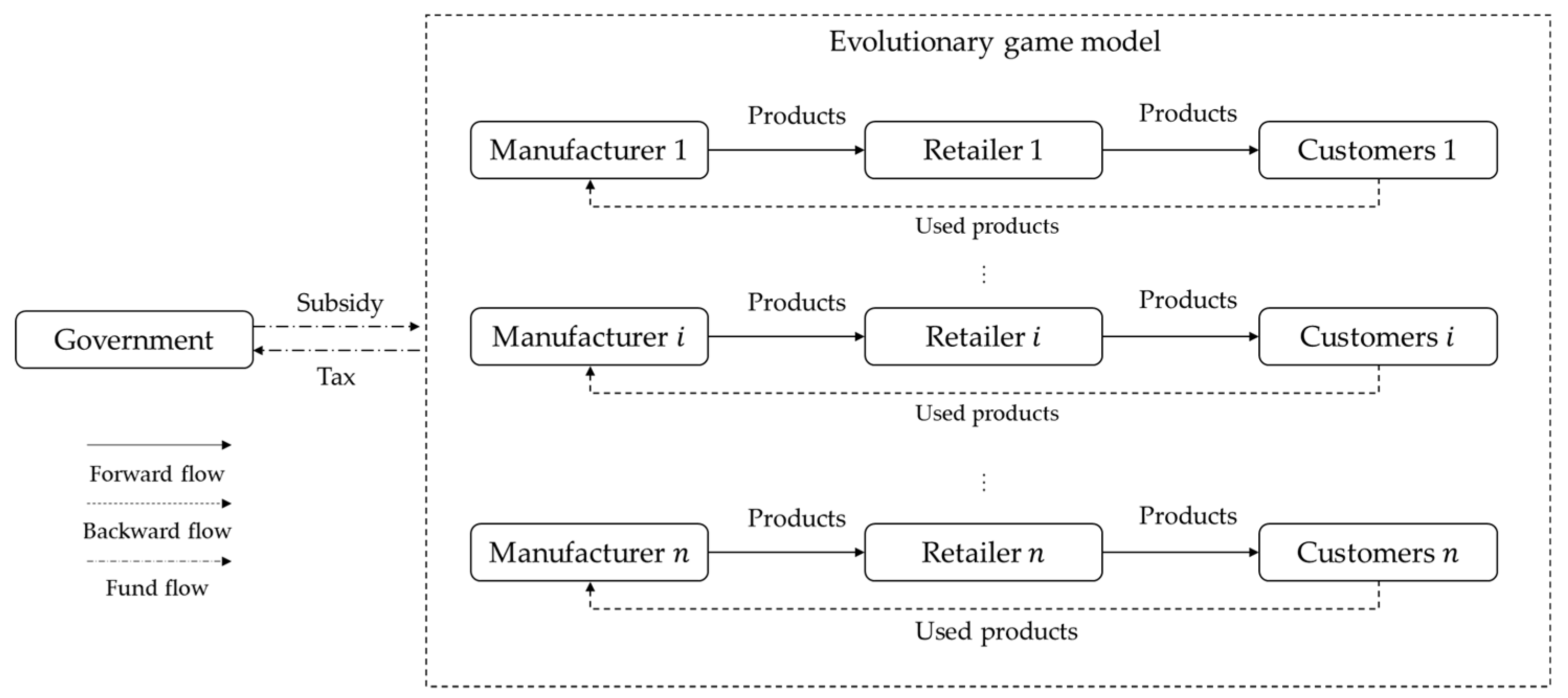
Figure 1 shows an economic system consisting of $n$ supply chains considered in this study. The government can regulate the market at a limited level by taxation and subsidization. Tax and subsidy policies are considered as long-term and one-shot decisions. The policies are decided based on the analysis of the whole market. In this model, a trade-off between economic development and environmental impacts is considered. The government considers both economic development and environmental impacts trying to find the balance between those two. The government collects tax from the manufacturer for all the products and allocates a subsidy for the remanufactured products. Depending on the situation, the government decides the best tax and subsidy policies.

The whole market consisting of a sufficient number of supply chains is considered. Each supply chain consists of one manufacturer, one retailer and many customers. In this paper, $n$ manufacturers and $n$ retailers are considered in the whole market. It is assumed that each supply chain belongs to an independent market that is located in different locations.

Each manufacturer and retailer are randomly matched in a certain local market. This assumption is commonly used in evolutionary game models [31,32,33]. The basic assumption of replicator dynamics is that the probability of a player meeting another player that adopts a certain strategy is equal to the fraction of the population that uses a certain strategy [34]. Therefore, it is usual to assume random pairwise matchings in a large population in evolutionary game theory.

In an evolutionary dynamic process, the frequency distribution of populations that adopt different strategies change over time, in which populations that are associated with better-than-average strategies grow, but those strategies associated with worse-than-average strategies decline [34,35]. At the beginning of the game, the manufacturers and the retailers select strategies based on their preferences. Continually, in each round, they observe the behaviors of other manufacturers and retailers and compare their expected profit with the average profit in the whole market. Through the evolutionary dynamics, strategies that with higher profit will be selected by more and more manufacturers and retailers.

In the local market, the manufacturer produces new products and remanufactures used products. The retailer sells those products to the customers and the customers return a certain number of used products to the retailer or manufacturer. Eventually, the returned products are transferred to the manufacturer for remanufacturing. In each supply chain, the manufacturer announces the wholesale price, and then the retailer decides the retail price. Because we assume that each local market is separate from each other, pricing strategies are independent of the change of population. Therefore, pricing strategy and return policy are considered as one-shot decisions.

Both the manufacturer and the retailer have two strategies; $c$ is to collect the used product, and $n$ is not to collect the used products. The strategies of the manufacturer and the retailer are defined as:

• $M_c$: strategy that the manufacturer collects the used products.
• $M_n$: strategy that the manufacturer does not collect the used products.
• $R_c$: strategy that the retailer collects the used products.
• $R_n$: strategy that the retailer does not collect the used products.

The population of manufacturers that adopt $M_c$ and $M_n$ and retailers that adopt $R_c$ and $R_n$, changes over time.

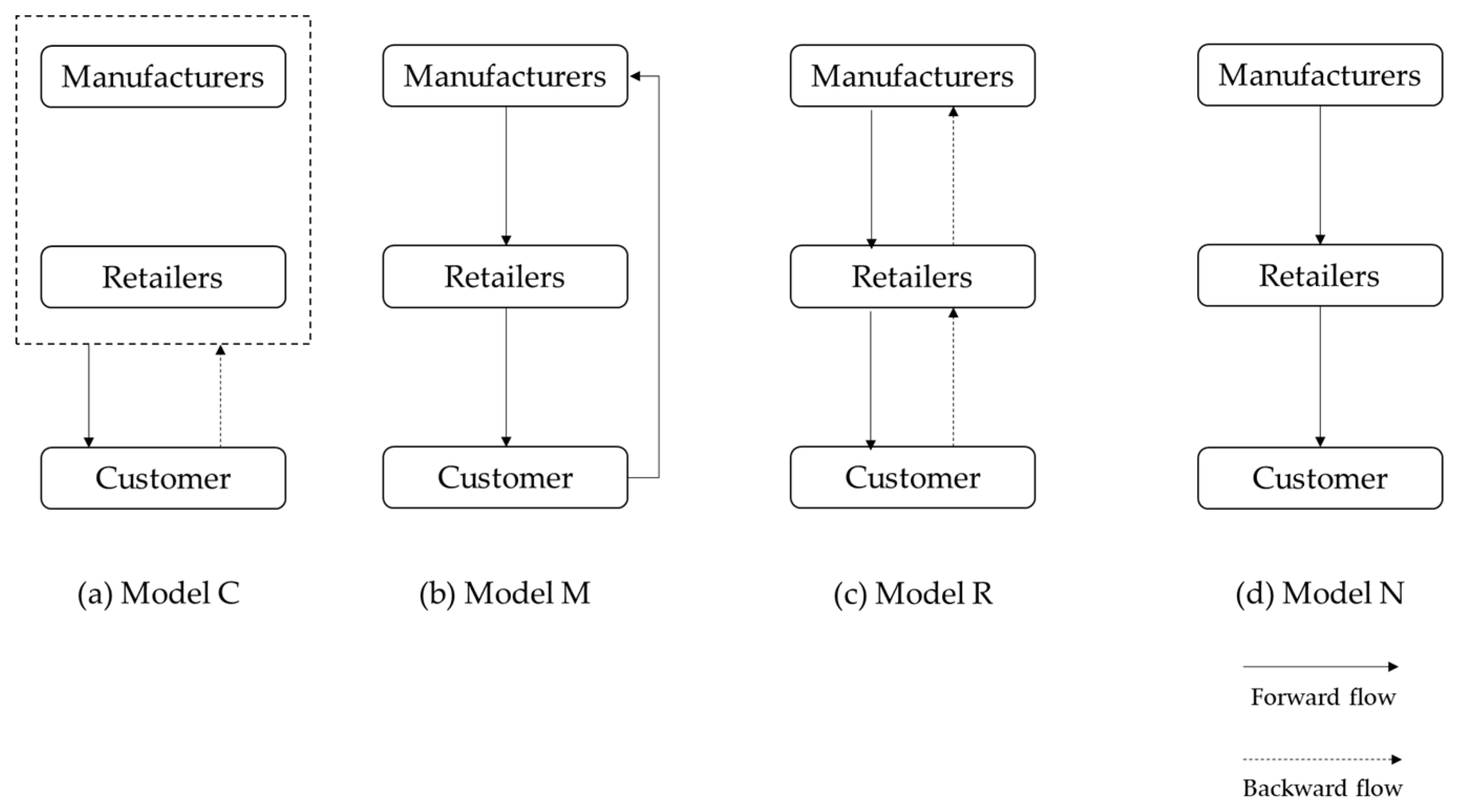
In each closed-loop supply chain, four kinds of channel structures are considered which includes model C, M, R and N as shown in Figure 2. Model C is the centralized supply chain structure, in which the manufacturer and the retailer cooperate with each other to find the optimal pricing and return policies. In model M, the manufacturer directly collects the used products from the customer. In model R, the retailer collects the used products from the customers and recycles those items to the manufacturer. In model N, the recycling and the remanufacturing process are not conducted.

${\mathrm{c}}_{\mathrm{n}}$, ${\mathrm{c}}_{\mathrm{r}}$, $\Delta$, $b$, $\alpha$, $\mathsf{\lambda }$, $e_n$, $e_r$, $N$, $L_j$ are the given parameters. With the returned products, the remanufacturing cost is less than the manufacturing cost ($c_n>c_r>0$). For simplicity, the residual value of a used product is calculated by $\Delta =c_n-c_r$. In model R, the retailer takes charge of collecting used products and transfers those products to the manufacturer. the payment of collection and transportation of the manufacturer is $b$. The manufacturer is profitable when $b\le \Delta$. In model C, one decision-maker optimizes the total profit for both manufacturer and retailer. The profit allocation rate of the manufacturer is $\alpha$. Therefore, the profit of the manufacturer in model C is ${\Pi }_m^C=\alpha {\Pi }^C$, and the profit of the retailer is ${\Pi }_r^C=\left(1-\alpha \right){\Pi }^C$. The manufacturing and remanufacturing processes inevitably have environmental impacts, for example, pollution and raw material consumption. The environmental impacts of the remanufacturing process are equal or less than the manufacturing process ($e_r\le e_n$). $L_j$ is adopted to describe the individual rationality of the manufacturer and the retailer. The players are willing to enter the market only when the average expected profit is larger than their expectations.

Players, models and corresponding decision variables are introduced in

Table 2. Players, models and decision variables.

Players	Models	Decision variables
Government	Optimization (static)	tax and subsidy policies, channel structures
Whole market (multiple manufacturers and retailers)	Evolutionary game model (dynamic)	total quantity of new and remanufactured products, population
Local market (one manufacturer and one retailer)	Stackelberg game model (static)	wholesale and retail price, return policy

.

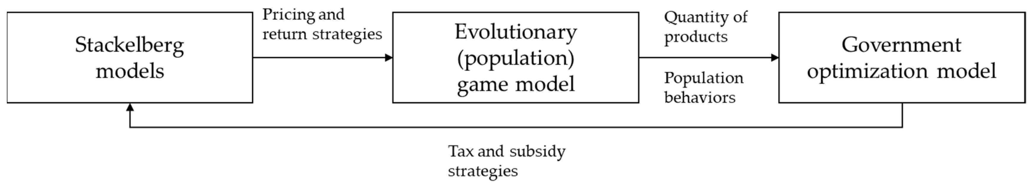
Figure 3 illustrates the relationship between the proposed models. The profit, wholesale price, retail price and return policies of the manufacturer and the retailer in different channel structures are solved by the Stackelberg game model. Based on the profit analysis in the Stackelberg game model, the evolutionary game model is proposed to investigate the total quantity of new and remanufactured products and population behaviors in the whole market. Finally, a government optimization model is proposed to decide the optimal tax and subsidy policies in a closed-loop supply chain.

3.1.3. Assumptions

Assumption 1.

Demand is a linear function of retail price. The demand function is given by:

$$D\left(p\right)=\varnothing -\beta p$$

(1)

where$\varnothing$and$\beta$are positive parameters.$\varnothing$represents the market potential and$\beta$is the consumer’s sensitivity to price.

Assumption 2.

The manufacturer and the retailer can increase the return rate by investing capital in the market, such as advertising. $C_L$ is a parameter that is used to describe how investment affects the return rate. The return rate is given by:

$$\tau =\sqrt{I/C_L}$$

(2)

In practical, firms such as Apple, Hewlett-Packard and Xerox Corporation provide some promotional activities to raise the return rate [36]. Therefore, we assume the return rate depends on the collector’s investment. Similar assumption is wildly used in the study of closed-loop supply chains [7,8,9].

By considering the return rate, the average cost of unit product is given by $c=\left(1-\tau \right)c_n+\tau c_r$, where $\Delta =c_n-c_r$. So, the average cost can be also written as $c=c_n-\tau \Delta$. The demand of new products can then be written as $D_n=\left(1-\tau \right)\left(\varnothing -\beta p\right)$, and demand of remanufactured products can be written as $D_r=\tau \left(\varnothing -\beta p\right)$.

Assumption 3.

In order to make this model more practical, we assume that$C_L$should be large enough so that the optimal return rate is smaller than 1, namely,${\partial \Pi /\partial \tau |}_{\tau =1}<0$. That is, investing loads of money to make the return rate reach 100% is not profitable for the collectors. Similar assumptions can be also found in [7,37,38].

Assumption 4.

In a decentralized closed-loop supply chain model, the manufacturer is the supply chain pricing leader and the retailer is the pricing follower. Commonly, the manufacturer is considered as the supply chain leader and the retailer is the follower, which means that the manufacturer decides the wholesale price first, and then the retailer decides the retail price [7,9,17]. It is also a practical assumption in the real world.

Assumption 5.

We assume perfect substitution between the new and remanufactured products which means that customers cannot tell the difference of quality between those two kinds of products and the new and remanufactured products have the same retail price. This is commonly assumed in the literature related to a closed-loop supply chain [6,7,23,25].

Assumption 6.

The government can influence other decision-maker’s decision at a certain level by financial regulation. We assume that the government can collect tax from new and remanufactured products and allocate subsidy to remanufactured products.

3.2. One-Shot Stackelberg Competition Models in Each Local Market

In a local market, we consider the Stackelberg competition between a manufacturer and a retailer. As shown in Figure 2, Three decentralized closed-loop supply chain structures and one centralized structure (model C) are analyzed. Decentralized structures include manufacturer collection (model M), retailer collection (model R) and non-recycling (model N). Savaskan et al. (2004) [7] proposed the model C, M and R and analyzed the profit functions with one-shot games. In order to compare all the situations, model N is also considered in this paper.

3.2.1. Model C (Centralized)

Model C is a centralized supply chain decision system in which a manufacturer and a retailer cooperate with each other to determine the integrated optimal price policy and return policy together. The decision-maker maximizes the profit for both the manufacturer and retailer. Apart from Savaskan et al.’s (2004) [7] work, government regulation is introduced in our supply chain model. The government collects tax from all the products and allocates subsidy to the remanufactured products. We also assume that the government considers this model as a benchmark model when it makes the tax and subsidy policy. The optimization problem of the decision-maker in the centralized supply chain is expressed as follows:

$${\mathrm{Max}}_{\tau , p} {\Pi }^C=\underset{new products}{\underbrace{\left(1-\tau \right)\left(\varnothing -\beta p\right)\left(p-t-c_n\right)}}+\underset{remanufactured products}{\underbrace{\tau \left(\varnothing -\beta p\right)\left(p-t-c_r+s\right)-C_L{\tau }^2}}$$

(3)

The total profit consists of profit of new products and profit of remanufactured products, where profit of remanufactured products include investment $I=C_L{\tau }^2$ and subsidy. In a centralized supply chain, there is only one decision-maker. Therefore, the wholesale price is not considered in this model.

The profit function can be composed as follows:

$${\mathrm{Max}}_{\tau , p} {\Pi }^C=\left(\varnothing -\beta p\right)\left[p-c_n-t+\tau \left(\Delta +s\right)\right]-C_L{\tau }^2$$

(4)

According to assumption 3, ${\partial {\mathsf{\Pi }}^{\mathrm{C}}/\partial \tau |}_{\tau =1}$ should be smaller than 0. For simplicity, we write this condition as $4C_L>\left(\Delta +s\right)\left[\varnothing -\beta \left(c_n+t\right)\right]+\beta {\left(\Delta +s\right)}^2.$ Because model C is a benchmark in this paper, this condition holds for all the models.

The Hessian matrix of ${\Pi }^C$ is as follows:

$$H_C=\left[\begin{array}{cc}\frac{{\partial }^2{\Pi }^C}{\partial p^2}& \frac{{\partial }^2{\Pi }^C}{\partial p\partial \tau }\\ \frac{{\partial }^2{\Pi }^C}{\partial \tau \partial p}& \frac{{\partial }^2{\Pi }^C}{\partial {\tau }^2}\end{array}\right]=\left[\begin{array}{cc}-2\beta & -\beta \left(\Delta +s\right)\\ -\beta \left(\Delta +s\right)& -2C_L\end{array}\right]$$

(5)

For the concavity of the ${\Pi }^C$, the Hessian matrix should be negative definite. Clearly, $-2\beta <0$ and $-2C_L<0$. Hence, we need $4\beta {\mathrm{C}}_{\mathrm{L}}-{\beta }^2{\left(\Delta +s\right)}^2>0$. According to the assumption above, this last condition is satisfied. Therefore, ${\Pi }^C$ is strictly concave in $\tau$ and $p$.

Calculating the first-order condition, the optimal price and return rate policies are given by:

$${\tau }^{C*}=\frac{\left[\varnothing -\beta (c_n+t\right)]\left(\Delta +s\right)}{4C_L-\beta {\left(\Delta +s\right)}^2}$$

(6)

$$p^{C*}=\frac{2C_L\varnothing +\beta \left(2C_L(c_n+t\right)-\varnothing {\left(\Delta +s\right)}^2)}{\beta \left(4C_L-\beta {\left(\Delta +s\right)}^2\right)}$$

(7)

The optimal profit is as follows:

$${\Pi }^{C*}=\frac{C_L{\left(\varnothing -\beta \left(c_n+t\right)\right)}^2}{\beta \left(4C_L-\beta {\left(\Delta +s\right)}^2\right)}$$

(8)

3.2.2. Model M (Manufacturer Collection)

In the following three decentralized models, we assume that the manufacturer is the supply chain leader and the retailer is the follower. The manufacturer sells the products to the retailer at wholesale price $w$, and the retailer sales the products to the customers at price $p$.

In model M, the manufacturer collects the used products and invests money to promote the return rate. Hence, the manufacturer firstly decides the wholesale price and return rate, and then the retailer decides the sales price to optimize their own profit separately.

The Stackelberg competition problem is given by:

$${\mathrm{Max}}_{w,\tau } {\Pi }_m^M=\underset{new products}{\underbrace{\left(1-\tau \right)\left(\varnothing -\beta p\right)\left(w-t-c_n\right)}}+\underset{remanufactured products}{\underbrace{\tau \left(\varnothing -\beta p\right)\left(w-t-c_r+s\right)-C_L{\tau }^2}}$$

(9)

s.t.

$${\mathrm{Max}}_p {\Pi }_r^M=\underset{new products}{\underbrace{\left(1-\tau \right)\left(\varnothing -\beta p\right)\left(p-w\right)}}+\underset{remanufactured products}{\underbrace{\tau \left(\varnothing -\beta p\right)\left(p-w\right)}}$$

(10)

The Stackelberg competition problem can be composed as follows:

$${\mathrm{Max}}_{w,\tau } {\Pi }_m^M=\left(\varnothing -\beta p\right)\left[w-c_n-t+\tau \left(\Delta +s\right)\right]-C_L{\tau }^2$$

(11)

s.t.

$${\mathrm{Max}}_p {\Pi }_r^M=\left(\varnothing -\beta p\right)\left(p-w\right)$$

(12)

In this model, the manufacturer is the supply chain leader and takes charge of collecting the used products. The investment $C_L{\tau }^2$ is considered in the manufacturer’s problem.

The Stackelberg equilibrium is obtained by the backward reduction. First, by calculating the best response function of the retailer, we obtain:

$$p^{M*}=\frac{\varnothing +\beta w}{2\beta }$$

(13)

Substituting the price policy $p$ in ${\Pi }_m^M$, the wholesale price and return rate is given by:

$$w^{M*}=\frac{-4{\mathrm{C}}_{\mathrm{L}}\varnothing +\beta \varnothing {\left(\Delta +s\right)}^2-4\beta {\mathrm{C}}_{\mathrm{L}}\left(c_n+t\right)}{\beta \left(-8{\mathrm{C}}_{\mathrm{L}}+\beta {\left(\Delta +s\right)}^2\right)}$$

(14)

$${\tau }^{M*}=\frac{\left(\Delta +s\right)\left(-\varnothing +\beta \left(c_n+t\right)\right)}{-8{\mathrm{C}}_{\mathrm{L}}+\beta {\left(\Delta +s\right)}^2}$$

(15)

The Stackelberg equilibrium outcomes for the manufacturer and the retailers are as follows:

$${\Pi }_r^{M*}=\frac{4C_L{}^2{\left(\varnothing -\beta \left(c_n+t\right)\right)}^2}{\beta {\left(8C_L-\beta {\left(\Delta +s\right)}^2\right)}^2}$$

(16)

$${\Pi }_m^{M*}=\frac{C_L{\left(\varnothing -\beta \left(c_n+t\right)\right)}^2}{\beta \left(8C_L-\beta {\left(\Delta +s\right)}^2\right)}$$

(17)

${\Pi }_r^M$ is strictly concave in $p$, because ${\partial }^2{\Pi }_r^M/\partial p^2=-2\beta <0$.

To proof the concavity of ${\Pi }_m^M$, the Hessian matrix is derived:

$$H_M=\left[\begin{array}{cc}\frac{{\partial }^2{\Pi }_m^M}{\partial w^2}& \frac{{\partial }^2{\Pi }_m^M}{\partial w\partial \tau }\\ \frac{{\partial }^2{\Pi }_m^M}{\partial \tau \partial w}& \frac{{\partial }^2{\Pi }_m^M}{\partial {\tau }^2}\end{array}\right]=\left[\begin{array}{cc}-\beta & -\frac{1}{2}\beta \left(\Delta +s\right)\\ -\frac{1}{2}\beta \left(\Delta +s\right)& -2C_L\end{array}\right]$$

(18)

$H_M$ is negative definite and hence ${\Pi }_m^M$ is strictly concave in $\tau$ and $w$, because $-\beta <0$, $-2C_L<0$ and $2C_L\beta -{\beta }^2{\left(\Delta +s\right)}^2/4>0$. The third inequality is satisfied by the assumption of $C_L$.

3.2.3. Model R (Retailer Collection)

In this model, the retailer collects the used products and sales of those items to the manufacturer at price $b$. Similar to the previous model, the manufacturer firstly decides the wholesale price $w$, then the retailer decides the retail price and investment, since the retailer is in charge of the collection.

The optimization problems are formulated as follows:

$${\mathrm{Max}}_w {\Pi }_m^R=\underset{new products}{\underbrace{\left(1-\tau \right)\left(\varnothing -\beta p\right)\left(w-t-c_n\right)}}+\underset{remanufactured products}{\underbrace{\tau \left(\varnothing -\beta p\right)\left(w-t-c_r+s-b\right)}}$$

(19)

s.t.

$${\mathrm{Max}}_{p, \tau } {\Pi }_r^R=\underset{new products}{\underbrace{\left(1-\tau \right)\left(\varnothing -\beta p\right)\left(p-w\right)}}+\underset{remanufactured products}{\underbrace{\tau \left(\varnothing -\beta p\right)\left(p-w+b\right)-C_L{\tau }^2}}$$

(20)

The Stackelberg competition problem can be written as follows:

$${\mathrm{Max}}_w {\Pi }_m^R=\left(\varnothing -\beta p\right)\left[w-c_n-t+\tau \left(\Delta +s-b\right)\right]$$

(21)

s.t.

$${\mathrm{Max}}_{p, \tau } {\Pi }_r^R=\left(\varnothing -\beta p\right)\left(p-w+b\tau \right)-C_L{\tau }^2$$

(22)

By the idea of backward reduction, we derive the sale price and return rate from the retailer’s best-response function firstly as follows:

$$p^{R*}=\frac{b^2\beta \varnothing -2{\mathrm{C}}_{\mathrm{L}}\varnothing -2{\mathrm{C}}_{\mathrm{L}}\beta w}{\beta \left(b^2\beta -4{\mathrm{C}}_{\mathrm{L}}\right)}$$

(23)

$${\tau }^{R*}=\frac{-b\varnothing +b\beta w}{b^2\beta -4{\mathrm{C}}_{\mathrm{L}}}$$

(24)

Substituting $p^{R*}$ and ${\tau }^{R*}$ in ${\Pi }_m^R$, the optimal wholesale price of the manufacturer is given by:

$$w^{R*}=\frac{2b\beta \varnothing \left(\Delta +s\right)+b^2\beta \left(-\varnothing +\beta \left(c_n+t\right)\right)-4{\mathrm{C}}_{\mathrm{L}}\left(\varnothing +\beta \left(c_n+t\right)\right)}{2\beta \left(-4{\mathrm{C}}_{\mathrm{L}}+b\beta \left(\Delta +s\right)\right)}$$

(25)

The Stackelberg equilibrium for the manufacturer and the retailers are as follows:

$${\Pi }_r^{R*}=\frac{\left(4C_L-b^2\beta \right)C_L{\left(\varnothing -\beta \left(c_n+t\right)\right)}^2}{4\beta {\left(4C_L-b\beta \left(\Delta +s\right)\right)}^2}$$

(26)

$${\Pi }_m^{R*}=\frac{C_L{\left(\varnothing -\beta \left(c_n+t\right)\right)}^2}{2\beta \left(4C_L-b\beta \left(\Delta +s\right)\right)}$$

(27)

To proof the concavity of ${\Pi }_r^R$, the Hessian matrix is derived:

$$H_R=\left[\begin{array}{cc}\frac{{\partial }^2{\Pi }_r^R}{\partial p^2}& \frac{{\partial }^2{\Pi }_r^R}{\partial p\partial \tau }\\ \frac{{\partial }^2{\Pi }_r^R}{\partial \tau \partial p}& \frac{{\partial }^2{\Pi }_r^R}{\partial {\tau }^2}\end{array}\right]=\left[\begin{array}{cc}-2\beta & -b\beta \\ -b\beta & -2C_L\end{array}\right]$$

(28)

$H_R$ is negative definite and hence ${\Pi }_r^R$ is strictly concave in $\tau$ and $p$, because $-2\beta <0$, $-2C_L<0$ and $4{\mathrm{C}}_{\mathrm{L}}\beta -b^2{\beta }^2>0$. The third inequality is satisfied by the assumption of $C_L$.

${\Pi }_m^R$ is also concave since ${\partial }^2{\mathsf{\Pi }}_m^{\mathrm{R}}/\partial w^2=4\beta {\mathrm{C}}_{\mathrm{L}}\left(b\beta \left(\Delta +s\right)-4{\mathrm{C}}_{\mathrm{L}}\right)/{\left(b^2\beta -4{\mathrm{C}}_{\mathrm{L}}\right)}^2<0$.

3.2.4. Model N (Non-Recycling)

In order to conduct a comparative study on the closed-loop supply chain, in model N, we consider a special case neither the manufacturer nor the retailer collects the used products. So, return rate $\tau$ is irrelevant. Still, the manufacturer is the supply chain leader and firstly announces the wholesale price, then the retailer decides the sale price.

The Stackelberg competition problem is given by:

$${\mathrm{Max}}_w {\Pi }_m^N=\left(w-c_n-t\right)\left(\varnothing -\beta p\right)$$

(29)

s.t.

$${\mathrm{Max}}_p {\Pi }_r^N=\left(p-w\right)\left(\varnothing -\beta p\right)$$

(30)

Calculating the first-order condition, the best-response of the retailer is as follows:

$$p^{N*}=\frac{\varnothing +\beta w}{2\beta }$$

(31)

Substituting $p^{N*}$ in ${\Pi }_m^N$, and the optimal wholesale price of the manufacturer is derived by

$$w^{N*}=\frac{\beta c_n+\varnothing +\beta t}{2\beta }$$

(32)

The Stackelberg equilibrium outcomes for the manufacturer and the retailers are as follows:

$${\Pi }_r^{N*}=\frac{{\left(\varnothing -\beta \left(c_n+t\right)\right)}^2}{16\beta }$$

(33)

$${\Pi }_m^{N*}=\frac{{\left(\varnothing -\beta \left(c_n+t\right)\right)}^2}{8\beta }$$

(34)

${\Pi }_r^N$ is concave in $p$, because ${\partial }^2{\mathsf{\Pi }}_r^{\mathrm{N}}/\partial p^2=-2\beta <0$. ${\Pi }_m^{N*}$ is concave in $w$, because ${\partial }^2{\mathsf{\Pi }}_m^{\mathrm{N}}/\partial w^2=-\beta <0$.

3.3. Evolutionary Game Model

3.3.1. Model Description

In this section, the dynamic population game is used to describe the whole market and how it changes over time and is developed by adopting an evolutionary game theory. A big market that consists of many local markets is considered and in each local market, the manufacturer and the retailer play the one-shot Stackelberg models.

In this game, each manufacturer and retailer can choose to collect the used products or not collect the used products. $M_c$ and $M_n$ are respectively used to describe those two strategies of each manufacturer, and $R_c$, $R_n$ for retailers. Then, four strategy combinations are obtained, which correspond to the results of Stackelberg competition between one manufacturer and one retailer in the previous section. The payoff matrix of the evolutionary game is shown in

Table 3. Payoff matrix.

Manufacturer	Retailer
	${\mathit{R}}_{\mathit{c}}$	${\mathit{R}}_{\mathit{n}}$
$M_c$	${\Pi }_m^{C*}$,${\Pi }_r^{C*}$	${\Pi }_m^{M*}$,${\Pi }_r^{M*}$
$M_n$	${\Pi }_m^{R*}$,${\Pi }_r^{R*}$	${\Pi }_m^{N*}$,${\Pi }_r^{N*}$

* indicates the optimal solution (Stackelberg equilibrium).

. The expression of each payoff can be found in Section 3.2.

To describe the change of population over time, $x$ and $y$ are adopted. Let x represent the proportion of manufacturers who select strategy $M_c$. Then, $\left(1-x\right)$ is the fraction of the manufacturers who choose strategy $M_n$. Similarly, we use $y$ to represent the proportion of the retailers who select strategy $R_c$, and use $\left(1-y\right)$ to represent who choose $R_n$. Accordingly, $\left(x, y\right)\in \left[0,1]\times [0,1\right]$. During the evolutionary game process, manufacturers and retailers adjust their strategies, $x$ and $y$ will change over time until the system achieves a steady state.

The expected profit of manufacturers that choose $M_c$ and $M_n$ are set as $E_c^m$ and $E_n^m$, and it can be expressed as

$$E_c^m=y{\Pi }_m^{C*}+\left(1-y\right){\Pi }_m^{M*}$$

(35)

$$E_n^m=y{\Pi }_m^{R*}+\left(1-y\right){\Pi }_m^{N*}$$

(36)

The average expected payoff of manufacturer is:

$$\overline{EM}=x{E}_c^m+\left(1-x\right)E_n^r$$

(37)

The expected profit of retailers that choose $R_c$ and $R_n$ are set as $E_c^r$ and $E_n^r$, and it can be expressed as:

$$E_c^r=x{\Pi }_r^{C*}+\left(1-x\right){\Pi }_r^{R*}$$

(38)

$$E_n^r=x{\Pi }_r^{M*}+\left(1-x\right){\Pi }_r^{N*}$$

(39)

Then, the average expected payoff of retailer is:

$$\overline{ER}=y{E}_c^r+\left(1-y\right)E_n^r$$

(40)

The demand matrix of new products and remanufactured products in each closed-loop supply chain model is shown in

Table 4. Demand matrix.

Manufacturer	Retailer
	${\mathit{R}}_{\mathit{c}}$	${\mathit{R}}_{\mathit{n}}$
$M_c$	$D_n^{C*}, D_r^{C*}$	$D_n^{M*}, D_r^{M*}$
$M_n$	$D_n^{R*}, D_r^{R*}$	$D_n^{N*}, D_r^{N*}$

. Note that the demand of remanufactured products in model N equals 0.

$ED{N}_c$ and $ED{N}_n$ are the expected demand of new products when the manufacturer selects $M_c$ and $M_n$ strategies, respectively. The expressions of $ED{N}_c$ and $ED{N}_n$ are shown as follows:

$$ED{N}_c=y{D}_n^{C*}+\left(1-y\right)D_n^{M*}$$

(41)

$$ED{N}_n=y{D}_n^{R*}+\left(1-y\right)D^{N*}$$

(42)

Therefore, the average demand of new products of manufacturers $\overline{ADN}$ can be calculated by:

$$\overline{ADN}=xED{N}_C+\left(1-x\right)ED{N}_n$$

(43)

$ED{R}_c$ and $ED{R}_n$ are the expected demand of the remanufactured products when the manufacturer selects $M_c$ and $M_n$ strategies, respectively. The expressions of $ED{R}_c$ and $ED{R}_n$ are shown as follows.

$$ED{R}_c=y{D}_r^{C*}+\left(1-y\right)D_r^{M*}$$

(44)

$$ED{R}_n=y{D}_r^{R*}$$

(45)

Therefore, the average demand for remanufactured products of manufacturers $\overline{ADR}$ is shown as follows.

$$\overline{ADR}=xED{R}_c+\left(1-x\right)ED{R}_n$$

(46)

We consider that there are $N$ manufacturers in the whole market. $Q_n$ is the total quantity of new products and $Q_r$ is the total quantity of remanufactured products. $Q_n$ and $Q_r$ can be expressed as:

$$Q_n=N\times \overline{ADN}$$

(47)

$$Q_r=N\times \overline{ADR}$$

(48)

According to the analysis above, the replicator dynamic equations of the closed-loop supply chain model are as follows:

$$\dot{x}=\frac{dx}{dt}=x\left(E_c^m-\overline{EM}\right)=x\left(1-x\right)\left(E_c^m-E_r^m\right)$$

(49)

$$\dot{y}=\frac{dy}{dt}=y\left(E_c^r-\overline{ER}\right)=y\left(1-y\right)\left(E_c^r-E_n^r\right)$$

(50)

Equations in (49) and (50), respectively illustrate the rate of proportion change over time between manufacturers and retailers.

3.3.2. Stability Analysis

In this section, the steady-states and the stability of strategies are analyzed. In an evolutionary game model, a steady-state does not change in time, and the stability means that if a solution starts from near the stationary solution, then it will stay near the solution as time progresses. Moreover, an asymptotic stability means that if a solution starts from a near enough to the stationary solution, then it will eventually converge to the solution [39]. A strategy is an evolutionarily stable strategy (ESS), if and only if the strategy is an asymptotically stable stationary solution [39]. Therefore, the asymptotic stability is analyzed in this paper.

Proposition 1.

(1, 1), (1, 0), (0, 1) and (0, 0) are steady-states.

Proof of Proposition 1.

The dynamic system is stable when the differential equations satisfy:

$$\{\begin{array}{c}\dot{x}=0\\ \dot{y}=0\end{array}$$

(51)

Obviously, (1, 1), (1, 0), (0, 1) and (0, 0) are steady-states. □

Proposition 2.

The steady-state (1, 1) is asymptotic stable.

Proof of Proposition 2.

The Jacobian matrix is adopted to analyze the asymptotic stability of those steady-states. Based on the replicator dynamic equations, the Jacobian matrix of this closed-loop supply chain model is obtained as follows:

$$J=\left[\begin{array}{c}\frac{\partial \dot{x}}{\partial x}\\ \frac{\partial \dot{y}}{\partial x}\end{array} \begin{array}{c}\frac{\partial \dot{x}}{\partial y}\\ \frac{\partial \dot{y}}{\partial x}\end{array}\right]$$

(52)

A steady-state is asymptotic stable if the trace of the Jacobian matrix is less than 0 ($\mathrm{tr}\left(J\right)<0$) and the determinant of the Jacobian matrix is larger than 0 ($\det \left(J\right)>0$), where

$$\mathrm{tr}\left(J\right)=\frac{\partial \dot{x}}{\partial x}+\frac{\partial \dot{y}}{\partial x}$$

(53)

$$\det \left(J\right)=\frac{\partial \dot{x}}{\partial x}\frac{\partial \dot{y}}{\partial x}-\frac{\partial \dot{x}}{\partial y}\frac{\partial \dot{y}}{\partial x}$$

(54)

According to the model description, $\mathrm{b}\le \Delta$ and $\mathrm{s}>0$, then we can get $b<\Delta +s$.

Hence,

$${\Pi }_m^{R*}=\frac{{\left(\varnothing -\beta \left(c_n+t\right)\right)}^2/8\beta }{1-b\beta \left(\Delta +s\right)/4C_L}<\frac{{\left(\varnothing -\beta \left(c_n+t\right)\right)}^2/8\beta }{1-\beta {\left(\Delta +s\right)}^2/4C_L}$$

Then

$${\Pi }^{C*}-{\Pi }_r^{M*}-{\Pi }_m^{R*}$$

$$>{\Pi }^{C*}-{\Pi }_r^{M*}-\frac{{\left(\varnothing -\beta \left(c_n+t\right)\right)}^2/8\beta }{1-\beta {\left(\Delta +s\right)}^2/4C_L}$$

$$=\frac{C_L\left(\frac{C_L\left(32C_L-8\beta {\left(\Delta +s\right)}^2\right)+{\beta }^2{\left(\Delta +s\right)}^4}{\left(4C_L-\beta {\left(\Delta +s\right)}^2\right){\left(-8C_L+\beta {\left(\Delta +s\right)}^2\right)}^2}\right){\left(\varnothing -\beta \left(c_n+t\right)\right)}^2}{2\beta }$$

According to the assumption, $4{\mathrm{C}}_{\mathrm{L}}>\left(\Delta +\mathrm{s}\right)\left[\varnothing -\mathsf{\beta }\left({\mathrm{c}}_{\mathrm{n}}+\mathrm{t}\right)\right]+\mathsf{\beta }{\left(\Delta +\mathrm{s}\right)}^2$, we obtain,

$$32C_L-8\beta {\left(\Delta +s\right)}^2$$

$$>8\left(\Delta +s\right)\left[\varnothing -\beta \left(c_n+t\right)\right]+8\beta {\left(\Delta +s\right)}^2-8\beta {\left(\Delta +s\right)}^2>0$$

Therefore,

$${\Pi }^{C*}-{\Pi }_r^{M*}-{\Pi }_m^{R*}>0$$

Exist $0<\alpha <1$ that makes ${\Pi }_m^{C*}$, ${\Pi }_r^{C*}$ satisfy

$$\alpha {\Pi }^{C*}+\left(1-\alpha \right){\Pi }^{C*}>{\Pi }_r^{M*}+{\Pi }_m^{R*}$$

$${\Pi }_m^{C*}=\alpha {\Pi }^{C*}>{\Pi }_m^{R*}$$

$${\Pi }_r^{C*}=\left(1-\alpha \right){\Pi }^{C*}>{\Pi }_r^{M*}$$

Finally,

$$\mathrm{tr}\left(\mathrm{J}\right)=\left({\Pi }_m^{R*}-{\Pi }_m^{C*}\right)+\left({\Pi }_r^{M*}-{\Pi }_r^{C*}\right)<0$$

$$\det \left(\mathrm{J}\right)=\left({\Pi }_m^{R*}-{\Pi }_m^{C*}\right)\left({\Pi }_r^{M*}-{\Pi }_r^{C*}\right)>0$$

Therefore, (1, 1) is an ESS. □

Proposition 3.

The steady-state (0, 0) is unstable.

Proof of Proposition 3.

Firstly, we calculate:

$${\Pi }_m^{M*}-{\Pi }_m^{N*}=\frac{{\left(\varnothing -\beta \left(c_n+t\right)\right)}^2}{\beta \left(8-\beta {\left(\Delta +s\right)}^2/C_L\right)}-\frac{{\left(\varnothing -\beta \left(c_n+t\right)\right)}^2}{8\beta }$$

We have $\beta {\left(\Delta +s\right)}^2/C_L>0$, hence, ${\Pi }_m^{M*}-{\Pi }_m^{N*}>0$.

Secondly,

$${\Pi }_r^{R*}=\frac{\left(4C_L-b^2\beta \right)C_L{\left(\varnothing -\beta \left(c_n+t\right)\right)}^2}{4\beta {\left(4C_L-b\beta \left(\Delta +s\right)\right)}^2}$$

$$>\frac{\left(4C_L-b^2\beta \right)C_L{\left(\varnothing -\beta \left(c_n+t\right)\right)}^2}{4\beta {\left(4C_L-b^2\beta \right)}^2}$$

$$=\frac{{\left(\varnothing -\beta \left(c_n+t\right)\right)}^2}{16\beta -4b^2{\beta }^2/C_L}$$

we can obtain:

$${\Pi }_r^{R*}-{\Pi }_r^{N*}$$

$${\Pi }_r^{R*}-{\Pi }_r^{N*}>\frac{{\left(\varnothing -\beta \left(c_n+t\right)\right)}^2}{16\beta -4b^2{\beta }^2/C_L}-\frac{{\left(\varnothing -\beta \left(c_n+t\right)\right)}^2}{16\beta }$$

We have $4b^2{\beta }^2/C_L>0$, hence, ${\Pi }_r^{R*}-{\Pi }_r^{N*}>0$.

Finally,

$$\mathrm{trJ}={\Pi }_m^{M*}-{\Pi }_m^{N*}+{\Pi }_r^{R*}-{\Pi }_r^{N*}>0$$

$$\mathrm{detJ}=\left[{\Pi }_m^{M*}-{\Pi }_m^{N*}\right]\left[{\Pi }_r^{R*}-{\Pi }_r^{N*}\right]>0$$

Therefore, (0, 0) is unstable point. □

Proposition 4.

The steady-state (1, 0) is unstable.

Proof of Proposition 4.

Because ${\Pi }_r^{C*}>{\Pi }_r^{M*}$ and ${\Pi }_m^{M*}>{\Pi }_m^{N*}$, clearly, $\mathrm{detJ}=\left[{\Pi }_m^{N*}-{\Pi }_m^{M*}\right]\left[{\Pi }_r^{C*}-{\Pi }_r^{M*}\right]<0$.

Therefore, (1, 0) is unstable. □

Proposition 5.

The steady-state (0, 1) is unstable.

Proof of Proposition 5.

Because ${\Pi }_m^{C*}>{\Pi }_m^{R*}$ and ${\Pi }_r^{R*}>{\Pi }_r^{N*}$, clearly, $\mathrm{detJ}=\left[{\Pi }_m^{R*}-{\Pi }_m^{C*}\right]\left[{\Pi }_r^{R*}-{\Pi }_r^{N*}\right]<0$.

Therefore, (0, 1) is unstable. □

According to the propositions, the results are summarized in

Table 5. Stability of equilibrium points.

Equilibrium Point	$\mathbf{det}\left(\mathbf{J}\right)$	$\mathbf{tr}\left(\mathbf{J}\right)$	Local Stability
(0, 0)	+	+	Unstable
(0, 1)	−		Unstable
(1, 0)	−		Unstable
(1, 1)	+	-	ESS

. (1, 1) is the evolutionarily stable strategy (ESS).

3.4. Government Model

A government model based on the results of the Stackelberg competition model in the local market and the evolutionary analysis in the whole market is developed. By collecting taxes from all products and allocating subsidies to remanufacturing products, the government can regulate the market to a certain level. To obtain the optimal policies, the trade-off between public revenue and environment impacts is analyzed in the optimization model.

The total public revenue $PR$ is calculated by tax and subsidies:

$$PR=t\left(Q_n+Q_r\right)-s{Q}_r$$

(55)

The environmental impact $EI$ is calculated as:

$$EI=e_n{Q}_n+e_r{Q}_r$$

(56)

The government’s revenue consists of public revenue and environmental impact. $\mathsf{\lambda }$ represents how much the government cares about the environment. The government’s optimization problem is formulated as follows:

$${\mathrm{Max}}_{x, y,t,s} \left(1-\lambda \right)PR-\lambda EI$$

(57)

Subject to:

$$p^{i*}>C_n, \forall i$$

(58)

$$0\le {\tau }^{i*}\le 1, \forall i$$

(59)

$$0\le t\le 0.2p^{C*}$$

(60)

$$0\le s\le 0.1p^{C*}$$

(61)

$$\overline{EM}\ge L_m$$

(62)

$$\overline{ER}\ge L_r$$

(63)

$$0\le x, y\le 1$$

(64)

The objective function (57) consists of the weighted profit of the total public revenue and the reduction of the environmental impact. Constraints (58) represent the fact that the sale price should be larger than the cost of producing a new product. In Section 3.2, the pricing strategies in four models have been derived and these strategies depend on the government tax and subsidy policies. These constraints prevent the situation of the sale price being larger than the cost under government regulations. Constraints (59) represent the recycle rate should between 0 and 1. These constraints ensure that the quantity of returned products is smaller than the quantity of new products and the return rate should be positive. 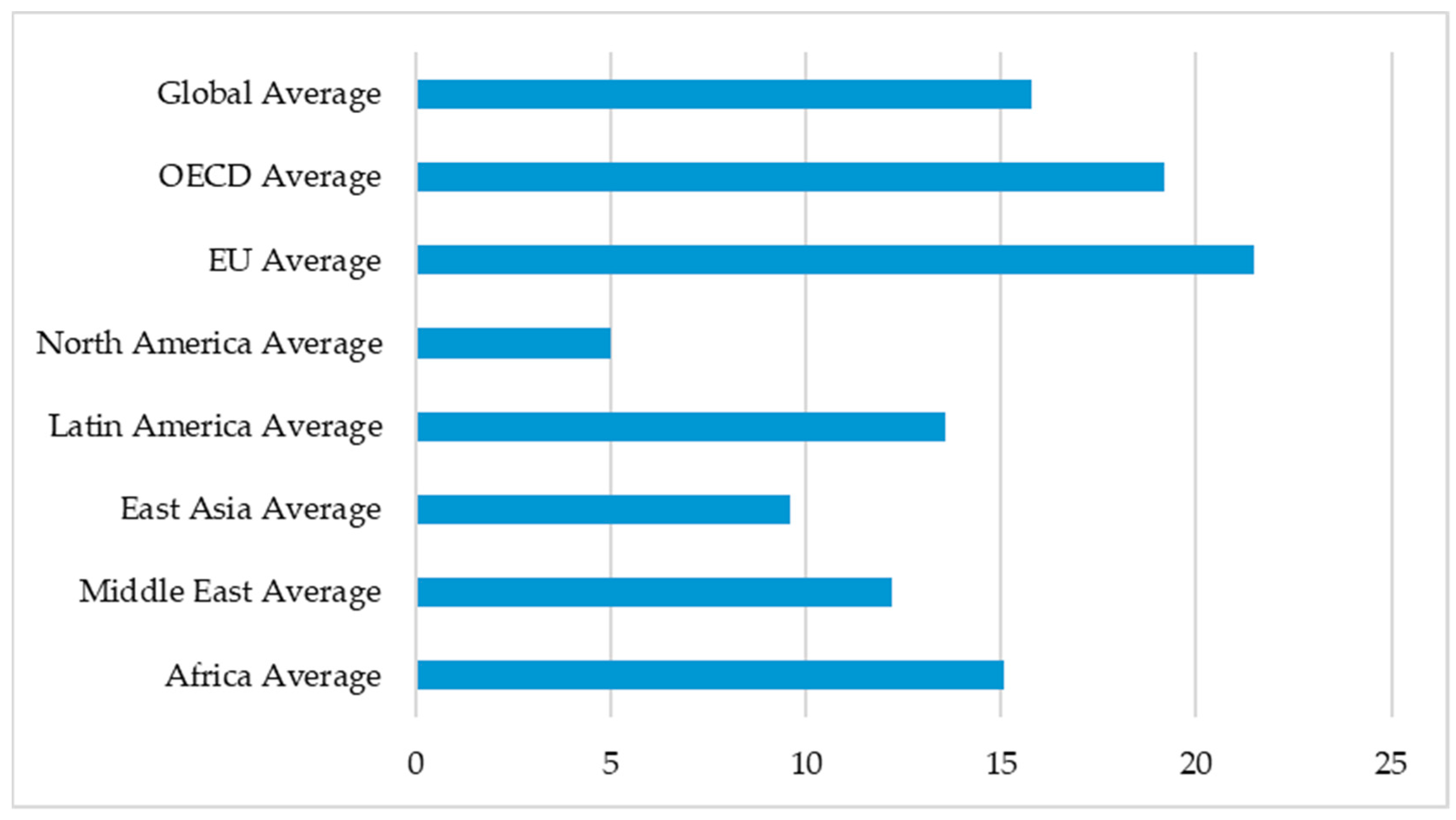Figure 4 shows the standard value-added tax (VAT)/sales tax rates around the world in 2014. In most areas of the world, the standard tax rates are lower than 20%, and the global average rate is 15.8%. Hence, in constraints (60), the tax of unit product is limited to 20% of the basic sale price. In 2009, China’s subsidy for home appliance replacements is 10% of the price. So, in constraints (61), subsidy of unit remanufactured product is limited to 10% of the sale price. Constraints (60) and (61) ensure that the government can regulate the market at a reasonable level. Constraints (62) and (63) represent the fact that the expected profits of the manufacturers and the retailers should be larger than the lower bounds of profit under government regulation. These constraints indicate that when the government makes decisions, it should consider the expected profit of the manufacturers and the retailers. Constraints (64) are the variable boundary conditions which indicate that the fraction of the manufacturer population and the retailer population should be larger than 0 and smaller than 1. These constraints are derived from the evolutionary game model.

4. Numerical Experiments

To illustrate the proposed model, numerical experiments are conducted in this section. Based on data from the literature related to closed-loop supply chain [8] and practical assumptions. The assumed values of the baseline parameter are shown in

Table 6. Baseline parameter values.

Market size	$\varnothing$	100
Price sensitivity	$\beta$	0.3
Scale parameter	$C_L$	1000
Production cost	$c_n$	20
Number of manufacturers	$N$	100
Allocation rate	$\alpha$	0.6671
Environmental impact (new)	$e_n$	15
Environmental impact (used)	$e_r$	2
Residual value	$\Delta$	15
Collection cost	$b$	15
Environmental attention	$\lambda$	0.7
Expected profit of manufacturer	$L_m$	0
Expected profit of retailer	$L_r$	0

. The values of $\varnothing$, $\beta$, $c_n$, $\Delta$ are gathered from [8]. The reason that we assume $C_L=1000$ is according to assumption 3, the scale parameter $C_L$ should be large enough so that the optimal return rate is lower than 1. Also, to have enough of a population in the evolutionary process, 100 manufacturers and retailers are assumed. According to the proof in stability analysis, there exist $\alpha$ that makes the centralized supply chain structurer stable. Based on the preliminary experiments, we assume $\alpha =0.6671$. The values for $e_n$ and $e_r$ are based on [26]. In their paper, the environmental impact of remanufactured products $e_r$ is calculated by $\rho e_n$, where $\rho$ is a parameter that is larger than 0 and equal or less than 1. Hence, in our paper, the environmental impact of remanufacturing unit used product should be smaller or equal to the environmental impact of producing a new product. Therefore, we assume that $e_n=15$ and $e_r=2$. $b$ is the price that the manufacturer pays to the retailers for collecting used products and we assume $b\le \Delta$. The profit of the manufacturer in model R is increased with respect to $b$. To maximize their profit, in the following examples, we assume that $b=\Delta$. $L_m$ and $L_r$ are the lower bound of the expected profits. We assume that $L_m=0$ and $L_r=0$, indicating that the manufacturers and retailers are willing to enter the market as long as they do not lose money in the market. We assume $\lambda =0.7$, which means that the government cares more about environmental issues than public revenue. In order to examine the effects of the main parameters, the different values for $\Delta$, $b$, $\lambda$, $e_r$ and $\left(L_m, L_r\right)$ will be taken in the numerical experiments.

4.1. Analysis of Tax and Subsidy

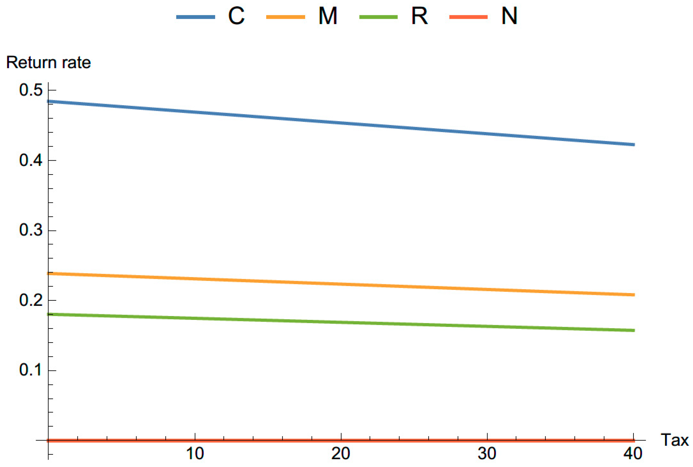
To examine how tax influences the return rates and demand for new products in different models, we set $s=5$ in Figure 5 and Figure 6.

Figure 5 demonstrates that the return rates decrease in model C, M and R with the tax, while the return rate in model N keeps at 0. Although taxes are collected from all products, it has impacts on return rates in some models. In assumption 2 and assumption 3, we assume that the investment to return rate is $I=C_L{\tau }^2$ and $C_L$ is sufficiently large so that the optimal return rate is smaller than 1. Therefore, collectors should invest relatively higher investment to increase the return rate. In this example, the higher tax leads to higher retail price and lower profits. With lower profit, the firm will decrease the investment to return rate. As a result, when governments increase the tax, the collectors choose to decrease the investment and the return rates also decrease.

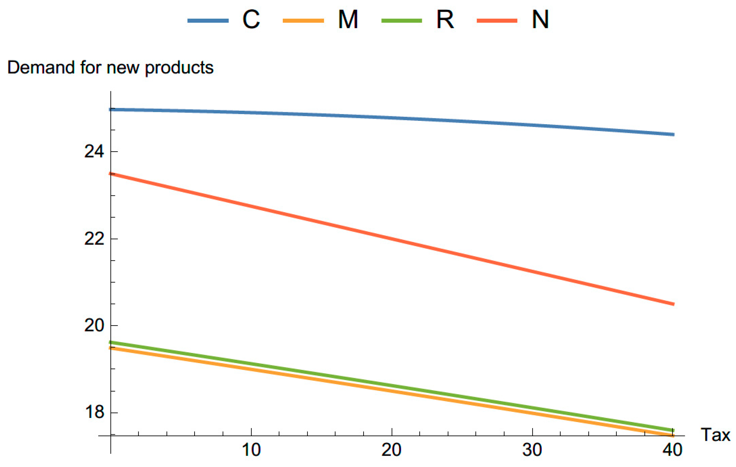
Figure 6 shows that the demand for new products decreases with the increase of tax in all channel structures. The reason is that high tax leads to high retail price and low demand. Therefore, by increasing tax, the demand of new products is decreased and the environmental impact of production is also decreased. Also, as shown in Figure 6, the demand of new products in model C is less sensitive to the change of tax compared with other models M, R and N.

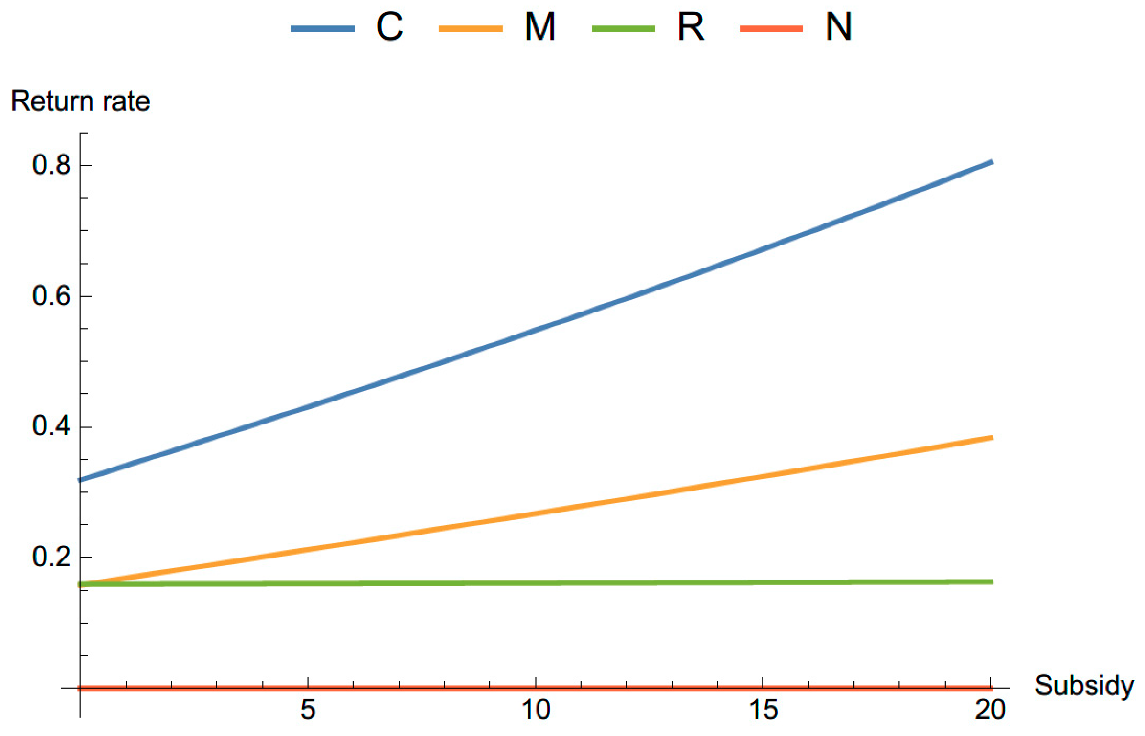
Figure 7 and Figure 8 show, how subsidy influences the return rates and demand for remanufactured products when we set $t=35$.

In Figure 7, as the subsidy increases, the return rates in model C and M increase. However, the return rate in model R is not sensitive to the change of subsidy. The subsidy is allocated to the manufacturer to improve the remanufacturing process. However, in model R, the retailers take charge of investment and collecting the used products. To maximize their profit, the manufacturers choose to keep the subsidy instead of reallocating the subsidy to the retailers. As a result, the subsidy cannot effectively enhance the return rate in model R.

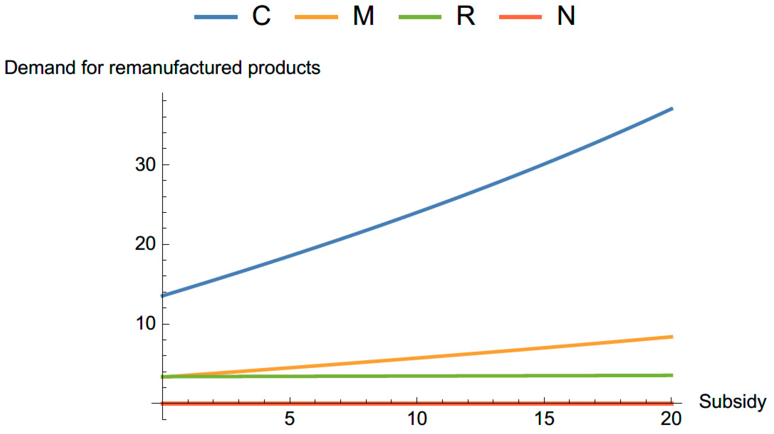
In Figure 8, the demand for remanufactured products increases with the increase of subsidy in model C and R. The demand of used products in model C is more sensitive to the change of subsidy comparing with other models. In this paper, we assume that the environmental impacts of the remanufacturing process are less than the manufacturing process $\left({\mathrm{e}}_{\mathrm{r}}\le {\mathrm{e}}_{\mathrm{n}}\right)$. Therefore, by increasing subsidy, the government can collect more tax to reduce the environmental impacts of production.

4.2. Analysis of Evolutionary Dynamics

In Section 3.3.2, we have proved that only the centralized supply chain is a stable strategy in this model. Here, we use an example to illustrate the evolutionary dynamics of the manufacturers and retailers with four different channel structures. This example also provides a benchmark case to study the effects of the main parameters of our model. In Section 4.3, the results derived from this example will be compared with other scenarios, in which the main parameters take different values. The values of parameters in this example are listed in Table 6.

To analyze the evolutionary process, we solve the government optimization model to derive the optimal tax and subsidy policies. Then, the results of the government model are substituted into the Stackelberg competition models to obtain the price and return rate policies of the manufacturers and retailers in different channel structures. The results of the government model and Stackelberg competition model are listed in

Table 7. Government tax and subsidy policies.

$t$	37.3194	$EI$	38922.3878
$s$	13.1639	$PR$	128360.9928
$\overline{EM}$	4052.7609	$x$	1
$\overline{ER}$	2022.4316	$y$	1

and

Table 8. Pricing, return policies and profits of manufacturers and retailers.

	Model C	Model M	Model R	Model N
${\Pi }_m^{*}$	4052.7609	2944.4723	2950.3691	2856.8884
${\Pi }_r^{*}$	2022.4316	1517.3707	1497.746	1428.4442
$p^{*}$	186.597	262.2144	262.072	264.3299
$D^{*}$	44.0209	21.3357	21.3784	20.701
${\tau }^{*}$	0.6199	0.30045	0.16034	0

.

Under these parameters, the Hessian for this constrained optimization problem is negative definite. The eigenvalues of this matrix are $\left\{–4.8763\times {10}^{-4},–55.2581,–767.4054,–25594.072\right\}$. Moreover, all the examples in this paper have been examined. The results show that the Hessian matrices are negative definite and the eigenvalues are negative. However, because the number of terms in the objective function is too large (more than 846 terms in expanded expression), it is extremely hard to analytically derive the concavity condition of the government’s optimization problem under other parameters.

In this example, the government chooses to collect high taxes from all products and allocate medium subsidy to remanufactured products. The centralized closed-loop supply chain is preferred for the government. The centralized structure has the highest return rate ${\tau }^{C*}=0.62$, which is about two times the return rate in model M and four times the return rate in model R. The calculation results are based on the static perspective. In order to find which strategy is preferred for the market from a dynamic perspective, we conduct the simulation to observe the evolutionary process.

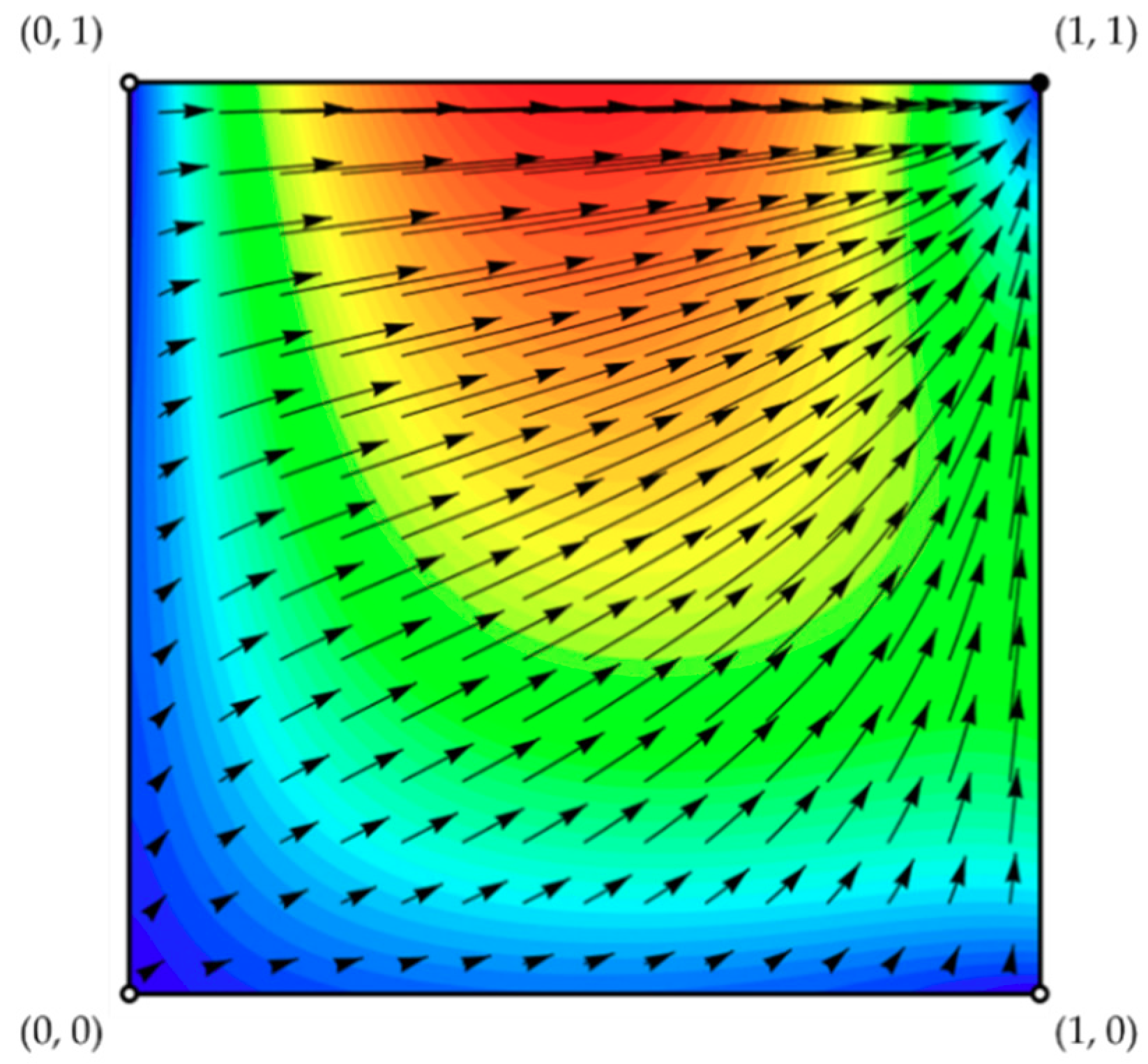
The phase diagram which was created using Dynamo [41] is shown in Figure 9. The result illustrates the evolutionary process and how the system converges to a stable strategy.

In Figure 9, points represent the steady-states, in which black one represents the sable point and white points represent the unstable points. The colors in the phase diagram represent the speeds of motion under the dynamic: red is fast and blue is slow. The arrows show that the trajectories will converge to the steady-state (1, 1) no matter where the initial condition is. That indicates that the centralized strategy is evolutionarily stable from a long-term perspective. This result is corresponding to the propositions that are proposed in this paper.

4.3. Effects of Main Parameters

The effects of residual value $\Delta$, the environmental attention $\lambda$, environmental impact of remanufacturing process $e_r$, firm’s expected profit $L_m$ and $L_r$ on the tax and subsidy policies of government and pricing and return strategies of firms are studied in this section. Three values of $\Delta$, $\lambda$, $e_r$ and $\left(L_m, L_r\right)$ are considered to be interpreted as high, medium and low, respectively. The values are shown as follows:

$$\Delta \in \left\{15,10,5\right\},\lambda \in \left\{0.7,0.5,0.3\right\},e_r\in \left\{4,3,2\right\},\left(L_m,L_r\right)\in \left\{\left(0,0\right),\left(4300,2150\right),\left(4400,2200\right)\right\}.$$

The nonlinear optimization problems of the government model in different scenarios are solved with MATLAB R2014a.

4.3.1. Residual Value

The residual value is calculated by $\Delta =c_n-c_r$. Hence, the higher the residual value of remanufactured products, the lower the cost of remanufacturing processes, which means that products are more profitable. The results of the government model and the Stackelberg model with different values for $\Delta$ are listed in

Table 9. Government tax and subsidy policies $(\Delta )$.

$\mathbf{\Delta }$	$\mathit{t}$	$\mathit{s}$	$\overline{\mathit{E}\mathit{M}}$	$\overline{\mathit{E}\mathit{R}}$	$\mathit{E}\mathit{I}$	$\mathit{P}\mathit{R}$	$\mathit{x}$	$\mathit{y}$
15	37.3194	13.1639	4052.7609	2022.4316	38922.3878	128360.9928	1	1
10	37.1322	14.3977	3995.1923	1993.7034	45437.7166	127997.7544	1	1
5	36.9001	15.8391	3951.9661	1972.1324	51267.4796	127839.2082	1	1

and

Table 10. Pricing, return policies and profits of manufacturers and retailers $(\Delta )$.

$\mathbf{\Delta }$		${\mathit{\Pi }}_{\mathit{m}}^{*}$	${\mathit{\Pi }}_{\mathit{r}}^{*}$	${\mathit{p}}^{*}$	${\mathit{D}}^{*}$	${\mathit{\tau }}^{*}$
15	C	4052.7609	2022.4316	186.597	44.0209	0.6199
	M	2944.4723	1517.3707	262.2144	21.3357	0.30045
	R	2950.3691	1497.746	262.072	21.3784	0.16034
	N	2856.8884	1428.4442	264.3299	20.701	0
10	C	3995.1923	1993.7034	188.7794	43.3662	0.52902
	M	2926.0803	1496.4435	262.7065	21.188	0.25847
	R	2914.0878	1473.0707	262.996	21.1012	0.10551
	N	2860.765	1430.3825	264.2831	20.7151	0
5	C	3951.9661	1972.1324	190.4634	42.861	0.44659
	M	2913.0135	1480.6187	263.081	21.0757	0.2196
	R	2888.1448	1452.7173	263.6807	20.8958	0.052239
	N	2865.575	1432.7875	264.225	20.7325	0

.

We consider $\Delta \in \left\{15, 10, 5\right\}$ as high, medium and low profit remanufactured products, respectively. In Table 9, as the residual value of the remanufactured products decreases, the subsidy that is allocated to the manufacturers increases. By reducing the residual value from 15 to 5, the subsidy is raised from 13.1639 to 15.8391.

The reason is that firms have enough motivation to remanufacture when the residual value of used products is high. For low profit remanufactured products, the government allocates a higher subsidy to promote environmental preference. Although the government allocates a higher subsidy for the low-profit products, the return rates are still less than the return rates of high-profit products. Therefore, besides increasing the subsidy, it is also important to develop technology so that we can recycle more material from used products.

By considering the government regulations, our results are different from past literature. Savaskan et al. (2004) [7] found that in decentralized channels, it is the most effective that the retailer takes the charge of collection activity. Our results show that when residual values are low, the manufacturer can obtain more profit by directly collecting the used products from customers. The reason is that model M is more sensitive to the change of subsidy, has a higher return rate and eventually receives more subsidy from the government than model R. Therefore, manufacturers and retailers that adopt model M have higher profit than adopt model R.

From this example, we found that the government prefers to allocate subsidy to low profit remanufactured products.

4.3.2. Environmental Impact of Remanufacturing Process

Although the environmental impacts of the remanufacturing process are lower than the manufacturing process $\left(e_r\le e_n\right)$, the remanufacturing process still have environmental impacts. The effects of $e_r$ on decisions of government, manufacturers and retailers are illustrated by numerical experiments. The results of the government model and the Stackelberg model with different values for $e_r$ are listed in

Table 11. Government tax and subsidy policies $\left(e_r\right)$.

${\mathit{e}}_{\mathit{r}}$	$\mathit{t}$	$\mathit{s}$	$\overline{\mathit{E}\mathit{M}}$	$\overline{\mathit{E}\mathit{R}}$	$\mathit{E}\mathit{I}$	$\mathit{P}\mathit{R}$	$\mathit{x}$	$\mathit{y}$
2	37.3194	13.1639	4052.7609	2022.4316	38922.3878	128360.9928	1	1
3	37.5252	11.7222	4021.3445	2006.754	44023.7277	134104.498	1	1
4	37.7118	10.3245	3992.8874	1992.5532	48647.6095	139130.3496	1	1

and

Table 12. Pricing, return policies and profits of manufacturers and retailers $\left(e_r\right)$.

${\mathit{e}}_{\mathit{r}}$		${\mathit{\Pi }}_{\mathit{m}}^{*}$	${\mathit{\Pi }}_{\mathit{r}}^{*}$	${\mathit{p}}^{*}$	${\mathit{D}}^{*}$	${\mathit{\tau }}^{*}$
2	C	4052.7609	2022.4316	186.597	44.0209	0.6199
	M	2944.4723	1517.3707	262.2144	21.3357	0.30045
	R	2950.3691	1497.746	262.072	21.3784	0.16034
	N	2856.8884	1428.4442	264.3299	20.701	0
3	C	4021.3445	2006.754	187.6258	43.7123	0.58404
	M	2931.1188	1505.8837	262.4841	21.2548	0.28399
	R	2941.0448	1490.5159	262.2442	21.3267	0.15995
	N	2852.6297	1426.3149	264.3813	20.6856	0
4	C	3992.8874	1992.5532	188.559	43.4323	0.54995
	M	2918.9721	1495.4515	262.7299	21.181	0.2682
	R	2932.3129	1483.6853	262.4073	21.2778	0.15958
	N	2848.7711	1424.3856	264.428	20.6716	0

.

By increasing the environmental impact of remanufactured products, the subsidy is decreased. That means that the government is more willing to support the low-pollution, low-consumption remanufactured products. In practice, governments also have the same behaviors that promote products that have better environmental preferences. For example, in China, the government promotes green home appliances by introducing subsidy with proposed subsidies of CNY 26.5 billion [42].

Moreover, as shown in Table 11, the remanufactured products that have low environmental impacts receive more subsidy which leads to the increase of return rates.

4.3.3. Environmental Attention

The government needs to consider the trade-off between public revenue and environmental issues. We set different values for environmental attention to illustrate the situations when the government pays different attention to environmental issues. The results of the government model and the Stackelberg model with different values for $\lambda$ are listed in

Table 13. Government tax and subsidy policies $\left(\lambda \right)$.

$\mathit{\lambda }$	$\mathit{t}$	$\mathit{s}$	$\overline{\mathit{E}\mathit{M}}$	$\overline{\mathit{E}\mathit{R}}$	$\mathit{E}\mathit{I}$	$\mathit{P}\mathit{R}$	$\mathit{x}$	$\mathit{y}$
0.7	37.3194	13.1639	4052.7609	2022.4316	38922.3878	128360.9928	1	1
0.5	38.6123	1.6358	3856.0727	1924.2791	57649.4867	160077.2693	1	1
0.3	38.7356	0	3837.4026	1914.9622	60096.3688	162289.2505	1	1

and

Table 14. Pricing, return policies and profits of manufacturers and retailers $\left(\lambda \right)$.

$\mathit{\lambda }$		${\mathit{\Pi }}_{\mathit{m}}^{*}$	${\mathit{\Pi }}_{\mathit{r}}^{*}$	${\mathit{p}}^{*}$	${\mathit{D}}^{*}$	${\mathit{\tau }}^{*}$
0.7	C	4052.7609	2022.4316	186.597	44.0209	0.6199
	M	2944.4723	1517.3707	262.2144	21.3357	0.30045
	R	2950.3691	1497.746	262.072	21.3784	0.16034
	N	2856.8884	1428.4442	264.3299	20.701	0
0.5	C	3856.0727	1924.2791	193.0613	42.0816	0.35003
	M	2859.8668	1444.929	263.9328	20.8202	0.17318
	R	2884.1647	1444.7868	263.3432	20.997	0.15748
	N	2830.1867	1415.0934	264.6531	20.6041	0
0.3	C	3837.4026	1914.9622	193.6778	41.8967	0.31422
	M	2851.7081	1437.9871	264.0997	20.7701	0.15578
	R	2876.1824	1438.0912	263.5056	20.9483	0.15711
	N	2827.6468	1413.8234	264.6839	20.5948	0

.

As shown in Table 13, the subsidy policy is very sensitive to the environmental attention of the government. When the government pays a low attention to the environmental issues $\left(\lambda =0.3\right)$, no subsidy will be allocated to the remanufactured products. By increasing $\lambda$, the government will allocate more subsidies to the manufacturers. When $\lambda =0.7$, the subsidy is raised to 13.1639. Observing Table 13 and Table 14, as $\lambda$ decreases, the retail prices increase, which leads to a decrease in return rates and total demand, and eventually, the profits of retailers and manufacturers decrease.

4.3.4. Firm’s Expected Profit

In the previous examples, we set $L_m=0$ and $L_r=0$, which means that the manufacturers and retailers are willing to enter the market as long as they don’t lose money. The result is that the government collects a relatively higher tax from the firm in all the examples. Here, we consider that the manufacturers and retailers are willing to enter the market only when the average profit is high enough. The results of the government model and the Stackelberg model with different values for $L_m$ and $L_r$ are listed in

Table 15. Government tax and subsidy policies $\left(L_m,L_r\right)$.

$\left({\mathit{L}}_{\mathit{m}},{\mathit{L}}_{\mathit{r}}\right)$	$\mathit{t}$	$\mathit{s}$	$\overline{\mathit{E}\mathit{M}}$	$\overline{\mathit{E}\mathit{R}}$	$\mathit{E}\mathit{I}$	$\mathit{P}\mathit{R}$	$\mathit{x}$	$\mathit{y}$
(0,0)	37.3194	13.1639	4052.7609	2022.4316	38922.3878	128360.9928	1	1
(4300,2150)	32.1401	18.0214	4308.3963	2150.0002	29161.1693	84852.9481	1	1
(4400,2200)	28.7592	17.8515	4408.5922	2200.0005	29110.9354	70319.6556	1	1

and

Table 16. Pricing, return policies and profits of manufacturers and retailers $\left(L_m,L_r\right)$.

$\left({\mathit{L}}_{\mathit{m}},{\mathit{L}}_{\mathit{r}}\right)$		${\mathit{\Pi }}_{\mathit{m}}^{*}$	${\mathit{\Pi }}_{\mathit{r}}^{*}$	${\mathit{p}}^{*}$	${\mathit{D}}^{*}$	${\mathit{\tau }}^{*}$
(0,0)	C	4052.7609	2022.4316	186.597	44.0209	0.6199
	M	2944.4723	1517.3707	262.2144	21.3357	0.30045
	R	2950.3691	1497.746	262.072	21.3784	0.16034
	N	2856.8884	1428.4442	264.3299	20.701	0
(4300,2150)	C	4308.3963	2150.0002	180.2145	45.9356	0.75843
	M	3091.5253	1611.6644	260.0379	21.9886	0.36305
	R	3079.5123	1572.1777	260.3227	21.9032	0.16427
	N	2965.1113	1482.5556	263.035	21.0895	0
(4400,2200)	C	4408.5922	2200.0005	178.515	46.4455	0.7629
	M	3164.9286	1649.2091	259.1891	22.2433	0.36536
	R	3153.384	1609.5718	259.4596	22.1621	0.16622
	N	3036.8414	1518.4207	262.1898	21.3431	0

.

When we set $L_m=4300$ and $L_r=2150$, the government increases the subsidy from 13.1639 to 18.0214 and also decreases the tax from 37.3194 to 32.1401 to make the manufacturers and retailers willing to enter the market. According to those results, the expected revenues of the manufacturer and retailer are satisfied. We found that the policy can increase the return rate up to 0.75843 in the centralized model and the rates are slightly increased in model M and model R. In this example, the centralized supply chain is more sensitive to the tax and subsidy policy. Also, with higher subsidy and lower tax, the profits of manufacturers and retailers in all channel structures are increased. However, the subsidy is decreased slightly from 18.0214 to 17.8515 when we continually increase the expected profits of the manufacturers and retailers. The reason is that in this model, the government reallocates the subsidy which comes from tax. Therefore, when tax is decreased, the subsidy that the government can allocate will also be reduced.

5. Discussion

The results from the numerical experiments show that tax and subsidy policies play an important role in a closed-loop supply chain that influences the pricing and investment decisions of firms. The centralized supply chain model is preferred for the government and it is also chosen by the market. Considering the balance between public revenue and environmental issues, the government’s best policy is to allocate a high subsidy to low-pollution and low-profit remanufactured products.

The tax and subsidy have complex impacts on demands and return rates in a dynamic closed-loop supply chain. Firstly, we analyze the influence of tax. By conducting the numerical experiments, we find that the higher the tax, the lower the return rate. The reason is that the collectors need to invest a lot of money to promote the return rate in this model. When the government increases the tax on new products, the total profits of the manufacturers and retailers decrease. As a result, to keep their profits, the best strategy for them is to decrease the investment for the return rate. Therefore, high tax leads to a low return rate and low total demand.

Secondly, we illustrate the influence of subsidy. By increasing the subsidy to the remanufactured products, both the demands of remanufactured products and return rates are increased in model C and M. Model C is more sensitive than model M which means that the subsidy is more “effective” in model C. However, models R and N are not sensitive to the change of subsidy. Because of the centralized structure, manufacturers and retailers should share their information to make an integrated decision. By the integrated channel, manufacturers and retailers are willing to make more investment in return rate compared with model M. In our model, the subsidy is allocated to the manufacturer. In the decentralized model R, to maximize their own profits, the manufacture’s best strategy is to keep the subsidy instead of sharing it with the retailer who is in charge of collecting the used products. In model N, the return rate keeps at 0, because manufacturers and retailers do not recycle the products. We suggest that the government should be careful with the high tax, because it may lead to bad influences on the market demand and remanufacturing industry. Because centralized supply chains are more sensitive than decentralized ones, the government should allocate the subsidy to the manufacturers that have good cooperation relationship with their upstream or downstream partners. The government should also have a sound allocation system to make sure that the allocation is spent on remanufacturing.

Thirdly, by analyzing the evolutionary dynamics, we find that the centralized structure is more competitive in the market than decentralized ones. The results show that in the centralized structure the products are sold at a lower price. Therefore, they have more market demand. The centralized supply chain is always preferred in the market because of those natures.

Finally, the effects of several main parameters on the decisions of the government, manufacturers and retailers are analyzed. The results show that low-pollution and low-profit remanufactured products are worth allocating a high subsidy to. The reason is that the firms want to maximize their profit in the competition. Although the remanufactured products have low pollution, the firms will not promote remanufacturing when the products have a low profit. By allocating a high subsidy to these products, the government could improve the environmental performance of society. For the high-profit products, the firms have enough motivation to remanufacture the used products. Therefore, the government does not need to allocate high subsidy to this type of products.

6. Managerial Insights

The resulting managerial insights indicate that when the government increases the tax, both return rate and demand for new products are decreased. The reason is that higher tax leads to lower investment to return rate and lower total market demand. By allocating subsidies to the remanufactured products, both return rates and demand for remanufactured products are increased in model C and model M. Also, subsidy policy is more successful in model C. By contrast, a subsidy is not effective in model R and model N. This is because in model R the subsidy for remanufactured products are allocated to the manufacturers, and to optimal their own profits, the subsidy is not transferred to the retailers. The stability of each structure is investigated. We have found that the centralized closed-loop supply chain is always preferred in the market because the cooperation leads to low retail price, high demand and high profits. Also, the centralized structure is preferred for the government because the manufacturers and retailers are sensitive to the government policies and have high return rate. Numerical experiments in different scenarios have shown that the low pollution, high profit remanufactured products are worth allocating subsidy to. When we set a lower bound of the firm’s revenue, the government will increase the subsidy and decrease the tax.

7. Conclusions

In this paper, we have focused on the government tax and subsidy policies in closed-loop supply chains. In the local markets, four supply chain structures have been considered and the optimal wholesale price, retail price and return rate are obtained for each structure based on the Stackelberg model. To describe the whole market, an evolutionary game model has been adopted. Furthermore, we have provided proofs that the centralized structure is the evolutionarily stable strategy. Then, a government model has been developed to obtain the optimal tax and subsidy policies considering both environmental issues and public revenue. Finally, numerical experiments have been conducted to illustrate the proposed model.

There are several future research directions. First, we assumed that demand is a linear function of the retail price. Further research might explore other demand functions, for example, the non-linear function. Second, the manufacturer is considered to be the supply chain leader and the retailer is the follower. A further study could investigate the effects of leadership structure in this model. Third, the perfect substitution between new products and remanufactured products is considered in this paper. In a future study, it would be interesting to consider the substitutability concept in the closed-loop supply chain by developing a new demand function. Fourth, in the proposed model, the government has only one possible policy toward different channel structures. More flexible tax and subsidy policies can be considered in future studies. Furthermore, the return rate is a function of investment in this paper. Further research could allow the return rate to be affected by other factors. Finally, the third party plays an increasingly important role in reverse logistics. Therefore, the model can be extended to third-party scenarios.