Article

Designing a New Shuttle Service to Meet Large-Scale Instantaneous Peak Demands for Passenger Transportation in a Metropolitan Context: A Green, Low-Cost Mass Transport Option

School of Traffic and Transportation, Beijing Jiaotong University, No. 3 Shang Yuan Cun, Hai Dian District, Beijing 100044, China
*
Author to whom correspondence should be addressed.
Sustainability 2019, 11(18), 5025; https://doi.org/10.3390/su11185025
Submission received: 8 August 2019 / Revised: 1 September 2019 / Accepted: 10 September 2019 / Published: 13 September 2019
(This article belongs to the Section Sustainable Transportation)

Abstract

:
Currently, the green, sustainable development of metropolises is hindered by problems caused by Large-scale Instantaneous Peak-demands for Passenger-transportation (LIPP), such as traffic congestion and air pollution. To mitigate these problems, we propose a new type of demand-responsive service as an alternative to inefficient “door-to-door” service. The proposed service is based on service units designed to aggregate passengers for shuttle service. To guarantee service quality and efficiency, a maximum passenger walking time constraint, a request rejection mechanism and a scheme for ensuring solution feasibility are considered. Through numerical experiments, we prove the following: (i) the proposed transport option exhibits better performance (by 40.37% for passengers and by 35.79% for operators) than the door-to-door transport option for solving real cases. (ii) By testing different datasets, we prove that the proposed service is more suitable for the request distributions that are spatiotemporally concentrated. (iii) Regarding the individual components of the proposed clustering-first, routing-second solution framework, the proposed soft clustering algorithm exhibits better performance than the classical hard clustering method (by 8%), and the proposed routing algorithm is 1.5 times more efficient than the commercial solution software GAMS.

1. Introduction

1.1. Background

As very common phenomena in the development of metropolises, Large-scale Instantaneous Peak-demands for Passenger-transportation (LIPP) have led to a number of problems related to mobility management and environmental concerns, such as traffic congestion, air pollution, and traffic accidents [1,2,3]. These phenomena are of great concern to the managers of metropolises because of the characteristics of the corresponding demands. These characteristics are markedly different from those of the transportation demands in general cities in the following ways.
(i) The peak demands in metropolises are unpredictable and instantaneous. Multiple sources (e.g., commuters and tourism traffic) and many factors (e.g., weather [4], festivals and special events) can cause demands to fluctuate irregularly and without warning.
(ii) The high population densities and clear boundaries of urban functional areas result in peak demands with certain spatiotemporal similarities in terms of origins and destinations (e.g., demands of commuters who live in the same residential areas and work in the same business districts).
This study is motivated by the desire to seek a new type of demand-responsive service, called large-scale instantaneous-peak-demand-responsive express shuttle service (LIPDRS), that can accommodate the LIPP of a metropolis, while balancing the benefits to operators and passengers. As an alternative to “door-to-door” transportation or frequency services, LIPDRS requires passengers to gather at certain locations, from which they are served by shuttles. Therefore, the LIDPRS design process involves first assigning passengers to certain service units and then transporting them along certain routes. LIPDRS has the advantages of a large capacity (ability to accommodate occasional massive demands), high flexibility (planning based on dynamic phone/Internet requests), low cost (affordability for passengers) and an acceptable level of convenience (passengers are required to gather at certain locations to be served in accordance with their requests). With these advantages, LIPDRS is an innovative means of increasing accessibility between high-circulation areas in a metropolis, such as residential districts and central business districts. As a complement to passenger transit systems, LIPDRS can help solve mobility and accessibility problems in a metropolitan context. In addition, this new transport option can encourage people to reduce their proportions of travel by private cars and thus reduce the cost of and pollution due to urban transportation, thereby improving the sustainability of metropolitan development.
However, the realization of LIPDRS comes at the cost of additional complexity. Since passengers are required to gather at certain locations for service, certain challenges arise that must be solved to make LIPDRS possible. These challenges are as follows:
(i) For a fully coordinated transportation service, involving large numbers of passengers and vehicles, the resulting optimization problem needs to be addressed using a holistic approach enabling the joint determination of the vehicle service locations, service time windows, routes, and passenger-to-vehicle assignments subject to rather restrictive travel demand requests. [5]
(ii) The service must strike a suitable balance between operator profitability and passenger convenience/accessibility. The balance among efficiency, effectiveness and equity of service is a key concern in the LIPDRS design process. It is clear that a demand-responsive transportation service does not need to serve all received requests if doing so will result in inefficiency. However, the problem of how to design an appropriate rejection strategy then arises, and the criteria for rejection are difficult to determine. [6]
(iii) Unlike a general demand-responsive bus service, LIPDRS abandons the door-to-door service model. Two additional major challenges that consequently arise are whether the requesters can accept this change and how to describe the threshold for passenger acceptance of LIPDRS from a general cost perspective.
(iv) The relevant control parameters, such as the optimal number of service locations, are difficult to determine [7].
(v) It must be possible to solve real-scale problems using the developed approach.
In this study, we build a mixed-integer programming model with dual objectives to optimize the service from the perspectives of both passengers and operators, following the principle of clustering first, routing second, to solve the LIPDRS design problem. The contributions of this study are four-fold:
(i) We propose a new transport option along with a complete system of modeling and solution methods. A maximum passenger walking time constraint, a request rejection mechanism and a scheme for ensuring solution feasibility are all considered in this scheduling system.
(ii) The proposed transport option is proven to achieve better performance (by 40.37% for passengers and by 35.79% for operators) than the door-to-door transport option when faced with real-world demands.
(iii) By testing on different datasets, we prove that the proposed service is more suitable for the request distributions that are spatiotemporally concentrated. We find that when the ratio of requests that are spatiotemporally concentrated is greater than 50%, LIPDRS is the more suitable option.
(iv) The performance advantages of the proposed clustering-first, routing-second solution framework are proven through experiments. Regarding the individual components of this framework, the proposed soft clustering algorithm is proven to be superior to the k-means hard clustering method (by 8%), and the proposed routing algorithm is proven to be 1.5 times more efficient than the commercial solution software GAMS.

1.2. Literature Review

Demand-responsive services are an important means of coping with special passenger demands. Existing passenger transportation systems include demand-responsive services such as customized buses and dial-a-ride services [8]. However, among the existing public transport options, neither door-to-door services (e.g., dial-a-ride services or carpooling) nor frequency services (e.g., customized buses) can accommodate LIPP; the existing methods face problems of capacity (insufficient vehicles), efficiency (too many boarding and alighting actions [9]) and quality (e.g., overcrowding and excessive waiting intervals [10]). We present a detailed comparison of LIPDRS with other urban public transport options in Table 1. By listing the main features (including schedule frequency, target demand, decision basis, request method, service locations, price and convenience) of each transport options, we find that none of the classical services can accommodate the characteristic of LIPP (the peak demands in metropolises are unpredictable and instantaneous). Taxis do not offer prescheduling before operating, and their decisions are based on the driver, making taxis limited and uncertain. Additionally, taxis do not offer advantages in terms of price. Thus, they can meet occasional individual demands but not LIPP. The other options with detailed scheduling also cannot accommodate the LIPP. School buses need to guarantee the safety of students, so their decisions are based on registered information from schools, and they travel between homes and schools directly along fixed routes. Conventional shuttles focus on serving passengers with related fixed travel demands, and they have poor adaptability to instantaneous peak demands. Although dial-a-ride services and car-sharing services are responsive to flexible demands, their capabilities are limited, and they cannot reduce the number of cars on the road network; thus, they cannot meet the demand for transporting mass passengers. Moreover, the prices of these two options of transportation are relatively high. Comparing these methods reveals that it is necessary to propose new transportation options.
Regarding methodologies, combinations of request clustering and routing methods based on geographical similarities have been the focus of existing research. Cullen et al. [28] proposed a clustering-first, routing-second heuristic model. Bodin and Sexton [29] also constructed a clustering-first, routing-second heuristic model for the pickup and delivery problem with time windows (PDPTW). In this model, passengers are first partitioned into clusters. Then, the clusters are assigned to routes using the algorithm developed by Sexton and Bodin [30,31]. Finally, the algorithm swaps passengers between routes for route re-optimization. Dumas et al. [6] introduced the concept of mini-clusters, in which passengers with high spatiotemporal proximity are clustered together. In this algorithm, a heuristic method is used to produce a set of mini-clusters. Then, a column generation (CG) algorithm is used to optimally combine the mini-clusters into vehicle routes. Finally, the algorithm performs route re-optimization to obtain the optimal schedule for each vehicle. Desrosiers et al. [32] proposed another approach to mini-cluster construction by means of a parallel insertion method based on the spatiotemporal proximity of the requests. Ioachim et al. [33] applied an optimization-based technique instead of a heuristic method for the construction of mini-clusters. In addition to these studies, Pankratz [34], Bard and Jarrah [35], Qu and Bard [36], and Masson et al. [37] also applied clustering algorithms for the PDPTW. The results of these studies show that high-quality vehicle plans can be obtained only through the integrated consideration of clustering and routing.
In the field of operations research, a routing problem for demand-responsive service is typically formulated, as either a vehicle routing problem with time windows (VRPTW) [38,39] or a PDPTW [40,41]. In most VRPTWs or PDPTWs, the number of passengers served, the operating cost, and the service quality are the three major objectives to be optimized, either separately or simultaneously [42]. Typical vehicle-to-passenger matching and routing constraints include time window constraints, capacity constraints, coupling constraints, and maximum ride time constraints, which typically give rise to an NP-hard problem [43,44]. Many researchers have focused on studying corresponding solution techniques. CG algorithms [45,46], branch-and-price algorithms [15], branch-and-cut algorithms [47], branch-and-cut-and-price algorithms [48], tabu search algorithms [49], and dynamic-programming-based metaheuristics [14] can be used to solve problems of this type. The proposed LIPDRS problem can be regarded as an offline multivehicle routing problem because all the requests are assumed to be known beforehand.
Although significant improvements have been achieved in solving demand-responsive service design problems, LIPDRS design still poses several challenges, as discussed in Section 1.1. To overcome these challenges, we model the LIPDRS decision process using a mixed-integer programming model with dual objectives to optimize the service from the perspectives of both passengers and operators. This model includes a carefully designed passenger walking time constraint and request rejection mechanism to ensure that the resulting service plan can guarantee not only good quality of service, but also improved operational efficiency. Additionally, this paper proposes a clustering-first, routing-second framework for solving the proposed model. A modified version of the fuzzy c-means clustering algorithm and a CG algorithm are utilized in this framework to determine the service units and perform vehicle assignment and routing, respectively. In addition, to overcome the challenges caused by relaxing the model variables, a branching scheme is proposed.
The rest of the paper is organized as follows. Section 2, presents details of the methodology for solving the LIPDRS design model, including the (first) clustering phase, i.e., the determination of service units (DSU), and the (second) routing phase, i.e., fleet assignment and routing (FAR). Section 3 presents a numerical experiment conducted to analyze the performances of the proposed services on different request datasets. In addition, we present comparisons between the proposed LIPDRS option and the existing door-to-door transport option based on various artificial datasets to evaluate the application scope of our proposed method.

2. Methodology

In this section, the methodology of the present study is presented. We first introduce the whole architecture for LIPDRS design, including the overall service decision process and the construction of the LIPDRS design model (LIPPD). Second, we introduce the corresponding clustering-first, routing-second algorithm. Finally, we introduce the criteria for evaluating the results.

2.1. Framework for LIPDRS Design

2.1.1. Overall Service Decision Process

To enable an effective and feasible shuttle service, a seven-step process in which the requesters can be actively involved is designed, as shown in Figure 1.
  • Request Collection. Potential passengers submit their travel requests (each consisting of a preferred location tuple with boarding and alighting locations and a time window tuple with the expected boarding and alighting times) through mobile phones or other devices. The data collection and planning period is designated as one day; that is, in one day, the demands for the next day are collected and planned. Any request that is submitted before the deadline (either a specified moment, such as 12:00 p.m., or some specified number of hours ahead of the service time) will be pushed into the request pool to wait for stage 2. Other requests will be marked as overdue requests and will wait for stage 5.
  • Determination of Service Units (DSU). Requests in the request pool are aggregated into a set of service units (which specify the locations at which and time windows in which the requesters will be served) using the approach described in Section 2.3. The set of service units will be sent to the service pool to wait for stage 3. Isolated requests (i.e., requests that do not belong to any service unit) from the request pool are also detected in this stage. These isolated requests will wait for stage 4.
  • Fleet Assignment and Routing (FAR). Vehicles are assigned to specific service units, and the fleet is routed, subject to capacity constraints, spatiotemporal constraints, procedure constraints, etc. Through this process, the operators obtain the service routes and scheduled service plan (timetable) for the LIPDRS.
  • Economic Evaluation. The operators use evaluation metrics to compare the generated plan with other transport options and evaluate whether the plan will be economically acceptable to passengers. These evaluation metrics are discussed in Section 2.5.
  • Request Rejection. To ensure the quality and efficiency of demand-responsive transport, reasonable rejection of certain transport requests is an integral part of designing a transport plan. Three types of requests need to be rejected according to different rejection rules: overdue requests, isolated requests, and uneconomical requests. These three types of rejection occur in different parts of the planning process, as shown in Figure 1. The specific rejection mechanism will be discussed in Section 2.
  • Information Feedback. This stage consists of two parts: feedback to requesters who have been assigned to service units, with scheduled boarding and alighting information, and feedback to rejected requesters.
  • Service Implementation. After receiving their feedback information, passengers will walk or bike to their specified boarding locations within their specified time windows for service.

2.1.2. LIPDRS Design Model (LIPPD)

The main idea on which the formulation of the LIPPD is based is that it is necessary to first determine service units based on the received requests and then assign and route the fleet in accordance with those service units. We formally formulate the LIPPD as follows:
Objectives:
Minimize   k M ( i V D e j V D e c i j x i j k + F j V x D e + j k ) + i N P ( 1 k M z i k )
Maximum   L ( c ) = j = 0 n 1 i = 0 c 1 u j i m | | r ¯ v i | | 2 / ( c 1 ) j = 0 n 1 i = 0 c 1 u j i m | | r j v i | | 2 / ( n c )
subject to
| | r j v i | | W A t m w t ( i N , v i S , r j R )
v i C a d = { v j | 0 j < c }
k M z i k 1 ( i N )
j V D e x l j k = j V D e x j l k = z i k ( i N , l V , k   M )
j V D e x D e + j k 1 ( k M )
i V D e + x i D e k 1 ( k M )
j V D e x D e + j k = i V D e + x i D e k ( k M )
e i D i l i ( i V D e )
D i + D i ( i N )
x i j k = 1 D i + t i j + o p j D j ( i , j V D e + , k M )
x i D e k = 1 D i + t i D e + o p D e l D e ( i N , k M )
y D e + = 0
y l k M Q z i k ( i N , l V )
x i j k = 1 y i + q i y j ( i , j V D e , k M )
i V , j V x i j k d i j d m a x ( k M )
i V , j V x i j k t i j t m a x ( k M )
u j i   ( j = 1 c 1 u j i = 1 ,   0 u j i 1 )  
x i j k { 0 , 1 } ( i , j V D e , k M )   and   z i k { 0 , 1 } ( i N , k M )
D i 0 ( i V D e )   and   y i 0 ( i V D e )
The related objective functions, constraints, variables, sets and parameters are defined as follows.
• Objective Functions
Equation (1a) represents the cost of operation, including the fixed and variable costs of using vehicles and the penalties for the cancelation (rejection) of service units. A smaller objective function value is better. Equation (1b) guides the DSU process. Unlike in the case of taxi and door-to-door services, LIPDRS requesters will be served at specified boarding/alighting locations (i.e., the locations of the service units) instead of the requesters’ home/work locations [50]. The number of service units impacts the efficiency, effectiveness and equity of passenger service and vehicle operation. If the service units are too densely distributed (meaning that the clusters are small in size), the speed of service will not be effectively accelerated; if the service units are too sparsely distributed, more requesters will have to walk farther. Therefore, we select the ratio between compactness and divergence as one of the objective functions of the LIPPD, where (a) the divergence drives the distances between service units to be as large as possible and (b) the compactness drives the walking distances (times) between requesters and service units to be as small as possible. In this case, a larger objective function value is better. To extend the problem considered in this paper to other fields, different objective functions can be chosen from existing studies [7,51,52].
• Constraints
Equation (2) is a spatiotemporal constraint, namely, a maximum walking time constraint, where m w t denotes the maximum walking time; the norm · W A t will be explained in Section 2.2.2. For example, in Figure 2, there are 17 requests and 6 candidate service units. As a result of the DSU process, 2 of the candidate service units are selected, and the 17 requests are grouped into service unit 2 and service unit 5. Within each service unit, the time windows for boarding and alighting satisfy the intracluster operation time constraint. Service unit 2 consists of 14 close requests, and the walking time between each requester and the service location is less than the predefined maximum walking time m w t . Equation (3) ensures that the service units are selected from among the candidate service units because the vehicles should not park at arbitrary locations. Equation (4) ensures that each service unit is assigned to exactly one vehicle or is canceled. Equation (5) enforces that a vehicle must visit both the boarding and alighting points of every service unit assigned to it. Equations (6)–(8) ensure that the vehicles either perform assigned tasks or remain idle. Equations (9)-(12) together form the precedence constraints. Equations (13)–(15) together form the capacity constraints. Equations (16) and (17) represent the maximum distance constraint and the maximum driving time constraint, respectively.
• Decision Variables
The variables of this model are as follows.   x i j k ( ( i , j ) ( V × V ) · { ( D e + , j ) | j V } · { ( j , D e ) | j V } , k M ) is a binary variable that is equal to 1 if vehicle k is scheduled to travel from location i to location j and is equal to 0 otherwise. z i k ( i N , k M ) is a binary variable that is equal to 1 if service unit i is assigned to vehicle k and is otherwise equal to 0. c , a positive integer variable, represents the number of clusters (i.e., the number of service units). The u j i ( j = 1 c 1 u j i = 1 , 0 u j i 1 ) are positive variables. U n × c is the matrix of membership values, and u j i U n × c is the membership value of the j t h request with respect to service unit i . D i ( i V D e ) is an integer variable that specifies the departure time at vertex i . y i ( i V D e ) is an integer variable that specifies the load of the vehicle when arriving at vertex i . We define q D e + = 0 for all k M .
• Sets
In this model, N denotes the set of service units. For each service unit i N , a request group of size q i needs to be transported from boarding point i + to alighting point i . It is known that q i = q i + = q i , where positive quantities correspond to pickups and negative quantities correspond to dropoffs. We define N + { i + | i N } as the set of boarding points and N { i | i N } as the set of alighting points. Let V N + N . Furthermore, M represents the set of vehicles. Each vehicle k M has a capacity Q , a starting location D e + , and an ending location D e . We set D e D e + D e .
• Parameters
For all i , j V D e , c i j denotes the travel cost. F represents the fixed cost of a vehicle, and P represents the penalty for cancelling serving a service unit. Then, m is a fuzzifier with a value greater than 1, where a higher value indicates a higher degree of ambiguity [51]. n is the number of requests. r ¯ represents the average of the spatiotemporal features of all requests. r j represents the spatiotemporal features of the j t h request, and v i represents the spatiotemporal features of service unit i . These spatiotemporal features consist of location and time window information. We represent a request as an eight-dimensional vector r j = ( l o j + , t w j + , l o j , t w j ) = ( l n g j + , l a t j + , e j + , l j + , l n g j , l a t j , e j , l j ) , where ‘ + ’ indicates features corresponding to the origin and ‘ ‘ indicates features corresponding to the destination. Similarly, each service unit is associated with an eight-dimensional feature vector of the same form, v i = ( l o i + , t w i + , l o i , t w i ) = ( l n g i + , l a t i + , e i + , l i + , l n g i , l a t i , e i , l i ) , where ‘ + ’ indicates boarding information and ‘ ‘ indicates alighting information. Each candidate service unit is similarly represented in the form v i = ( l o i + , t w i + , l o i , t w i ) = ( l n g i + , l a t i + , e i + , l i + , l n g i , l a t i , e i , l i ) . The m w t denotes the maximum walking time. Then, we denote the set of requests by R = { r j | 0 j < n } , the set of service units by S = { v i | 0 i < c } (where c is the number of service units) and the set of candidate service units by C a d = { v i | 0 i < c } , where n , c and c are the numbers of elements of S , R and C a d , respectively. [ e i , l i ] denotes the time window, and o p i denotes the operation time. For all i , j V D e , d i j denotes the travel distance, and t i j denotes the travel time. For each service unit i N , the number of requests q i is given. Q is the capacity of vehicle. Additionally, each vehicle has an operation distance range [ 0 , d m a x ] and an operation time range [ 0 , t m a x ] (representing the driver’s working time).
Based on the description given in Figure 2, we further illustrate the model by means of a simple example of the LIPDRS design process. Objective function (1.2) and constraints (2) and (3) are used to select service units from among the candidate service units and assign requests to them in accordance with the spatiotemporal features of the requests. The bottom of Figure 2 shows the process of selecting service units. In this example, the requesters submit requests that contain spatiotemporal origin and destination information, represented by oblique-textured and cross-textured circles, respectively. The candidate service units are represented by untextured squares. Ultimately, two service units are selected, represented by textured squares; they are identified as service unit 2 and service unit 5. These two service units serve two branches of requests with different destinations. Each service unit has two components: the boarding component (oblique-textured squares) and the alighting component (cross-textured squares). Both components contain the corresponding locations and time windows for the requesters and vehicles. Requesters walk to the boarding location indicated by the boarding component, are transported to the alighting location indicated by the alighting component, and then proceed to their destinations.
In this example, five service units are selected, and the operator assigns them to vehicles in the fleet and designs routes for the fleet. Objective function (1.1) and constraints (3)-(20) are used for assignment and routing. Once the service routes have been determined, the fleet departs from the depot(s), visits each service unit within the corresponding service time window, and then returns to the depot. Generally, the LIPDRS solution comprises several service routes, such as the two example routes (0-1-1′-2-2′-0 and 0-4-5-4′-5′-3-3′-0) shown in Figure 2.

2.1.3. Clustering-First, Routing-Second Algorithm for Solving the LIPPD

The solution process for the LIPPD is the process of finding the optimal service units and service routes in accordance with the spatiotemporal features of the requests. Ideally, we wish to find an optimal solution to the LIPPD that considers the trade-off between passenger costs and vehicle costs [53]. However, from the model, we can see that it is not easy to obtain solutions to this problem: the objective functions are multitarget functions with nonlinear structures. Therefore, instead of looking for the globally optimal solution, we use a two-stage algorithm to find a near-optimal solution. This section introduces the clustering-first (DSU), routing-second (FAR) solution approach. This solution framework implies the following assumption about the priority of the targets: the burden placed on the passengers by this new service mode is minimized first, and the operational cost is then minimized. In other words, we pay more attention to the requesters’ costs than to the operators’ costs.
To facilitate clearer description throughout the rest of the paper, we use R M to denote the submodel comprising Equations (1a), (4)–(17), (19) and (20) and use C M to denote the submodel comprising Equations (1b), (2), (3) and (18). The DSU process focuses on solving C M , and the FAR process focuses on solving R M .

2.2. Preprocessing and Distance Measurement

2.2.1. Preprocessing

The preprocessing phase consists of two tasks: (i) the detection and deletion of self-contradictory requests and (ii) the detection and deletion of abnormal requests.
Since the service considered here needs to be feasible in an actual scenario, it is necessary to exclude user-submitted requests with self-contradictions. In general, such requests are not spatiotemporally feasible; for example, the separation between the expected time windows for boarding and alighting may be too small, meaning that a vehicle cannot complete the specified task, while obeying the speed limit in the corresponding road network. Such self-contradictory requests should be deleted to avoid infeasible solutions to the model. For this purpose, we use formula (21) to detect self-contradictory requests:
| | v i | | A m ς ,   v i C a d
where | | v i | | A m v i C a d is a norm defined as | | v i | | A m | | l i + , l i | | R l t ( e i e i + ) , with ς representing the operation time redundancy for a vehicle and a , b R l t representing the vehicle travel time (obtained from a digital map) between locations a and b . The definition of the norm | | a , b | | R l t will be discussed in Section 2.2.2.
In addition to self-contradictory requests, abnormal requests should also be detected and removed from the request pool. There are two main types of abnormal requests: (i) requests caused by misoperation, such as requests whose starting and ending locations are too close or repeated requests with the same ID number, and (ii) spatially invalid requests, such as requests corresponding to locations that are significantly beyond the scope of the service. The screening for such abnormal requests relies mainly on simple heuristic rules.

2.2.2. Distance Measurement

As a service operated in a metropolitan context, LIPDRS requires a reasonably accurate distance calculation method. The temporal and spatial distances between two points cannot be directly calculated using the Euclidean distance but should instead be calculated in accordance with the conditions of the road network, speed limits, etc. Measuring the distance by means of the path planning function of an electronic map is a viable option. Here, we define two temporal distance norms, | | ( l i + , l j + ) | | W l t and | | ( t w i , t w j ) | | t w t , and one spatial distance norm, | | ( l i + , l j + ) | | W l s , where | | ( l i + , l j + ) | | W l t and | | ( l i + , l j + ) | | W l s are obtained from a digital map (e.g., AMAP).
In addition, we define | | x i v j | | W A t as a measure of the temporal distance between a request and a service unit, as expressed by Equation (3). This measure is vitally important to the process of assigning requests to service units:
| | x i v j | | W A t = | | ( l i + , l j + ) | | W l t + | | ( t w i + , t w j + ) | | t w t + | | ( l i , l j ) | | W l t + | | ( t w i , t w j ) | | t w t
where | | ( a , b ) | | W l t represents the passenger walking time (obtained from a digital map) between locations a and b and | | ( a , b ) | | t w t represents the time difference between time windows a and b .

2.3. Clustering (First Stage): Determination of Service Units (DSUs)

2.3.1. Main DSU Flows

We introduce the DSU solution process in the form of the flow chart shown in Figure 3. During the DSU solution process, on one hand, the locations and time windows of the service units must be selected to allow the requests to be assigned to service units, and on the other hand, as in other clustering-based problems, determining the number of clusters c is also an important task [7]. Therefore, a cluster number determination method is required. To this end, the structure of this flow chart is composed of two loops and corresponding initialization modules. The outer loop is designed to determine the optimal number of service units, and the inner loop applies a clustering method to determine the service units in accordance with a given number of clusters.
In Figure 3, modules (3)–(7) compose the inner loop for the clustering task. The purpose of clustering, an unsupervised machine learning method, is to aggregate the requesters by generating centroids (which can be used as the basis for selecting service units) based on similarities among the spatiotemporal features of the requests. Among the many clustering methods available, we choose fuzzy c-means clustering (FCM) as the basic method of identifying service units and assigning requests. FCM is a soft clustering method. Unlike hard clustering methods (e.g., k-means), FCM simultaneously considers the possibilities that a data point may belong to multiple clusters by means of membership degrees, resulting in a much finer degree of data modeling that yields numerical results that can be used for further analysis [7]. However, the original FCM method cannot accommodate the walking time constraint, which is vitally important to our research. We therefore propose a new similarity measure to modify the original FCM to consider a limit on the walking time.
The outer loop, which is composed of the inner loop and modules (1), (2), (8) and (9), selects a number of candidate clusters from a set and passes this cluster number to the inner loop. This is an enumeration process. At the end of the loop, the number of clusters that results in the best objective function value is selected as the final number of service units. The number of service units impacts the efficiency, effectiveness and equity of passenger service and vehicle operation. If the service units are too densely distributed (meaning that the clusters are small in size), the speed of service will not be effectively accelerated; if the service units are too sparsely distributed, more requesters will have to walk farther. Thus, the number of service units is a key factor in striking this balance. We will introduce each module in detail throughout the rest of Section 2.3.

2.3.2. Initialization

There are two initialization modules in Figure 3. Module (1) is for the initialization of the set of the candidate numbers of clusters, c c , wherein we construct a set-in increments of one within a given range. The other initialization module is module (3). The elements in the matrix of membership values U n × c for FCM are randomly initialized in accordance with the following constraints: the elements u j i must satisfy j = 1 c 1 u j i = 1 and 0 u j i 1 .

2.3.3. Measurement of Similarity between a Request and a Service Unit

The norm for measuring the similarity of the j t h request to the centroid of cluster i is vitally important because it directly influences the objective function (1.2). In the flow of the DSU solution process, the similarities are calculated in module (5). A typical norm is the A-norm proposed by Bezdek et al. [54]. However, the A-norm can measure only geographical proximity and thus is not suitable for measuring spatiotemporal proximity, as is necessary for the walking time constraint. Therefore, we propose a Gaussian-kernel-based norm that allows the maximum walking time to be considered, as presented in (23):
| | r j v i | | W G A t = { | | r j v i | | W A t / e x p ( | | r j v i | | W 2 A t / 2 σ 2 ) , ( f o r   a n y   r j , v i : | | r j v i | | W A t m w t )     | | r j v i | | W A t   , ( f o r   a n y   r j , v i : | | r j v i | | W A t > m w t )
In (23), we use the temporal distance | | r j v x | | W A t to represent the distance between two locations instead of calculating the Euclidean distance. The definition of | | r j v x | | W A t can be found in Section 2.2.2.
A Gaussian kernel, a kernel type that is widely used in machine learning [55], can make objective function (1.2) valid only in a local area (i.e., if a requester’s walking time is greater than the maximum passenger walking time m w t , then the similarity to the corresponding service unit will be very low). However, as a result of the mechanism of generating the initial solution for FCM [7,56], the initially selected service units might be far away from any request. In other words, a service unit might have minimal similarity to all requests. Therefore, we design (23) as a piecewise function to avoid empty clusters (i.e., when there is at least one request in a service unit, the Gaussian kernel is used). In (23), σ is a width parameter that controls the range in the radial direction, whereby we can control m w t .

2.3.4. Iteration Method and Termination Criteria

In modules (4) and (6), the service units v i are reselected, and the membership values u j i are updated. For this purpose, we propose Equations (24) and (25). The norm a m C a d can be used to enumerate the candidate service units and find the nearest one to the centroid a i of the requests, where the centroid a i is calculated as a i = j = 0 n 1 ( u j i ) m r j / j = 0 n 1 ( u j i ) m .
u j i = 1 / s = 0 c 1 ( | r j v i | | r j v s | ) 1 m 1
v i = j = 0 n 1 ( u j i ) m x j / j = 0 n 1 ( u j i ) m m C a d
Following Bezdek [56], m = 2 is adopted in this study. Two criteria for terminating the iterative process are designed for module (7). One is a threshold ε . If | U p + 1 U p | < ε , then the iterative process terminates, where U p is the membership matrix in the p t h iteration. The other is a maximum number of iterations, m i . After either termination criterion is triggered, any remaining requests with very low similarities (close to 0) to any service unit become isolated requests.

2.4. Routing (Second Stage): Fleet Assigning and Routing (FAR)

We develop a model based on the pickup and delivery problem with time windows (PDPTW) for formulating the FAR problem. Considering the complexity of the search space in a large-scale network, we use a column generation (CG) algorithm in the framework for solving the model. In addition, to address the influence of variable relaxation, a branching scheme is used to generate a binary solution tree to enable the selection of a feasible and optimal solution.

2.4.1. Main FAR Flows

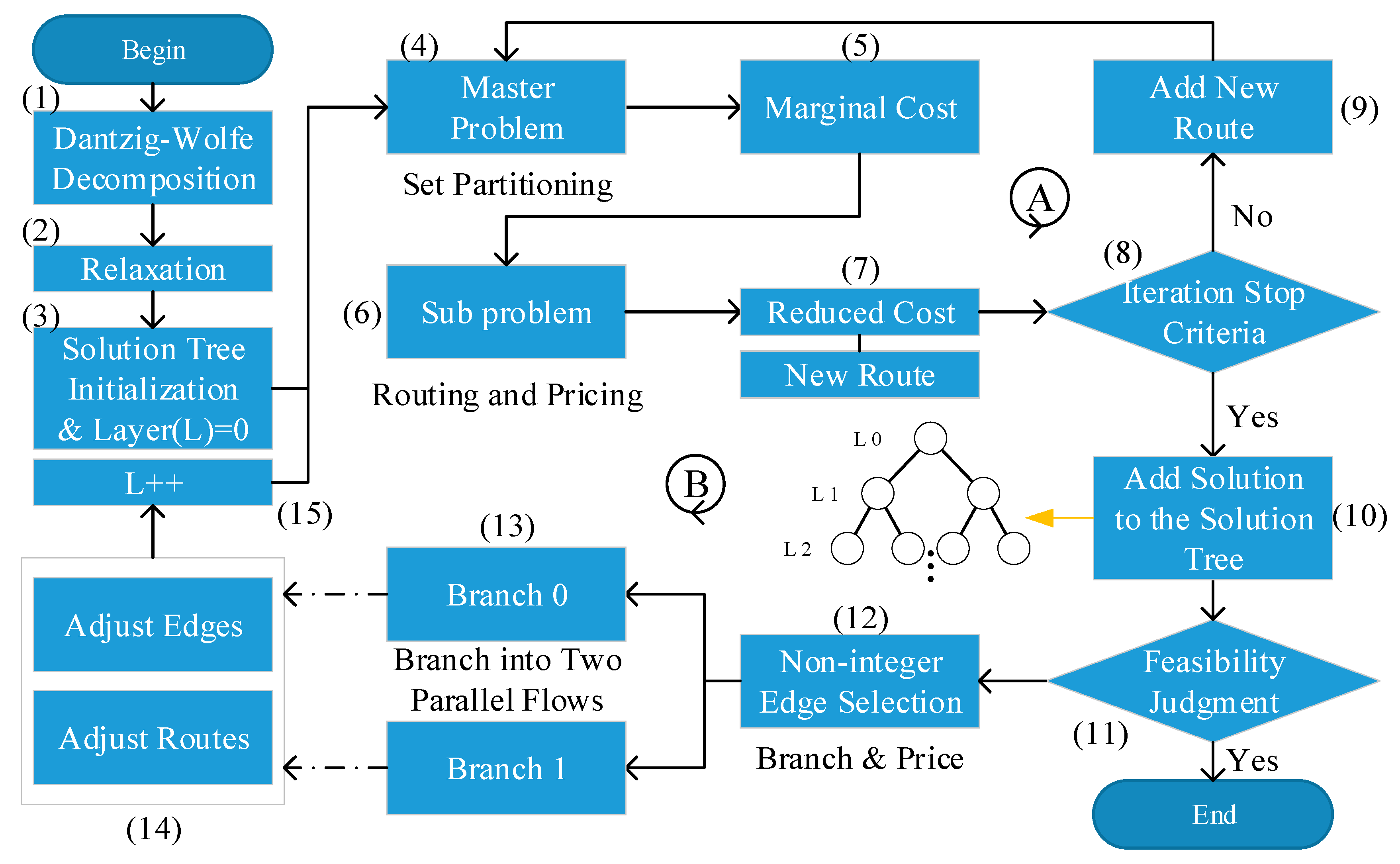
The FAR process converts the service units determined via the DSU process into service routes, which represent the specific times and order of the service units served by the fleet. We introduce the FAR solution process in the form of the flow chart shown in Figure 4. The structure of this flow chart is composed of two loops and corresponding initialization modules. These two loops are designed to calculate the model and to guarantee that there is no infeasible solution, namely, no noninteger solution, which can occur as a side effect of the relaxation of the model.
In Figure 4, the inner loop (denoted by A) applies the CG algorithm, iteratively solving the master problem and the subproblem. This loop is composed of modules (4)-(9). The outer loop (denoted by B) applies a branching scheme to avoid noninteger solutions. It is composed of loop A and modules (10)–(15). Modules (1)–(3) are the initialization modules for the two loops. Focusing on these two loops and the modules they include, we will elaborate on the details of the algorithm in Section 2.4.2, Section 2.4.3, Section 2.4.4, Section 2.4.5 and Section 2.4.6.

2.4.2. Initialization

(1)–(2): Dantzig-Wolfe Decomposition and Relaxation of the Master Problem
To circumvent the difficulties facing such large-scale problems [57], we decompose the model introduced in Section 2.1.2 via Dantzig-Wolfe (DW) decomposition. After DW decomposition, the original model has been decomposed into an equivalent combination of two smaller problems: a master problem (the fleet assignment problem) and a subproblem (the routing and pricing problem). The master problem is the set coverage problem, and the subproblem is the route planning and pricing problem. The decomposed model can be solved via a CG algorithm. To obtain the marginal cost of the master problem, we relax the integer decision variables of the master problem to positive variables.
(3): Solution Tree
A side effect of the relaxation of the master problem is that the route selection process may yield noninteger solutions. A mature approach for overcoming this problem of noninteger solutions is the branching approach [57]. To obtain information about when to start and end each branch, we design a solution tree with index L and a feasibility judgment method to store solutions and judge whether the process should terminate or continue.
As shown in Figure 4, the solution tree is a layered binary tree. The original solution is stored as the root. The feasibility judgment method is used only to judge the solutions in the L t h layer. If the feasibility judgment method detects that a noninteger route has been selected in the solution, then the branching method described in [57] is applied. Otherwise, no noninteger route has been selected in the solution, and the algorithm ends. Finally, we choose the best solution in the solution tree as the output.

2.4.3. Master Problem (Relaxed Set Partitioning Problem, MP)

The master problem M P is a set partitioning problem, which can be formulated as follows.
Objective:
Minimize   r k Ω c k θ k + i N P ( 1 r k Ω δ i k θ k ) = i N P + r k Ω θ k ( c k i N P δ i k )
subject to
r k Ω δ i k θ k 1 ( i N )
r k Ω θ k | M |
θ k [ 0 , 1 ] ( r k Ω )
Here, M denotes the set of available vehicles, Ω denotes the set of all feasible pickup and drop-off routes ( r k ) served by vehicle k , and c k denotes the cost of route r k .
The primary objective of M P is to minimize the number of vehicles needed, and the secondary objective is to minimize the total cost. Therefore, c k is calculated as c k = F C + V C L k , where L k denotes the length of route r k , V C denotes the unit cost of a vehicle, and F C denotes the fixed cost of a vehicle, which should be relatively large. This cost structure can be achieved by defining the travel costs c i j = d i j ( i D e ) and c D e j = F C + d D e j ( j D e ) .
Furthermore, let parameters δ i k be defined as follows:
δ i k { 1   i f   i N   i s   s e r v e d   o n   r o u t e   r k Ω , 0   o t h e r w i s e .
Let the θ k be positive variables of the master problem:
θ k [ 0 , 1 ]
If θ k = 1 , then route r k Ω is selected, and if θ k = 0 , then route r k Ω is not selected; otherwise, if θ k ( 0 , 1 ) , the solution is infeasible. The process of replacing the θ k with positive variables rather than integer variables is called relaxation, which is performed in module (2). Equation (27) ensures that each service unit will be either served or canceled, and the penalty for canceling service units is represented by i N P ( 1 r k Ω δ i k θ k ) in objective function (26). Equation (28) ensures that the number of selected routes cannot exceed the scale of the fleet.

2.4.4. Subproblem (Routing and Pricing Problem, S k )

Let the graph of the subproblem be denoted by G = ( N , E ) , and let the cost of each arc ( i , j ) E be denoted by c i j G . Then, the subproblem S k is formulated as follows:
Objective:
Minimize   i V j V c i j G x i j
subject to
j V x i + j = j V x j i + = z i ( i N )
j V x i j = j V x j i = z i ( i N )
j V x D e + j = 1
i V x i D e = 1
D i + D i ( i N )
D i + t i j D j + o p j + x i j M M ( i , j V D e + )
D i + t i D e l D e + o p D e + x i D e M M ( i N )
y D e = 0
y j y i q i + x i j M M ( i , j V )
y j y i q i x i j M M ( i , j V )
i V , j V x i j d i j d m a x
i V , j V x i j t i j t m a x
e i D i l i ( i V )
0 y i Q ( i V )
x i j { 0 , 1 } ( i , j V )
z i { 0 , 1 } ( i N )
The target of S k is to find routes that minimize the reduced cost for the master problem. In objective function (32), c i j G is composed of c i + j G c i + j P u i , c D e j G c D e j w and c i j G c i j ( i N + D e ), where u i and w belong to ( u , w ) , which is the marginal cost of the master problem M P .
In S k , the following variables are significant: z i ( i N ) , a binary variable, is equal to 1 if service unit i N is served by the vehicle and is equal to 0 otherwise. x i j ( ( i , j ) V × V ) , a binary variable, is equal to 1 if the vehicle travels from location i V to location j V and is equal to 0 otherwise. D i ( i V ) , an integer variable, denotes the departure time at location i V . y i ( i V ) , an integer variable, denotes the load of the vehicle when arriving at location i V .
Regarding the constraints, Equations (33) and (34) ensure that the vehicle visits either both the boarding and alighting points of a service unit or neither of them. Equations (35) and (36) ensure that the vehicle starts and ends at its depot. Equations (37)–(39) and (45) together form the precedence constraints. Equations (40)–(42) and (46) together form the capacity constraints. Equations (43) and (44) ensure that the vehicle will return within a limited travel distance and duration.

2.4.5. Iteration Termination Criteria

The solution process for M P and S k is embedded in loop A. After the input data and initial routes are obtained, M P is solved first, yielding a marginal cost ( u , w ) for S k . Then, S k is solved using a labeling method based on dynamic programming [58], and the solution is a new route for M P . The new route is the one that incurs the minimal reduced cost for M P . This process does not stop until the solution to S k meets the following termination criterion: the reduced cost of the returned route is equal to or greater than 0.
The individual termination criteria of the two loops are also important. In module (8), if the reduced cost obtained from the subproblem is greater than 0, then the loop stops. Otherwise, the loop continues. In module (11), if the solutions in the L t h layer are feasible, then the loop stops. Otherwise, the loop continues.

2.4.6. Branching Scheme

When a solution appears infeasible, namely, noninteger in nature, a branching scheme should be applied, as in modules (12)–(14). The rules of the branching scheme are as follows:
(i) For each arc ( i , j ) , calculate the values f i j = r k Ω b i j k θ k ( 0 f i j 1 , j b i j k = δ i k ( i , j N ) ) and select an arc that satisfies 0 < f i j < 1 .
(ii) Derive a branch on which the selected arc cannot belong to the solution (enforce f i j = 0 and delete the corresponding edges and routes).
(iii) Derive a branch on which the arc must be included in the solution (enforce f i j = 1 and delete the corresponding edges and routes).
After branching, the index L is updated, and the algorithm flow continues until the termination criterion is satisfied.

2.5. Evaluation Metrics

Evaluation metrics are needed to (i) provide a basis for the comparison of different transport options with different objective functions and (ii) evaluate whether a plan is economically feasible, i.e., whether passengers will be economically willing to accept this travel option.
To evaluate the proposed transport option, the difference between it and other existing methods must be quantified. However, the objective functions of different models are different; therefore, it is not possible to directly compare the quality of different service methods based on their objective function values. Here, we use several indicators to evaluate different modes of transport. Economic indicators are often the best basis for comparison. This article proposes indicators for evaluating services from two perspectives: (i) fleet operating costs and (ii) passenger travel costs. The former perspective is the focus of the operators, and the latter is the focus of both the operators and the passengers and can be considered to directly determine whether a particular transport option is acceptable to passengers. These indicators are related to the objective function but provide more detailed information about the solution.
Here, we define two sets of notations for evaluation metrics. From the perspective of the passenger travel costs, we define (i) C P W : the cost that passengers expect to incur due to additional walking time (CNY/min); (ii) T T W : the total walking time (min); (iii) D T P V : the total distance traveled by all passengers on vehicles (km); (iv) C G : the unified generalized cost (in terms of time and comfort) of passengers using the service; (v) T T P V : the total time spend by all passengers on vehicles; (vi) P F : the fixed price for using the service; (vii) P V : the unit variable price for using the service; and (viii) N S : the number of requests served. From the perspective of the fleet operating costs, we define (ix) N : the number of vehicles used; (x) D T T V : the total distance traveled by vehicles (km); (xi) C F : the unit fixed cost of using a vehicle; (xii) C V : the unit variable cost of using a vehicle; (xiii) P R R : the penalty cost for a rejecting request; and (xiv) N R R : the number of rejected requests. Then, we calculate two costs for evaluation, as shown below.
α . The passenger cost, which is composed of (i) the walking cost c t w , c t w = C P W · T T W ; (ii) the ticket cost c t t , c t t = P F · N S + P V · D T P V ; and (iii) the general cost c g t incurred due to travel time, c g t = C G · T T P V . The formula for α is given in Equation (49):
α = c t w + c t t + c g t = C P W · T T W + P F · N S + P V · D T P V + C G · T T P V
β . The fleet cost, which is composed of (i) the fixed cost c f f of the fleet, c f f = N · C F ; (ii) the variable cost c v f of the fleet, c v f = V C V · D T T V ; and (iii) the rejection penalty p r , p r = N R R · P R R . The formula for β is given in Equation (50):
β = c f f + c v f + p r = N · C F + C V · D T T V + N R R · P R R
Intuitively, by comparing α and β for different transport options, we can judge which option is economically superior.

3. Numerical Experiment

3.1. Data Preparation

Consistent with the process discussed in Section 2.1.1, we used records from a booking system for collecting real-world requests as the basic dataset (RRD) for our numerical experiment. We focused on requests located in northwest Beijing, that is, in the Changping and Haidian districts, because obvious LIPP phenomena arise in these districts as a result of their functional differences: Changping consists of large-scale residential areas, whereas Haidian consists of many business, educational and scientific areas. Many people work in Haidian and live in Changping; therefore, they require transportation between these two districts. The dataset used in this experiment contains 712 requests scattered throughout northwest Beijing during the period of 6:00–9:00 (the morning peak period) on 2019/04/21.
To further explore the performances of the proposed option and other options, we would like to consider different types of datasets (different request distributions) to test the application scopes of the different models. However, it would be difficult to obtain arbitrary request distributions without forcing users to make particular choices. Therefore, we artificially generated a series of datasets based on RRD (i.e., we simulated the booking process by randomly generating requests based on RRD in accordance with a series of rules). By using these datasets, we could test the model performances in various contexts. We defined the following artificial datasets: (i) ARR, a dataset of artificial random requests, contains 700 artificially generated requests that are evenly and randomly distributed in time and space. (ii) ACR, a dataset of artificial clustered requests, contains 700 artificially generated requests separated into 50 clusters that are relatively concentrated in time and space. (iii) ARCR25%, a dataset consisting of a mix of artificial requests with random and clustered structures, contains 700 artificially generated requests, 25% of which are relatively concentrated in time and space and the remaining 75% of which are not. (iv) ARCR50%, another dataset consisting of a mix of artificial requests with random and clustered structures, contains 700 artificially generated requests, 50% of which are relatively concentrated in time and space and the remaining 50% of which are not. (v) ARCR75%, the final dataset consisting of a mix of artificial requests with random and clustered structures, contains 700 artificially generated requests, 75% of which are relatively concentrated in time and space and the remaining 25% of which are not. The preprocessing method discussed in Section 2.2.1 was applied to obtain requests that were suitable for scheduling. Then, we conducted our experiment, as described in Section 3.2.

3.2. Experimental Scheme

The numerical experiment consisted of four steps. In step (i), we used the proposed clustering algorithm to determine the optimal service units for the real-world dataset RRD. Then, we compared the performance of the proposed clustering method with that of the classical k-means method. In step (ii), we compared the performance of the proposed routing algorithm with that of GAMS (a commercial modeling and solution platform) based on cases with 13–25 service units. In step (iii), we evaluated the performance of the proposed LIPDRS on real requests and analyzed the request rejection situation as well as the economic feasibility on the real-world dataset RRD in comparison to the existing door-to-door transport option. In addition, by combining the results of this step with those of step (i), we selected the optimal plan for RRD. In step (iv), we extended the experiment to an evaluation of the performances of the proposed transport option and the existing door-to-door option on the various artificial request datasets to determine the scopes of application of the different options.
The parameters that needed to be prespecified for this experiment are listed in Table 2. In addition, we used information on the real road network in Beijing, as obtained from ‘AMAP’, to obtain distance measurements using the method discussed in Section 2.1.3.

3.3. Results and Analyses

3.3.1. Results and Discussion of Step (i)

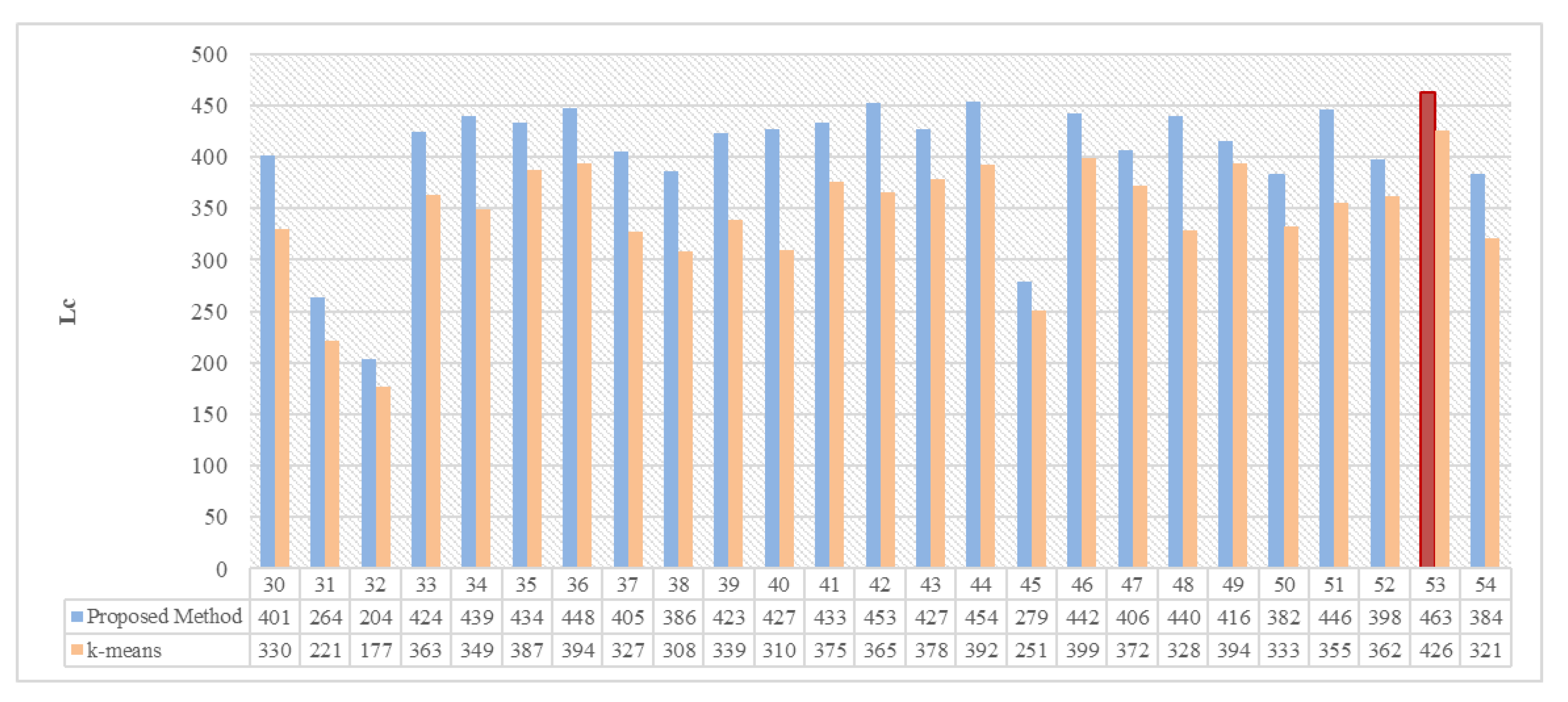
The objective function values L ( c ) (Equation (1b)) corresponding to different numbers c of service units were calculated in this step via enumeration for two clustering methods (the proposed fuzzy clustering method and the classical k-means hard clustering method), and the results are shown in Figure 5. For both the proposed method and the classical method, the L ( c ) values are high for c values of { 36 ,   42 ,   44 ,   51 ,   53 } and reach a peak when c is set to 53 .
Additionally, the performance of k-means is lower than that of the proposed fuzzy clustering method. For example, when c is set to 53 , the L ( c ) value (Equation (1b)) obtained with the proposed clustering method is 8% higher than that obtained with k-means. The difference is even larger (approximately 2%) when c is set to 40. These findings suggest that the proposed soft clustering method is superior to the hard-clustering method.
We selected the number of clusters resulting in the highest L ( c ) , as an example to illustrate the distribution of the service units, as shown in Figure 6. However, this is not necessarily the most appropriate number of service units. After calculating all plans in their entirety, including the service units and service routes, we can evaluate the statistical characteristics of each plan based on the metrics discussed in Section 2.5 to select the optimal number of service units. In our discussion of step (iii), we will further consider the optimal plan for RRD.

3.3.2. Results and Discussion of Step (ii)

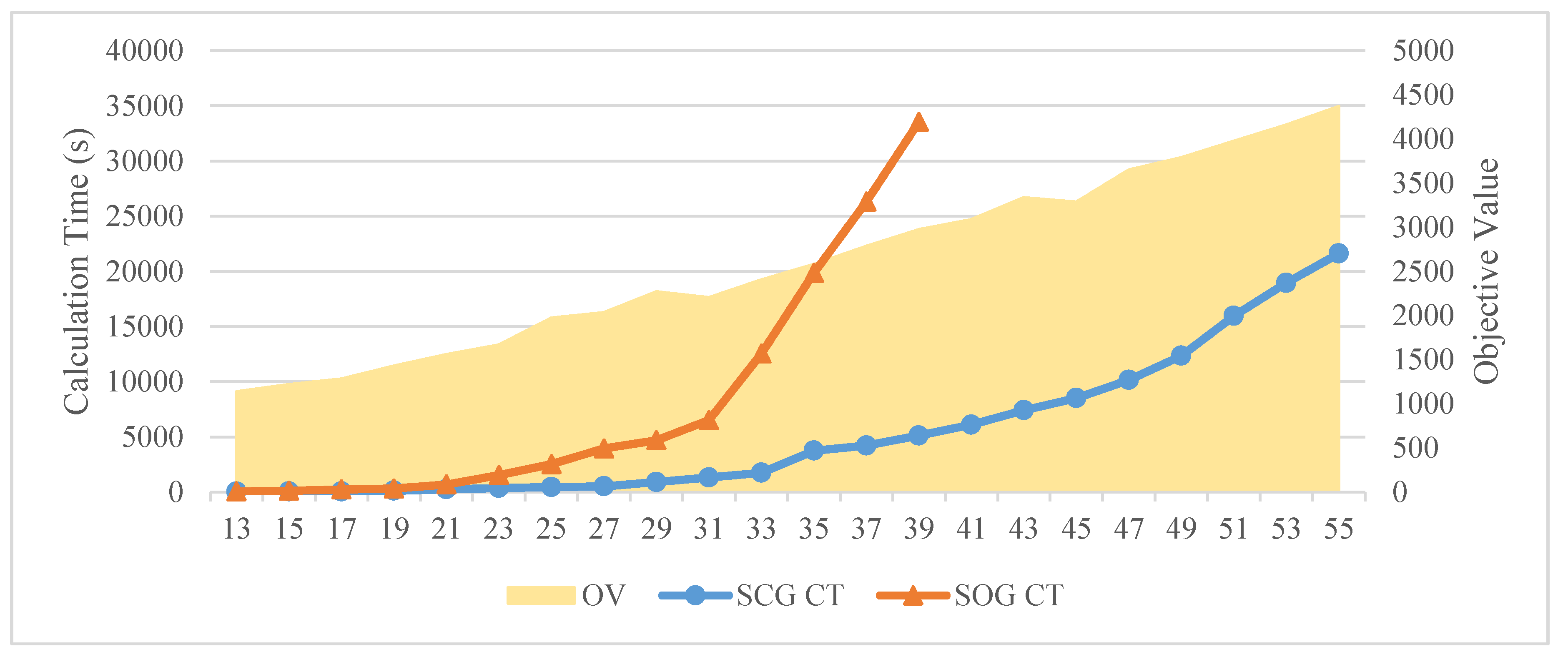
To validate the proposed routing method, problem instances with 13-55 service units were solved to obtain two types of solutions, SOGs and SCGs, where the SOG for a particular problem instance is the solution to R M (discussed in Section 2.1.3) as obtained by GAMS (a commercial solution software), whereas the SCG is the solution to the models M P and S k obtained using the CG algorithm. We regard the SOG as the standard solution to the problem. By comparing the SOGs and SCGs in terms of their objective values and calculation times, we can evaluate whether the proposed method is feasible and efficient.
Figure 7 presents a comparison of the SOGs and SCGs from the perspectives of the calculation times and objective values. The proposed routing method obtains the same results as GAMS does; thus, the proposed method is feasible. Regarding the calculation time, as the number of service units increases, the calculation times for the SCGs exhibit acceptable linear growth when the number of service units is less than 35. As the number of service units increases greater than 35, the calculation time increases significantly. When the number of service units reaches 55, the calculation time is 21,612 s (approximately 6 h), which is essentially the maximum acceptable limit. In contrast, the calculation times for the SOGs indicate that GAMS cannot address large-scale problems (involving approximately 50 service units). With more than 21 service units, the SOG calculation times exhibit much more rapid growth than the SCG calculation times do; when the number of service units is 39, the calculation time for the SOG is 33,541 s (approximately 9.3 h, at least 1.55 times as long as that of our proposed method). These observations demonstrate the effectiveness of the proposed method.
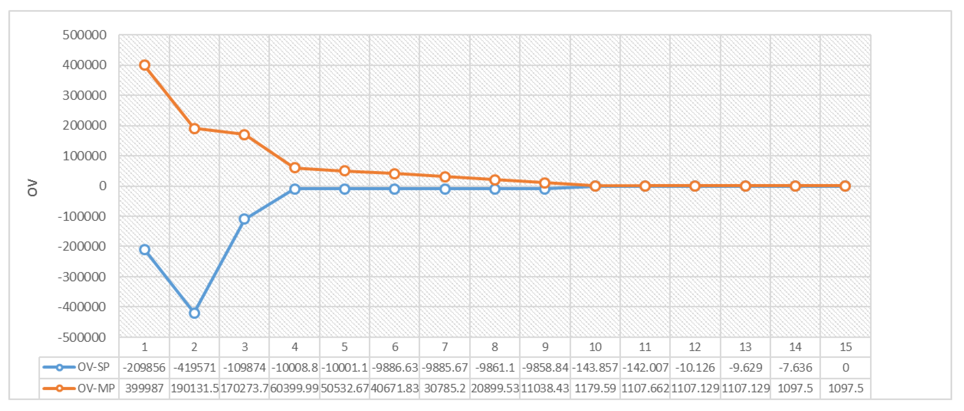
Now, let us consider a case with 13 service units as an example to illustrate how the branching scheme works during the FAR solution process. The edges in this case are indexed by numbers from 0 to 156. The relationship between the objective value and the iteration number throughout the entire solution process is shown in Figure 8. In the 15th iteration, the termination criterion is met. The objective value of the solution is 1097.4995 (with 10 vehicles), and the calculation time is 14,230 ms.
Table 3 presents the details of the original solution obtained with the proposed algorithm. Routes 14, 17, and 22 are fractional; therefore, the solution is not feasible. Consequently, the branching scheme [57] must be applied to guarantee the feasibility of the final solution.
We choose edge 101 as the branching point. After branching, we obtain a left branch and a right branch. The left branch eliminates edges 162, 5, 23, 56, 70, 80, 162, and 193 as well as routes including those edges. By contrast, the right branch forces edge 101 to be selected. From the objective values, we find that the left branch (1139.103) is superior to the right branch (1157.919). The objective value of the left branch is equal to that of the SOG (1139.103).

3.3.3. Results and Discussion of Step (iii)

Based on the various service units generated in step (i), we further planned the routes and evaluated the results using the metrics proposed in Section 2.5 to choose the optimal service plan. The results based on different numbers of service units ( c = { 50 ,   51 ,   52 ,   53 ,   54 } ) are shown in Table 4.
From the perspective of the total passenger cost, as the number of service units increases, the walking time of passengers (and the corresponding generalized cost, c t w ) gradually decreases. This trend is also roughly reflected in the passengers’ travel time (and the corresponding ticket cost, c t t ) and ride time (and the corresponding general cost due to travel time, c g t ), but the following difference is found: when the number of service units is 53, the passengers spend the least time and distance traveling (the corresponding c t t and c g t values are the smallest). The reason for this phenomenon is that these two indicators are jointly determined by the distribution of the service units and the designed routes. In a real-world road network, even a slight change in the service units can result in a change in the routes and, thus, the costs.
From the perspective of the total fleet cost, when the number of service units is in the range of 50-54, the number of rejected requests is not high; in fact, only one request is rejected ( p r = 180 ). When the number of service units is 50-53, the number of vehicles used remains almost constant, being either 19 or 20 ( c f f = 1710   o r   1800 ). When the number of clusters is 54, however, the number of vehicles used increases to 23 ( c f f = 2070 ), which is much greater than the numbers of vehicles used in the other cases. A similar trend is seen in terms of the variable cost ( c v f ), and when the number of service units is 53, the cost is optimal. The reason for this finding may be that the routes corresponding to the specific distribution of the service units in the real-world road network are relatively simple when the number of service units is 53.
In summary, for RRD, the best plan is obtained when the number of service units is 53. In this plan, requesters must walk for approximately 6.8 min ( c t w = 34.00 ) on average, and approximately 13.43 requests are served per service unit.

3.3.4. Results and Discussion of Step (iv)

In this step, we compared the proposed LIPDRS with the existing door-to-door service (based on the model presented in [57]) on various datasets (discussed at the beginning of Section 3). The results are reported in Table 5 and Table 6.
First, building on the results of steps (i) and (iii), we compared the plans designed for the LIPDRS and door-to-door (DtD) options. Regarding the passenger cost, LIPDRS results in a cost of approximately 160,723.46 ( = 17409.55 + 4763.66 + 138550.25 ) CNY, and DtD results in a cost of approximately 269,556.67 ( = 0 + 8959.04 + 260597.63 ) CNY. Obviously, from the passenger’s point of view, LIPDRS costs 40.37% less than DtD. The difference in the general cost due to travel time is the main reason. To meet the LIPP in the real-world road network, the DtD service will require passengers to spend more time on vehicles after boarding, and the corresponding cumulative waiting time will constitute a significant difference in the passengers’ travel expenses. Regarding the fleet cost, LIPDRS costs approximately 4369.43 units, and DtD costs approximately 6804.38 units. Thus, LIPDRS costs approximately 35.79% less than DtD. This difference is due to the establishment of the service units, which greatly reduces the transportation burden placed on the vehicles and thus reduces operating costs. Therefore, in this real-world case, the proposed transport option has an economic advantage.
Next, we analyzed the scope of application of the proposed solution by comparing the two different transport options on the artificial datasets. From ARR to ACR (including ARCR25–75%), the spatiotemporal concentration of requests gradually increases. For LIPDRS, the walking time of passengers (and the corresponding generalized cost, c t w ) is relatively high on ARR. In addition, the c t t and c g t values are high, almost the same as those for the DtD option. In contrast, DtD does not require passengers to walk. Consequently, the total passenger cost (259,834.19 CNY) is lower than that for LIPDRS (314,414.32 CNY). Moreover, LIPDRS also costs more than DtD from the perspective of the fleet cost. These results indicate that LIPDRS lacks adaptability to random and decentralized distributed requests such as those in ARR.
As the level of demand centralization increases (i.e., as the dataset changes from ARR to ARCR25%, ARCR50% and ARCR75%), the c t w value of LIPDRS decreases, and the c t t and c g t values show the same trend. In terms of the fleet cost, LIPDRS begins to cost less than DtD with ARCR50%. At this point, the advantage of LIPDRS begins to emerge. When the ratio of requests that are spatiotemporally concentrated is above 50%, LIPDRS is the more suitable option. Therefore, we believe that the proposed LIPDRS is much more suitable for accommodating the LIPP in a metropolitan context. For example, on ARCR75%, LIPDRS can reduce the cost for passengers by approximately 17.94% and the cost for operators by approximately 32.14%.

4. Conclusions

To alleviate the problems caused by LIPP in metropolises, this paper proposes an innovative type of demand-responsive public transport service called LIPDRS. By providing an attractive transportation option for passengers who typically drive or use conventional public transport, this type of demand-responsive service can potentially reduce car usage and expand passenger accessibility in congested metropolitan areas.
To obtain the optimal operation plan for LIPDRS, we model the LIPDRS decision process using a mixed-integer programming model with dual objectives to optimize the service from the perspectives of both passengers and operators. This model includes a carefully designed passenger walking time constraint and request rejection mechanism to ensure that the resulting service plan can guarantee not only good quality of service but also improved operational efficiency. Additionally, this paper proposes a clustering-first, routing-second framework for solving the proposed model. A modified version of the fuzzy c-means clustering algorithm and a column generation algorithm are utilized in this framework to determine the service units and perform vehicle assignment and routing, respectively. In addition, to overcome the problems caused by relaxing the model variables, a branching scheme is proposed.
Based on the designed methodology, a four-step experiment was conducted to investigate different transport options on various types of datasets. The results demonstrate the advantages of the proposed method and illustrate its application scope. The contributions of this paper can be summarized as follows. (i) We propose a new transport option along with a complete system of modeling and solution methods. A maximum passenger walking time constraint, a request rejection mechanism and a scheme for ensuring solution feasibility are all considered in this scheduling system. (ii) The proposed transport option has been proven to achieve better performance (by 40.37% for passengers and by 35.79% for operators) than the existing “door-to-door” transport option does when faced with LIPP. (iii) By testing on different datasets, we prove that the proposed service is more suitable for the request distributions that are spatiotemporally concentrated. We have found that when the ratio of requests that are spatiotemporally concentrated is above 50%, LIPDRS is the more suitable option. (iv) The performance advantages of the proposed clustering-first, routing-second solving framework have been proven through experiments. Regarding the individual components of the framework, the proposed soft clustering algorithm has been proven to be superior to the k-means hard clustering method (by 8%), and the proposed routing algorithm has been proven to be 1.5 times more efficient than the commercial solution software GAMS.
Overall, the proposed methodology has the following attractive features for solving the issues faced due to LIPP in metropolitan contexts: (i) The service considers the trade-off between operator profit and requester cost. (ii) At the expense of increasing the passengers’ walking times, the proposed service can effectively reduce the passengers’ ride times and the operating costs of the fleet relative to existing door-to-door services. This service is suitable for use in cases of insufficient capacity. The LIPDRS approach can also be used for the scheduling of liquefied natural gas (LNG) buses or pure electric buses. Additionally, it can be used for transport between residential areas and central business districts and for acyclic transportation related to holidays and large events. The use of this mode of transport can help to support green and sustainable metropolitan development.
In this study, only one type of vehicle is considered for LIPDRS planning. However, for a metropolis with diverse demands, this assumption is not appropriate. In future research, we will consider hybrid fleets with different types of vehicles (e.g., with different speeds and capacities) to improve both operator profits and passenger costs. In addition, the whole LIPDRS design process requires some preliminary preparation time for finding the optimal c value, which limits the capability of online implementation. Therefore, we will seek improvements in computational efficiency in future research. For example, some intelligent optimization methods [61,62,63] or cloud computing techniques [64] can be used to obtain solutions efficiently.

Author Contributions

Conceptualization, H.Z.; Methodology, H.Z.; Project administration, X.Z.; Resources, X.Z.; Software, H.Z.; Supervision, J.C.; Visualization, Z.Y.; Writing—original draft, H.Z.

Funding

The research is supported by the National Key R&D Program of China (Grant No. 2018YFB1201401) and the National Natural Science Foundation of China (Grant No. U1734204).

Conflicts of Interest

The authors declare no conflict of interest.

References

  1. Liu, T.; Ceder, A.; Bologna, R.; Cabantous, B. Commuting by customized bus: A comparative analysis with private car and conventional public transport in two cities. J. Public Transp. 2016, 19, 55–74. [Google Scholar] [CrossRef]
  2. Zhao, P.; Hu, H. Geographical patterns of traffic congestion in growing megacities: Big data analytics from beijing. Cities 2019, 92, 164–174. [Google Scholar] [CrossRef]
  3. Wu, W.; Wang, M.X.; Zhang, F. Commuting behavior and congestion satisfaction: Evidence from Beijing, China. Transp. Res. Part D Transp. Environ. 2019, 67, 553–564. [Google Scholar] [CrossRef]
  4. Saneinejad, S.; Roorda, M.J.; Kennedy, C. Modelling the impact of weather conditions on active transportation travel behaviour. Transp. Res. Part D 2012, 17, 129–137. [Google Scholar] [CrossRef] [Green Version]
  5. Lu, T.; Zhou, L.; Liu, J.; Zhou, X. Customized bus service design for jointly optimizing passenger-to-vehicle assignment and vehicle routing. Transp. Res. Part C Emerg. Technol. 2017, 85, 451–475. [Google Scholar]
  6. Dumas, Y.; Desrosiers, J.; Soumis, F. Large Scale Multi-Vehicle Dial-a-Ride Problems; École des Hautes Études Commerciales: Paris, France, 1989. [Google Scholar]
  7. Zhang, K.; Sun, D.; Shen, S.; Zhu, Y. Analyzing spatiotemporal congestion pattern on urban roads based on taxi gps data. J. Transp. Land Use 2017, 10, 675–694. [Google Scholar] [CrossRef]
  8. Martínez, L.M.; Viegas, J.M.; Eiró, T. Formulating a new express minibus service design problem as a clustering problem. Transp. Sci. 2014, 49, 85–98. [Google Scholar] [CrossRef]
  9. Park, J.; Kim, B.I. The school bus routing problem: A review. Eur. J. Oper. Res. 2010, 202, 311–319. [Google Scholar] [CrossRef]
  10. Cain, A.; Darido, G.; Baltes, M.; Rodriguez, P.; Barrios, J. Applicability of transmilenio bus rapid transit system of bogotá, colombia, to the united states. Transp. Res. Record. 2007, 2034. [Google Scholar] [CrossRef]
  11. Pan, G.; Qi, G.; Zhang, D.; Zhang, D.; Li, S. Land-use classification using taxi gps traces. IEEE Trans. Intell. Transp. Syst. 2013, 14, 113–123. [Google Scholar] [CrossRef]
  12. Idris, H.; Clarke, J.P.; Bhuva, R.; Kang, L. Queuing model for taxi-out time estimation. Air Traffic Control Q. 2001, 10, 1–22. [Google Scholar] [CrossRef]
  13. Lee, D.H.; Wang, H.; Cheu, R.L.; Teo, S.H. A taxi dispatch system based on current demands and real-time traffic conditions. Transp. Res. Rec. J. Transp. Res. Board 2004, 1882. [Google Scholar] [CrossRef]
  14. Ritzinger, U.; Puchinger, J.; Hartl, R.F. Dynamic programming based metaheuristics for the dial-a-ride problem. Ann. Oper. Res. 2016, 236, 341–358. [Google Scholar] [CrossRef]
  15. Parragh, S.N.; Jorge, P.D.S.; Almada-Lobo, B. The dial-a-ride problem with split requests and profits. Transp. Sci. 2014, 49, 311–334. [Google Scholar] [CrossRef]
  16. Clarens, G.C.; Hurdle, V.F. An operating strategy for a commuter bus system. Transp. Sci. 1975, 9, 1–20. [Google Scholar] [CrossRef]
  17. Larrain, H.; Muñoz, J.C. When and where are limited-stop bus services justified? Transp. A Transp. Sci. 2016, 12, 811–831. [Google Scholar] [CrossRef]
  18. Ren, Y.; Chen, G.; Han, Y.; Zheng, H. Extracting Potential Bus Lines of Customized City Bus Service Based on Public Transport Big Data; IOP Publishing: Bristol, UK, 2016; Volume 46, p. 012017. [Google Scholar]
  19. Ma, J.; Yang, Y.; Guan, W.; Wang, F.; Liu, T.; Tu, W.; Song, C. Large-scale demand driven design of a customized bus network: A methodological framework and beijing case study. J. Adv. Transp. 2017, 2017. [Google Scholar] [CrossRef]
  20. Walteros, J.L.; Medaglia, A.L.; Riaño, G. Hybrid algorithm for route design on bus rapid transit systems. Transp. Sci. 2015, 49, 66–84. [Google Scholar] [CrossRef]
  21. Ma, J.; Zhao, Y.; Yang, Y.; Liu, T.; Wei, G.; Wang, J.; Song, C. A model for the stop planning and timetables of customized buses. PLoS ONE 2017, 12, e0168762. [Google Scholar] [CrossRef]
  22. Sun, D.J.; Xu, Y.; Peng, Z.R. Timetable optimization for single bus line based on hybrid vehicle size model. J. Traffic Transp. Eng. 2015, 2, 179–186. [Google Scholar] [Green Version]
  23. Schittekat, P.; Kinable, J.; Sörensen, K.; Sevaux, M.; Spieksma, F.; Springael, J. A metaheuristic for the school bus routing problem with bus stop selection. Eur. J. Oper. Res. 2013, 229, 518–528. [Google Scholar] [CrossRef]
  24. Shaheen, S.A. Commuter-based carsharing: Market niche potential. Transp. Res. Rec. J. Transp. Res. Board 2001, 1760, 178–183. [Google Scholar] [CrossRef]
  25. Katzev, R. Car sharing: A new approach to urban transportation problems. Anal. Soc. Issues Public Policy 2003, 3, 65–86. [Google Scholar] [CrossRef]
  26. Kek, A.G.H.; Cheu, R.L.; Meng, Q.; Fung, C.H. A decision support system for vehicle relocation operations in carsharing systems. Transp. Res. Part E 2009, 45, 149–158. [Google Scholar] [CrossRef]
  27. Shaheen, S.A.; Cohen, A.P. Carsharing and personal vehicle services: Worldwide market developments and emerging trends. Int. J. Sustain. Transp. 2013, 7, 5–34. [Google Scholar] [CrossRef]
  28. Cullen, F.H.; Jarvis, J.J.; Ratliff, H.D. Set partitioning based heuristics for interactive routing. Networks 1981, 11, 125–143. [Google Scholar] [CrossRef]
  29. Bodin, L.D.; Sexton, T. The multi-vehicle subscriber dial-a-ride problem. Tims Stud. Manag. Sci. 1986, 26, 73–86. [Google Scholar]
  30. Sexton, T.R.; Bodin, L.D. Optimizing single vehicle many-to-many operations with desired delivery times: I. Scheduling. Transp. Sci. 1985, 19, 378–410. [Google Scholar] [CrossRef]
  31. Sexton, T.R.; Bodin, L.D. Optimizing single vehicle many-to-many operations with desired delivery times: II. Routing. Transp. Sci. 1985, 19, 411–435. [Google Scholar] [CrossRef]
  32. Desrosiers, J.; Dumas, Y.; Soumis, F.; Taillefer, S.; Villeneuve, D. An Algorithm for Mini-Clustering in Handicapped Transport. Cah. Du Gerad. 1991. Available online: https://www.researchgate.net/publication/245275603_An_algorithm_for_mini-clustering_in_handicapped_transport (accessed on 12 September 2019).
  33. Ioachim, I.; Desrosiers, J.; Dumas, Y.; Solomon, M.M.; Villeneuve, D. A request clustering algorithm for door-to-door handicapped transportation. Transp. Sci. 1995, 29, 63–78. [Google Scholar] [CrossRef]
  34. Pankratz, G. A grouping genetic algorithm for the pickup and delivery problem with time windows. Or. Spectr. 2005, 27, 21–41. [Google Scholar] [CrossRef]
  35. Bard, J.F.; Jarrah, A.I. Large-scale constrained clustering for rationalizing pickup and delivery operations. Transp. Res. Part B Methodol. 2009, 43, 542–561. [Google Scholar] [CrossRef]
  36. Qu, Y.; Bard, J.F. A grasp with adaptive large neighborhood search for pickup and delivery problems with transshipment. Comput. Oper. Res. 2012, 39, 2439–2456. [Google Scholar] [CrossRef]
  37. Masson, R.; Lehuédé, F.; Péton, O. An adaptive large neighborhood search for the pickup and delivery problem with transfers. Transp. Sci. 2013, 47, 344–355. [Google Scholar] [CrossRef]
  38. Toth, P.; Vigo, D. An Overview of Vehicle Routing Problems; Society for Industrial and Applied Mathematics: Philadelphia, PA, USA, 2001; pp. 1–26. [Google Scholar]
  39. Toth, P.; Vigo, D. The Vehicle Routing Problem; Tsinghua University Press: Beijing, China, 2011; pp. 127–153. [Google Scholar]
  40. Parragh, S.N.; Doerner, K.F.; Hartl, R.F. A survey on pickup and delivery problems. Manag. Rev. Q. 2008, 58, 21–51. [Google Scholar]
  41. Paquette, J.; Cordeau, J.F.; Laporte, G.; Pascoal, M.M.B. Combining multicriteria analysis and tabu search for dial-a-ride problems. Transp. Res. Part B Methodol. 2013, 52, 1–16. [Google Scholar] [CrossRef] [Green Version]
  42. Cordeau, J.F.; Laporte, G.; Potvin, J.Y.; Savelsbergh, M.W.P. Transportation on demand. Handb. Oper. Res. Manag. Sci. 2007, 14, 429–466. [Google Scholar]
  43. Fisher, M.L.; Jaikumar, R. A generalized assignment heuristic for vehicle routing. Networks 1981, 11, 109–124. [Google Scholar] [CrossRef]
  44. Fisher, M.L.; Jörnsten, K.O. Vehicle routing with time windows: Two optimization algorithms. Oper. Res. 1997, 45, 488–492. [Google Scholar] [CrossRef]
  45. Sol, M. Column Generation Techniques for Pickup and Delivery Problems; Technische Universiteit Eindhoven: Eindhoven, The Netherlands, 1994. [Google Scholar]
  46. Parragh, S.N.; Schmid, V. Hybrid column generation and large neighborhood search for the dial-a-ride problem. Comput. Oper. Res. 2013, 40, 490–497. [Google Scholar] [CrossRef] [Green Version]
  47. Ropke, S.; Cordeau, J.F.; Laporte, G. Models and Branch-and-Cut Algorithms for Pickup and Delivery Problems With Time Windows; Wiley-Interscience: Hoboken, NJ, USA, 2007; pp. 258–272. [Google Scholar]
  48. Masson, R.; Ropke, S.; Lehuédé, F.; Péton, O. A branch-and-cut-and-price approach for the pickup and delivery problem with shuttle routes. Eur. J. Oper. Res. 2014, 236, 849–862. [Google Scholar] [CrossRef]
  49. Cordeau, J.F.; Laporte, G. A tabu search heuristic for the static multi-vehicle dial-a-ride problem. Transp. Res. Part B Methodol. 2003, 37, 579–594. [Google Scholar] [CrossRef] [Green Version]
  50. Stiglic, M.; Agatz, N.; Savelsbergh, M.; Gradisar, M. The benefits of meeting points in ride-sharing systems. Transp. Res. Part B 2015, 82, 36–53. [Google Scholar] [CrossRef] [Green Version]
  51. Li, Y.; Yu, F. A new validity function for fuzzy clustering. In Proceedings of the International Conference on Computational Intelligence and Natural Computing, Wuhan, China, 6–9 June 2009; pp. 462–465. [Google Scholar]
  52. Fahad, A.; Alshatri, N.; Tari, Z.; Alamri, A.; Khalil, I.; Zomaya, A.Y.; Foufou, S.; Bouras, A. A survey of clustering algorithms for big data: Taxonomy and empirical analysis. Emerg. Top. Comput. IEEE Trans. 2014, 2, 267–279. [Google Scholar] [CrossRef]
  53. Savas, E.S. On equity in providing public services. Manag. Sci. 1978, 24, 800–808. [Google Scholar] [CrossRef]
  54. Bezdek, J.C.; Ehrlich, R.; Full, W. Fcm: The fuzzy c-means clustering algorithm. Comput. Geosci. 1984, 10, 191–203. [Google Scholar] [CrossRef]
  55. Luxburg, U.V. A tutorial on spectral clustering. Stat. Comput. 2007, 17, 395–416. [Google Scholar] [CrossRef]
  56. Bezdek, J.C. A convergence theorem for the fuzzy isodata clustering algorithms. IEEE Trans. Pattern Anal. Mach. Intell. 1980, 2, 1–8. [Google Scholar] [CrossRef]
  57. Feillet, D. A tutorial on column generation and branch-and-price for vehicle routing problems. 4OR 2010, 8, 407–424. [Google Scholar] [CrossRef]
  58. Dumas, Y.; Desrosiers, J.; Soumis, F. The pickup and delivery problem with time windows. Eur. J. Oper. Res. 1991, 54, 7–22. [Google Scholar] [CrossRef]
  59. O’Sullivan, S.; Morrall, J. Walking distances to and from light-rail transit stations. Transp. Res. Rec. J. Transp. Res. Board 1996, 1538, 19–26. [Google Scholar] [CrossRef]
  60. Kumar, C.V.P.; Basu, D.; Maitra, B. Modeling generalized cost of travel for rural bus users: A case study. J. Public Transp. 2004, 7, 4. [Google Scholar] [CrossRef]
  61. Gao, K.; Cao, Z.; Zhang, L.; Chen, Z.; Han, Y.; Pan, Q.J. A review on swarm intelligence and evolutionary algorithms for solving flexible job shop scheduling problems. IEEE/CAA J. Autom. Sinica 2019, 6, 904–916. [Google Scholar] [CrossRef]
  62. Zhao, J.; Liu, S.; Zhou, M.; Guo, X.; Qi, L. Modified cuckoo search algorithm to solve economic power dispatch optimization problems. IEEE/CAA J. Autom. Sinica 2018, 5, 794–806. [Google Scholar] [CrossRef]
  63. Bi, J.; Yuan, H.; Tan, W.; Zhou, M.; Fan, Y.; Zhang, J.; Li, J. Application-aware dynamic fine-grained resource provisioning in a virtualized cloud data center. IEEE Trans. Autom. Sci. Eng. 2015, 14, 1172–1184. [Google Scholar] [CrossRef]
  64. Li, W.; Xia, Y.; Zhou, M.; Sun, X.; Zhu, Q. Fluctuation-aware and predictive workflow scheduling in cost-effective infrastructure-as-a-service clouds. IEEE Access 2018, 6, 61488–61502. [Google Scholar] [CrossRef]
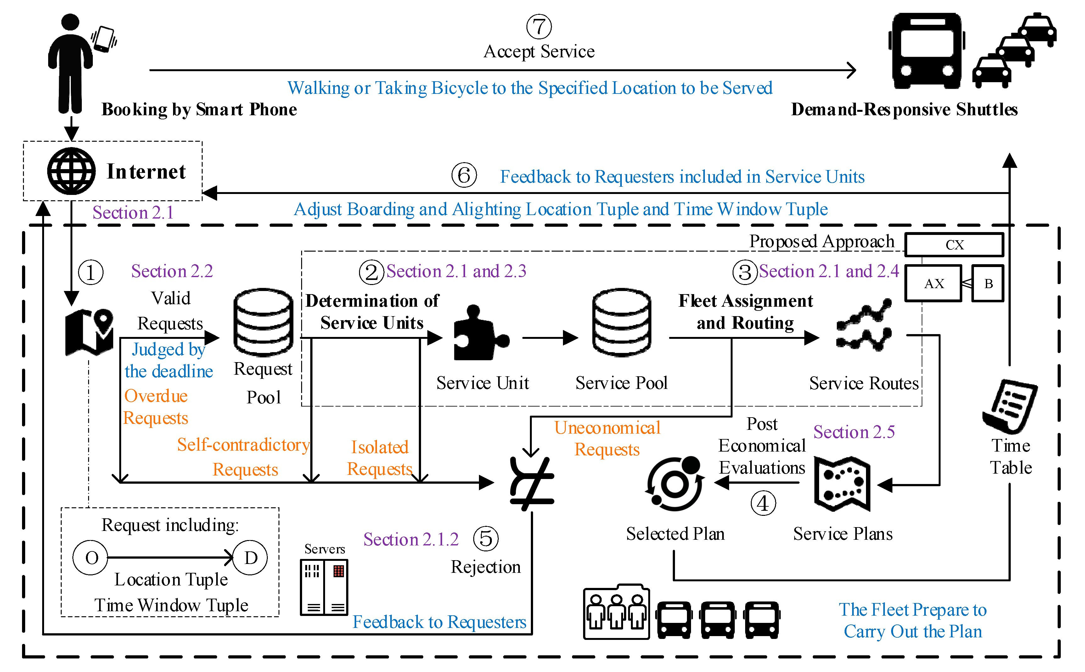
Figure 1. The Planning Process of a Demand-Responsive Express Shuttle Service. In this figure, the critical steps are labeled by numbers that are corresponding to the content of Section 2.1.1. Additionally, the subsections (that present detailed expressions about elements in this figure) are labeled to help understand the entire methodology structure.
Sustainability 11 05025 g001
Figure 2. Illustration of the LIPDRS design model (LIPPD). This figure demonstrates the main optimization content of the proposed model, from the bottom to the top. There are three types of nodes in this figure, where the cycles represent requests (the diagonal striped circles represent origins, and the striped circles represent destination); the squares represent boarding parts and alighting parts of service units (the diagonal striped squares represent selected boarding parts, the striped squares represent selected alighting parts, the filled squares represent the candidate boarding parts, and the blank squares represent the candidate alighting parts). Both the boarding part and the alighting part include information about location and time window. The figure shows the process of design service units and service routes from requests that exists in the optimization model. In the middle and the bottom of the figure, requests are assigned to service units according to spatiotemporal features of the requests and constraints. Then, in the top of the figure, the boarding parts and alighting parts of service units are assigned to service routes and to be served by the vehicles in the fleet.
Sustainability 11 05025 g002
Figure 3. Determination of service units (DSU) flows.
Sustainability 11 05025 g003
Figure 4. FAR Flows.
Sustainability 11 05025 g004
Figure 5. Values of L ( c ) with various c values. This figure shows the comparison of the proposed method with the classical k-means. It can be clearly observed from the figure that the L ( c ) values of the two methods have similar trends, but the proposed method has obvious advantages. This advantage is related to the application of the Gaussian kernel function. In addition, the figure expresses the changes in the index L ( c ) with the value of c . When c is less than 34, the L ( c ) value tends to decrease monotonically. When c is greater than 34, the L value fluctuates and reaches a maximum at c = 53 .
Sustainability 11 05025 g005
Figure 6. Distribution of 53 service units. This figure illustrates the distribution of requests and service units. To present a readable illustration of the distribution, the cluster centers are drawn on the left, and the requests are drawn on the middle, on the same space range. The legend of clusters is shown on the right. From this figure, it can be observed that the service units obtained by the algorithm are reasonable. This observation can help us set the proper service units.
Sustainability 11 05025 g006
Figure 7. Comparison of SOGs and SCGs: OV represents the objective value, and CT represents the calculation time.
Sustainability 11 05025 g007
Figure 8. Convergence curve of the proposed CG-based algorithm.
Sustainability 11 05025 g008
Table 1. Comparison of various urban public transport options.
Name 1Schedule
Frequency
TD 2Decision
Basis
Request
Method
Service
Locations
P 3C 4R 5
TaxiN/AOIDN/AEncountersUncertainHH[11,12,13]
DARSFlexibleOIDOD information, preferred arrival/departure timesPhone/Internet bookingsOD pointsHH[14,15]
TCSFixed frequencyRMDHistorical informationSurveys/consultationBus stationsLL[16,17]
CB Flexible frequencyRMDEstimated OD informationSurveys/historical dataBus stationsLM[1,18,19,20,21,22]
SBFixed routesRMDRegistered informationSchool recordsHome and schoolLH[9,23]
CSFlexibleOIDOD information, preferred arrival/departure timesPhone/Internet bookingsFixed
B&A6
LM[24,25,26,27]
LIPDRSDetermined based on dynamic requestsOMDAggregated OD information and preferred arrival/departure timesPhone/Internet bookingsDynamic
B&A6
LMThis study
1 DARS: Dial-a-ride service; TCS: Traditional conventional shuttle; CB: Customized bus; SBRP: School bus; CS: Car-sharing service; LIPDRS: Large-scale instantaneous-peak-demand-responsive express shuttle service. 2 TD: Target demands; OID: Occasional individual demands; RMD: Regular massive demands; OMD: Occasional massive demands. 3 P: Price; H: High; L: Low. 4 C: Convenience: H: High; M: Moderate; L: Low. 5 R: Reference. 6 B&A: Boarding and alighting locations.
Table 2. Parameter settings.
IDParameter NameValueUnitSource
1Maximum walking time, m w t 5min[59]
2Set of candidate numbers of service units, c c { 30 ,   31 , , 53 ,   54 } Estimated
3Operation time redundancy, ς 15minSurvey
4Threshold, ε 0.001 [54]
5Maximum number of iterations, m i 200 [7]
6Unit cost of a vehicle, C V 1 4unit/km[57]
7Fixed cost of a vehicle, C F 90 4units[57]
8Penalty value for canceling a request, p r 180 4unitsSurvey
9Cost that passengers expect to incur for additional walking time (CNY/min), C P W 5CNY/minSurvey
10Maximum operating distance, d m a x 240kmSurvey
11Maximum driving time, t m a x 360minSurvey
12Vehicle capacity, Q 56 Survey
13Fleet size, | M | 50 Setting
14Vehicle operating speedESRN 3km/hDigital map
15Fixed price for using the service, P F 1CNYSurvey 1
16Variable price for using the service, P V 0.25CNY/kmSurvey 1
17Generalized cost of using the service, C G 400CNY/h[60]
18Depot location 2Lat: 40.0521, Lng: 116.3085 Survey
1 According to the carpooling price for Didi in Beijing. 2 We used a currently operating bus hub as the depot. 3 Expected speed in the road network (ESRN), obtained from ‘AMAP’, a digital map. 4 In the context of our study, we regard the travel distance as being proportional to the travel cost. However, the proportionality between travel distance and cost is not a key element of our study. Therefore, we use a conceptual unit to bypass the proportion determination problem, following reference [57]. According to survey data, the average fuel consumption of a large bus is approximately 0.3–0.35 L/km. Based on the price of diesel in Beijing, one unit corresponds to approximately 2 CNY.
Table 3. Original solution obtained with the proposed CG-based algorithm (Routes and Edges).
Route ID14151718192021222325
Value0.510.511110.511
Edge ID21011441115098671085614271
Value0.50.50.50.50.50.50.50.50.50.50.5
Calculation time14,230 ms
Objective value1097.4995
Iterations15
Table 4. Statistical analysis of plans with c = { 50 ,   51 ,   52 ,   53 ,   54 }
c Total Passenger Cost (CNY)Total Fleet Cost (Units)
c t w   1 c t t   2 c g t   3 c f f   4 c v f   5 p r   6
5030263.68 7152.60 208046.58 1710.00 2405.50 180.00
5128127.17 6917.87 201217.97 1800.00 2453.49 180.00
5226703.37 6932.35 201639.24 1800.00 2498.54 180.00
5324211.44 6624.00 192669.20 1800.00 2389.43 180.00
5423498.54 6829.69 198652.70 2070.00 2502.57 180.00
c Average and Standard Deviation of Passenger Cost (CNY)Average and Standard Deviation of Fleet Cost (units)
c t w c t t c g t c f f c v f p r
5042.51±6.15 10.05±2.78 292.20±14.89 90.00±0 126.61±21.37 180.00±0
5139.50±4.69 9.72±3.74 282.61±12.64 90.00±0 122.67±20.14 180.00±0
5237.51±4.05 9.74±4.29 283.21±9.96 90.00±0 124.93±18.48 180.00±0
5334.00±5.59 9.30±2.88 270.60±12.31 90.00±0 119.47±15.12 180.00±0
5433.00±5.08 9.59±3.21 279.01±14.87 90.00±0108.81±14.15 180.00±0
1 c t w Walking cost, c t w = C P W · T T W , where C P W represents the cost that passengers expect to incur for additional walking time (CNY/min) and T T W represents the total walking time (min). 2 c t t : Ticket cost, c t t = P F · N S + P V · D T P V , where P V is the unit variable price for using the service, P F is the fixed price for using the service, N S is the number of requests served, and D T P V represents the total distance traveled by all passengers in vehicles (km). 3 c g t : General cost due to travel time, c g t = C G · T T P V , where C G represents the unified generalized cost (in terms of time and comfort) of passengers using the service and T T P V represents the total time spent by all passengers in vehicles. 4 c f f : Fixed cost of the fleet, c f f = N · C F , where N is the number of vehicles used and C F is the unit fixed cost of using a vehicle. 5 c v f : Variable cost of the fleet, c v f = C V · D T T V , where C V is the unit variable cost of using a vehicle and D T T V represents the total distance traveled by vehicles (km). 6 p r : Rejection penalty, p r = N R R · P R R , where N R R is the number of rejected requests and P R R is the penalty cost for rejecting a request.
Table 5. Comparison of different transport options on various datasets (Total Value).
DatasetTransport OptionTotal Passenger Cost (CNY)Total Fleet Cost (Units)
c t w   1 c t t   2 c g t   3 c f f   4 c v f   5 p r   6
RRDLIPDRS17409.55 4763.66 138550.25 1800.00 2389.43 180.00
DtD0.00 8959.04 260597.63 2790.00 4014.38 0.00
ARRLIPDRS58562.81 8503.62 247348.89 2520.00 3657.60 3960.00
DtD0.00 8635.94 251198.25 2700.00 4069.15 0.00
ARCR
25%
LIPDRS44964.53 8327.44 242223.61 2340.00 3212.11 1800.00
DtD0.00 8900.32 258889.43 2610.00 3956.89 0.00
ARCR
50%
LIPDRS31222.60 7005.99 203781.57 2160.00 3015.32 1440.00
DtD0.00 7901.70 229838.41 2700.00 3957.64 0.00
ARCR
75%
LIPDRS23392.24 6682.68 194376.27 1890.00 2489.66 360.00
DtD0.00 9091.06 264438.16 2970.00 4014.27 0.00
ACRLIPDRS13457.35 6418.37 186687.16 1620.00 2401.47 180.00
DtD0.00 9282.13 269996.44 2610.00 3981.22 0.00
1 c t w : Walking cost, c t w = C P W · T T W , where C P W represents the cost that passengers expect to incur for additional walking time (CNY/min) and T T W represents the total walking time (min). 2 c t t : Ticket cost, c t t = P F · N S + P V · D T P V , where P V is the unit variable price for using the service, P F is the fixed price for using the service, N S is the number of requests served, and D T P V represents the total distance traveled by all passengers in vehicles (km). 3 c g t : General cost due to travel time, c g t = C G · T T P V , where C G represents the unified generalized cost (in terms of time and comfort) of passengers using the service and T T P V represents the total time spent by all passengers in vehicles. 4 c f f : Fixed cost of the fleet, c f f = N · C F , where N is the number of vehicles used and C F is the unit fixed cost of using a vehicle. 5 c v f : Variable cost of the fleet, c v f = C V · D T T V , where C V is the unit variable cost of using a vehicle and D T T V represents the total distance traveled by vehicles (km). 6 p r : Rejection penalty, p r = N R R · P R R , where N R R is the number of rejected requests and P R R is the penalty cost for rejecting a request.
Table 6. Comparison of different transport options on various datasets (Average and Standard Deviation Value).
DatasetTransport OptionAverage and Standard Deviation of Passenger Cost (CNY)Average and Standard Deviation of Fleet Cost (units)
c t w   1 c t t   2 c g t   3 c f f   4 c v f   5 p r   6
RRDLIPDRS34.00 ± 5.59 9.30 ± 3.88 270.60 ± 12.31 90.00 ± 0 119.47 ± 15.12 180.00 ± 0
DtD0.00 12.58 ± 3.25 366.01 ± 11.69 90.00 ± 0129.50 ± 16.27 0.00
ARRLIPDRS82.25 ± 15.1411.94 ± 2.69 347.40 ± 18.74 90.00 ± 0130.63 ± 12.48 180.00 ± 0
DtD0.00 12.13 ± 2.28 352.81 ± 21.67 90.00 ± 0135.64 ± 14.27 0.00
ARCR
25%
LIPDRS63.15 ± 10.48 11.70 ± 2.99 340.20 ± 18.12 90.00 ± 0123.54 ± 13.64 180.00 ± 0
DtD0.00 12.50 ± 3.47 363.61 ± 18.97 90.00 ± 0136.44 ± 13.78 0.00
ARCR
50%
LIPDRS43.85 ± 8.79 9.84 ± 3.47 286.21 ± 15.36 90.00 ± 0125.64 ± 14.27 180.00 ± 0
DtD0.00 11.10 ± 2.49 322.81 ± 21.48 90.00 ± 0131.92 ± 14.68 0.00
ARCR
75%
LIPDRS32.85 ± 6.01 9.39 ± 2.18 273.00 ± 12.21 90.00 ± 0118.56 ± 14.96 180.00 ± 0
DtD0.00 12.77 ± 1.98 371.40 ± 13.74 90.00 ± 0121.64 ± 17.01 0.00
ACRLIPDRS18.90 ± 5.57 9.01 ± 2.01 262.20 ± 14.27 90.00 ± 0133.42 ± 14.12 180.00 ± 0
DtD0.00 13.04 ± 2.57 379.21 ± 20.13 90.00 ± 0137.28 ± 15.21 0.00
1 c t w : Walking cost, c t w = C P W · T T W , where C P W represents the cost that passengers expect to incur for additional walking time (CNY/min) and T T W represents the total walking time (min). 2 c t t : Ticket cost, c t t = P F · N S + P V · D T P V , where P V is the unit variable price for using the service, P F is the fixed price for using the service, N S is the number of requests served, and D T P V represents the total distance traveled by all passengers in vehicles (km). 3 c g t : General cost due to travel time, c g t = C G · T T P V , where C G represents the unified generalized cost (in terms of time and comfort) of passengers using the service and T T P V represents the total time spent by all passengers in vehicles. 4 c f f : Fixed cost of the fleet, c f f = N · C F , where N is the number of vehicles used and C F is the unit fixed cost of using a vehicle. 5 c v f : Variable cost of the fleet, c v f = C V · D T T V , where C V is the unit variable cost of using a vehicle and D T T V represents the total distance traveled by vehicles (km). 6 p r : Rejection penalty, p r = N R R · P R R , where N R R is the number of rejected requests and P R R is the penalty cost for rejecting a request.