Risk Assessment for Engagement in Sharing Economy of Manufacturing Enterprises: A Matter–Element Extension Based Approach

Abstract

At present, manufacturing enterprises in China and across the world are undergoing a critical period of transformation and upgrading for sustainable development, with various obstacles such as financing difficulties and imperfect production facilities. The emergence of the sharing economy may provide a feasible solution for manufacturing enterprises, but meanwhile, unpredictable risks are bound to arise in the process of Engagement in the Sharing Economy of Manufacturing Enterprises (ESEME), and the assessment for the risk of ESEME is an important issue that requires special attention. Based on the characteristics of ESEME, a risk assessment indicator system is constructed, and a matter–element extension based approach is proposed to assess the risk of ESEME. The comprehensive risk value of ESEME can be calculated, and by means of sensitivity analysis and combinatory analysis, sensitive risk indicators and the risk type of indicators are identified. The innovation is embodied in three aspects: the sharing economy is studied by the matter–element extension method, the minimum deviation weight is adopted, and the risk is identified by sensitivity analysis and combinatory analysis. This assessment method is applied to enterprise E, and good results are obtained. This work is conducive to promoting manufacturing enterprises to engage in the sharing economy, which provides an effective vision for enterprises to implement risk management strategies, and also offers references for the government to formulate relevant policies for ESEME.

1. Introduction

The manufacturing industry plays an important role in promoting the world economy [1]. With the rapid development of information technology, the Internet is promoting the transformation of industrial structures, and modern manufacturing enterprises are undergoing a critical period of transformation, upgrading and leapfrogging development [2]. In recent years, great changes have taken place in the social environment faced by the manufacturing industry, such as increasingly fierce global market competition and diversified customer demands [3]. Due to the transformation of the economic situation in China, the gradual rise of labor costs, the weakening of the demographic dividend advantage, and the tightening of environmental and resource constraints, manufacturing enterprises that want to develop better face enormous challenges [4,5]. As a major component of the manufacturing industry, small and medium-sized manufacturing enterprises are also playing an increasingly important role in promoting national economic growth, increasing employment opportunities, promoting technological innovation, and maintaining social stability. However, the management and operation of enterprises have become more and more complex, which reduces the adaptability of organizational capability and technology research and development capability [6]. In the process of production and operation, small and medium-sized manufacturing enterprises often encounter some tough problems, such as a lack of funds, incomplete production facilities, and immature production technology [7]. These issues have limited the sustainable development of small and medium-sized manufacturing enterprises, which has been severely squeezed in the increasingly fierce market competition. What small and medium-sized manufacturing enterprises should focus on is how to manage and improve existing key factors and achieve sustainable growth, and these key factors include productivity, quality, and flexibility [8].

The sharing economy, which is also known as “collaborative consumption” or the “collaborative economy”, was first proposed by professor Marcus Felson and professor Joel Spaeth in 1978, and defined those events in which one or more persons consume economic goods or services in the process of engaging in joint activities with one or more others [9]. Over time, the significance of the sharing economy is also changing. We agree that the operation of the sharing economy depends on the Internet platform, on which people can allocate underutilized resources and get compensation, or get resources and pay corresponding fees [10,11]. In recent years, due to the rapid development of mobile Internet and information technology, the sharing economy, a new business model, has attracted much attention and achieved success on a global scale [12]. The sharing platform, an important component of the sharing economy business model rather than the traditional business model, relies on the Internet to act as an intermediary between suppliers and demanders [13]. Contrary to the traditional business model based on ownership, the sharing economy is established on the use and sharing of products and services, which emphasizes the right to use resources rather than the transfer of ownership [14,15]. The sharing economy is different from the traditional business model and even surpasses it, which disaggregates resources and services in time and space; thereby, it has become a competitive business model [16]. This economic model can not only meet the needs of demanders, but also reduce the waste of resources, alleviate the pressure of the ecological environment, and further cater to the concept of sustainable development by making rational and effective use of offline idle materials or labor services. For both suppliers and demanders, the business model of the sharing economy can also effectively reduce transaction costs and maximize the profits of both parties [17]. Firstly, the Internet optimally matches demanders and suppliers, reducing the cost of information acquisition and time cost. Secondly, the shift of demand from buying to renting greatly reduces the direct cost of resource acquisition, while the rational and effective allocation of resources by suppliers can reduce the idle cost of resources and obtain additional benefits. Nowadays, due to its efficiency, convenience, and low cost, the sharing economy has penetrated into multiple fields in life, such as Uber in the taxi industry, Airbnb in the hospitality industry, and Lendico in the P2P lending field [13]. The boom in the sharing economy is going on and on. Further, it is estimated that the sharing economy was worth $15 billion in 2015 and is expected to rise to $335 billion by 2025 [18].

The emergence of the sharing economy undoubtedly provides a good opportunity for small and medium-sized manufacturing enterprises, which can help solve problems such as insufficient financial strength, incomplete production facilities, and immature production technology. Choi [19] believed that the sharing economy platform was worthy of use, and may help enterprises achieve cost reduction and economies of scale. Meanwhile, Martin [20] put forward another point of view that the sharing economy can create economic opportunities and achieve sustainable development for enterprises. Based on these studies, we have reason to believe that small and medium-sized manufacturing enterprises can establish a mutually beneficial relationship with other enterprises through engaging in the sharing economy, where they can rent the equipment, technology, and other resources needed in the production and development process at a low cost. Engaging in the sharing economy not only alleviates the financial pressure, reduces manufacturing costs, and improves the production efficiency on enterprises, it also promotes the sustainable development of the manufacturing industry. However, the research and applications of Engagement in the Sharing Economy of Manufacturing Enterprises (ESEME) are still limited, and ESEME is affected by many factors such as the macro policy, market situation, and maturity of the sharing platform, so there are certain risks in the process of ESEME. It is necessary to implement risk management in order to help small and medium-sized manufacturing enterprises accurately identify risks, reduce irreparable losses, and ensure the maximum benefits of enterprises in a more timely manner in the process of engaging in an uncertain sharing economy [21].

At present, there are a few studies on the sharing economy, which are basically qualitative research on the impact of the sharing economy. The existing literature has studied perceived risk and online risk in the sharing economy, and rarely involves the research of risk assessment methods [18,22]. For example, Ert et al. [23] considered that transaction information in the sharing economy is often asymmetrical, and both sides of the transaction are prone to a crisis of trust. Kim et al. [24] have studied how increasing the reliability of the sharing platform can reduce the perceived risk of users. However, the risks faced by manufacturing enterprises can be subdivided by different life cycle phases, different sources, and different categories [25]. For instance, by sources, risks stem from enterprises’ strategic actions, competitors, or environmental forces [26]. In addition, the enterprise risk management model or risk management based on the supply chain has been extensively studied [27,28]. This work is one of the first studies to explore the risk of ESEME. After long-term research and practice, there have been many generic risk analysis methods. For instance, Samantra et al. [29] proposed using the risk breakdown structure method to evaluate the risk of urban construction projects; Ruijters and Stoelinga [30] thought that the fault tree analysis method was very suitable for analyzing risks related to safety and economically critical assets, such as power plants, airplanes, data centers, and web shops. Meanwhile, Garvey et al. [31] utilized the Bayesian network approach to establish a supply network risk propagation model. As two large and important branches of the decision theory and operations research, methods based on multiple criteria decision analysis (MCDA) and weight of evidence (WoE) are also widely used in risk analysis. Thokala et al. [32] adopted MCDA for health care decision making. Reichelt et al. [33] studied the application of MCDA in risk management of civil and environmental engineering projects. Goetghebeur et al. [34] combined MCDA with advanced pharmacoepidemiology for benefit–risk assessments of medicines. Lutter et al. [35] used improved WoE approaches for chemical evaluations. Agerstrand and Beronius [36] investigated the application of WoE evaluation in chemical risk assessment within different regulatory frameworks in the European Union. Li et al. [37] introduced the WoE approach to assess the ecological risk of polymetallic sites. However, these methods still have some limitations for the risk identification of ESEME. For instance, fault tree analysis requires accurate knowledge of the relationship between events and the probability of failure, and fails to describe the severity of risks in detail [38]. While the risk breakdown structure method can clearly list the risks and sub-risks that may occur, the only method available is qualitative analysis, most risk factors are ambiguous, and even some hidden risks cannot be identified [39]. The MCDA method relies on the estimated values of indicators to determine the overall risk value, but does not take into account the value range of each indicator at different levels. Meanwhile, the WoE approach requires a lot of frequency data in the application process, but the risk of ESEME lacks frequency data. As for the emerging issue of ESEME, it involves risk factors from enterprises themselves, sharing platforms, service providers, and other aspects. In view of these ambiguous risk factors, the relationship between these risk factors is unclear, and the probability of each factor generating risks is not clear. In addition, enterprise decision making relies on a precise risk analysis result, while qualitative analysis often fails to meet the demand. However, these existing risk assessment methods all have some limitations on this issue.

Through reviewing the literature, it is found that the matter–element extension method is applied in many assessment projects in other fields. The matter–element extension based approach is mainly composed of matter–element theory and an extension set. Generally speaking, it is an approach to study the possibility of the extension of objects and the law of exploration and innovation with a formal approach. In the traditional Chinese story, Cao Chong weighed the elephant, Cao, according to the characteristics of the elephant’s weight, converting the measurement of the elephant’s weight to measure the weight of stones. By a similar means, research should not only focus on the direct quantitative relationship, but should also study the relationship and changes of objects, characteristics, and their values: this is the idea of the matter–element extension theory, which translates incompatibility problems into compatibility ones, thus solving the contradictions. Professor Cai Wen first proposed the matter–extension method in 1983, and believed that in an objective world, objects have a unity of quality and quantity, and the quantitative and qualitative changes of objects are closely related to each other [40]. In conclusion, the matter–element extension method is a method that considers both quantitative changes and qualitative changes, and transforms the contradictory problems in the objective world into the contradictions between the matter elements [41]. Compared with other risk analysis methods, the matter–element extension model can support multi-attribute risk analysis, be well integrated with the indicator system, and consider the differences and inaccuracies of indicators under various risk levels. What’s more, this approach is suitable for the assessment and analysis of complex systems, which integrates qualitative analysis and quantitative analysis [42], and has been widely used in many fields. For instance, Deng et al. [43] adopted the fuzzy matter–element model and the improved entropy weight method to evaluate the health of river in the Taihu Plain. Then, Shao et al. [44] also conducted a performance evaluation to analyze the port supply chain, in which they used the fuzzy matter–element analysis method. Similarly, based on the matter–element extension method, Li et al. [45] studied the risks of the Qinghai–Tibet power grid interconnection project under the fuzzy theory environment. However, Xu et al. [46] proposed an improved TOPSIS (Technique for Order Preference by Similarity to an Ideal Solution) method that differed from the above studies based on matter–element extension theory, and they made a comprehensive assessment on the coordinated development for the regional power grid and renewable energy power supply by this method. Combined with the fuzzy analytic hierarchy process (FAHP) and entropy weight method, Liu et al. [47] introduced the matter–element model to evaluate the urbanization of an economy–society–ecology system. In addition, Zhao et al. [48] introduced extension theory and system engineering theory to assess the stability of a high rock slope. In the above research, the matter–element extension based approach has been used to assess many kinds of projects, and achieved good results.

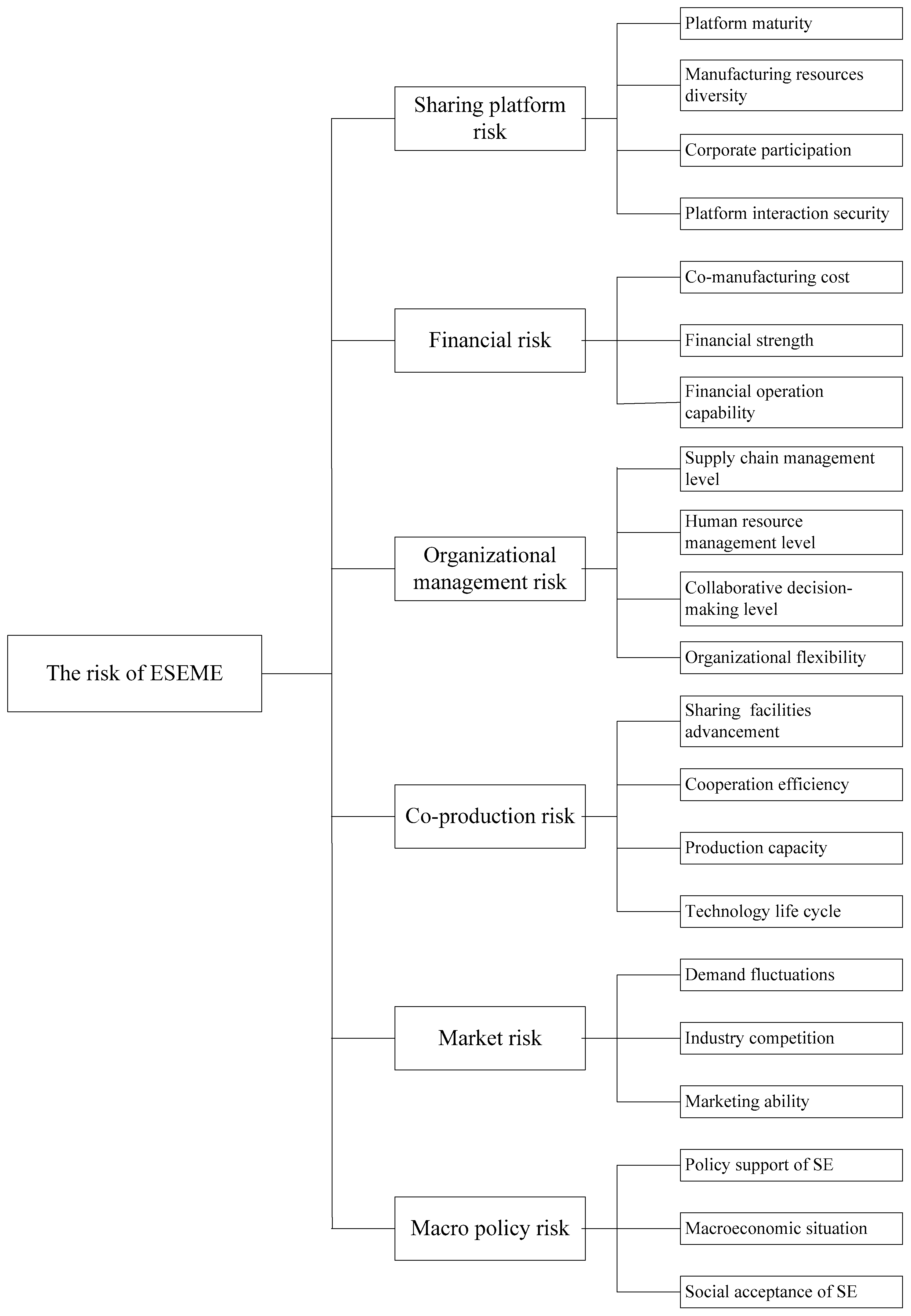
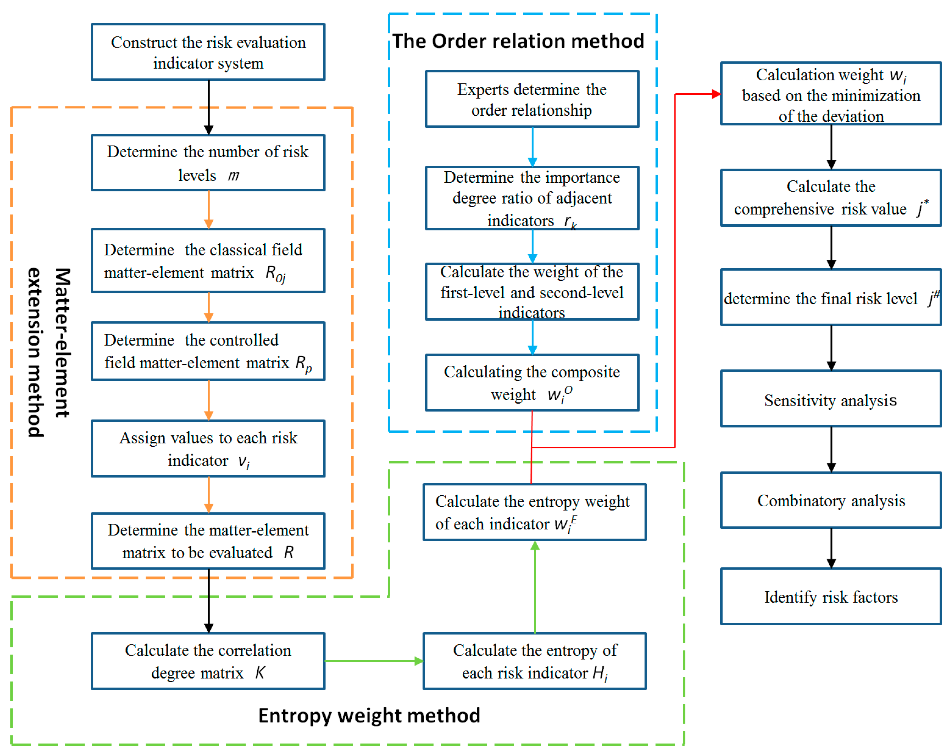
Based on the above studies, we introduce a matter–element extension based approach according to the characteristics of ESEME. The extension theory can be used to analyze and study the main risk indicators involved in the process of ESEME from the perspectives of sharing platform risk, financial risk, organizational management risk, co-production risk, market risk, and macro policy risk. Then, the matter–element extension model can be used to transform incompatible problems into compatible ones, so as to conduct risk assessment. However, different risk indicators may have different effects on the comprehensive risk value, so the weighting method of indicators is particularly important for risk assessment. The traditional matter–element model adopts a single subjective weighting method, and it has some limitations [49]. On the basis of the literature, methods used to weight assessment indicators are often AHP (Analytic Hierarchy Process), the entropy weight method, or a combination of AHP and the entropy weight method. The order relation method is a subjective weighting method that relies on the evaluators’ subjective attention to each indicator [50]. Compared with AHP, the order relation method is simpler and more practical, because it does not need to construct a judgment matrix and consistency test. Meanwhile, the entropy weight method is an objective weighting method, which determines indicators’ weights according to the variation degree of indicators’ values, and can effectively reflect the hidden information among indicators. Only the subjective weighting method or the objective weighting method is too one-sided in practical problems. Therefore, drawing upon the minimization of the deviation method, the comprehensive weight integrating entropy based weight and order relation based weight is obtained, and the risk level is determined. Next, by means of sensitivity analysis and combinatory analysis, sensitive risk indicators and the risk type of indicators can be identified.

The innovations of this paper are as follows:

(1).

According to a literature review, this is one of the first studies to assess the risk of ESEME. Unlike the existing risk research of the sharing economy, the matter–element extension method is adopted to construct a risk assessment indicator system for ESEME and more systematically assess the risk of ESEME.

(2).

On the basis of the traditional matter–element extension model, the method of indicator weighting is improved. We draw upon the minimum deviation method, which integrates the entropy weight method and the order relation method, and more reasonably reveal the importance of each risk indicator.

(3).

This work not only conducts a sensitivity analysis on the risk indicators’ values to identify risk indicators with high sensitivity, but also performs a combinatory analysis according to the comprehensive risk value and sensitivity, and then divides the risk indicators into four categories: Safety Type, Long-Term Planning Type, Preventive Type, and Critical Concern Type.

In summary, this paper constructs an effective and practical risk assessment model for ESEME. Through the model, the comprehensive risk value of a project can be obtained, and the risk factors with high sensitivity can be identified. Further, manufacturing enterprises can more accurately locate and control risk factors, and formulate more reasonable strategic planning.

2. Construction of the Risk Assessment Indicator System and the Matter–Element Extension Based Approach for ESEME

2.1. Risk Assessment Indicator System

In order to objectively assess the risk of ESEME, the relevant literature is reviewed widely first. According to the OECD/JRC Handbook, an indicator system should clearly define the object to be measured and its sub-components, and select appropriate indicators that reflect the dimensions of the overall composite and can be observed and measured [51]. From the perspective of sources, the risks faced by enterprises mainly come from themselves, the external environment, and partners [52]. As for enterprises themselves, there are mainly financial risks, and as for the external environment faced by the enterprises, there are mainly market risks [53]. Franks et al. [54] stated that environmental risks and social risks were critical factors that enterprises needed to consider. Based on the above research studies, this paper considers financial risk, market risk, and macro policy risk when first analyzing risk factors. According to the definition of the sharing economy, the sharing economy model consists of a sharing platform, demanders, and suppliers. Whether an enterprise can quickly find a matching supplier and successfully trade largely depends on the sharing platform, so the risk of the sharing platform is taken into account [13]. It is obviously one-sided to measure the internal risk of an enterprise only on financial risk, and the enterprise’s management and operation ability will also have an impact on the project, so the organizational management risk is worth paying attention to. In addition, an enterprise needs to interact and cooperate with a supplier, which is also an important part of ESEME, so co-production risk should also be taken into account. The establishment of an indicator system includes two aspects: the selection of indicators and the design of the indicator system structure. The selection of indicators should fully consider the concept and calculation range of each indicator, while the complexity of the multi-attribute comprehensive assessment often determines the hierarchical structure of the indicator system. As Olson, Birge, and Linton, three editors of the Technovation journal pointed out in the issue titled “Risk and Uncertainty Management in Technological Innovation”, risk linked to information technology should include unintended uses and threats both inside the enterprise [55] and along the supply chain [56], while risk associated with technology innovation should take marketing [57], supply chain partners [58], and other stakeholders [59] into consideration [60]. Based on the above theory and method of technical application risk, considering the characteristics of ESEME, we construct a risk assessment indicator system from six dimensions: sharing platform risk, financial risk, organizational management risk, co-production risk, market risk, and macro policy risk. The system includes six first-level indicators and 21 second-level indicators, as shown in Figure 1.

The corresponding symbols of the first-level indicators are given; sharing platform risk is expressed as $SPR$, financial risk is expressed as $FR$, organizational management risk is expressed as $OMR$, co-production risk is expressed as $CPR$, market risk is expressed as $MR$, and macro policy risk is expressed as $MPR$. According to the correlation between the indicators and the risk of ESEME, the 21 second-level indicators can be divided into two categories: forward indicators and reverse indicators. Forward indicators include demand fluctuations and industry competition, in which the higher the indicator’s value is, the higher the final risk will be, and the type is represented by “+”. For the remaining 19 indicators that are the reverse indicators, the higher the indicator’s value is, the lower the risk is, and the type is represented by “–”. The symbols, types, and explanation of the second-level indicators are shown in

Table 1. The symbols, types, and explanation of the second-level risk indicators.

Second-Level Indicator	Symbol	Type	Explanation
Platform maturity	$pm$	–	The degree to which users are satisfied with the sharing platform in terms of technology, design, functions, and services
Manufacturing resources diversity	$md$	–	The richness of the categories of manufacturing resources available for sharing
Corporate participation	$cp$	–	The degree of enthusiasm and initiative of manufacturing enterprises on the sharing platform
Platform interaction security	$is$	–	The reliability of the sharing platform to protect users’ information security and privacy
Co-manufacturing cost	$mc$	–	The degree to which the enterprise needs to provide production costs when cooperating with its supplier
Financial strength	$fs$	–	The richness of the enterprise’s funds
Financial operation capability	$fc$	–	The ability of the enterprise to handle capital turnover
Supply chain management level	$sl$	–	The overall efficiency and cost-effectiveness of the enterprise in supply chain
Human resource management level	$hl$	–	The level to manage employees in a scientific and rational way
Collaborative decision-making level	$dl$	–	The level of decision-making at which the enterprise and its supplier share information, resources, and conduct combat operations together
Organizational flexibility	$of$	–	The ability of the enterprise to face external changes without causing serious confusion in the organization
Sharing facilities advancement	$fa$	–	The ability of shared facilities to efficiently complete production tasks
Cooperation efficiency	$ce$	–	Productivity level of cooperation between the enterprise and its supplier
Production capacity	$pc$	–	The working ability of the enterprise’s employees
Technology life cycle	$tc$	–	The time course of production technology from research and development to elimination
Demand fluctuations	$df$	+	The degree of change in market demand for the enterprise’s products
Industry competition	$ic$	+	The position and pressure of the enterprise in the same industry
Marketing ability	$ma$	–	The ability of the enterprise to sell products
Policy support of SE	$ps$	–	Government’s support for the sharing economy business model
Macroeconomic situation	$ms$	–	The state of macroeconomic development of the country and its trends
Social acceptance of SE	$sa$	–	The public’s acceptance of the sharing economy business model

Note: “+” represented forward indicators; “–” represented reverse indicators.

.

2.2. The Matter–Element Extension Based Approach for ESEME

In the matter–element extension based approach, matter–element is the basic element describing objects, and it is an ordered triad composed of an object, characteristics, and the corresponding values of characteristics. Assuming that the risk of ESEME is $N$, the characteristic is $x$, and the value of the characteristic is $h$, then its matter–element can be expressed as $R=\left(N,x,h\right)$.

Firstly, the main characteristic matter–element matrix is defined. Assuming that the risk of ESEME $N$ has $s$ characteristics in total, and if there are $t$ main characteristics, then the main characteristic matter–element matrix of $N$ can be expressed as:

$$R=\left[\begin{array}{c}\begin{array}{ccc}N& x_1& h_1\end{array}\\ \begin{array}{ccc}& x_2& h_2\\ & ⋮& ⋮\\ & x_t& h_t\end{array}\end{array}\right]=\left[\begin{array}{c}{R}_1\\ R_2\\ \begin{array}{c}⋮\\ R_t\end{array}\end{array}\right]$$

(1)

where $R_i=\left(N,x_i,h_i\right)\left(i=1,2,\cdots ,t\right)$ represents the sub-characteristic matter–element matrix of $R$.

Secondly, the classical field matter–element matrix is defined. Suppose there are $m$ risk levels and $n$ risk indicators; then, the classical field matter–element matrix of the risk level $j\left(j=1,2,\cdots ,m\right)$ is expressed as:

$$R_{0j}=\left(N_{0j },c_i,v_{0ji }\right)=\left[\begin{array}{c}\begin{array}{ccc}{N}_{0j} & c_1& v_{0j1}\end{array}\\ \begin{array}{c}\begin{array}{cc} c_2& v_{0j2}\end{array}\\ \begin{array}{cc}⋮& ⋮\end{array}\\ \begin{array}{cc}{c}_n& v_{0jn}\end{array}\end{array}\end{array}\right]=\left[\begin{array}{c}\begin{array}{ccc}{N}_{0j} & c_1& \langle a_{0j1},b_{0j1}\rangle \end{array}\\ \begin{array}{c}\begin{array}{cc} c_2& \langle a_{0j2},b_{0j2}\rangle \end{array}\\ \begin{array}{cc}⋮& ⋮\end{array}\\ \begin{array}{cc}{c}_n& \langle a_{0jn},b_{0jn}\rangle \end{array}\end{array}\end{array}\right]$$

(2)

where $N_{0j}$ represents the $j\mathrm{th}$ risk level of ESEME; $c_i$ represents the $i$th $\left(i=1,2,\cdots ,n\right)$ risk indicator; $v_{0ji}$ represents the value range of $c_i$ on the $j\mathrm{th}$ risk level, expressed by $\langle a_{0ji},b_{0ji}\rangle$; $a_{0ji}$ represents the minimum value of $c_i$ on the $j\mathrm{th}$ risk level; and $b_{0ji}$ represents the maximum value of $c_i$ on the $j\mathrm{th}$ risk level.

Then, the controlled field matter–element matrix is defined.

$$R_p=\left(N_{p },c_i,v_{pi }\right)=\left[\begin{array}{c}\begin{array}{ccc}{N}_p & c_1& v_{p1}\end{array}\\ \begin{array}{c}\begin{array}{cc} c_2& v_{p2}\end{array}\\ \begin{array}{cc}⋮& ⋮\end{array}\\ \begin{array}{cc}{c}_n& v_{pn}\end{array}\end{array}\end{array}\right]=\left[\begin{array}{c}\begin{array}{ccc}{N}_p & c_1& \langle a_{p1},b_{p1}\rangle \end{array}\\ \begin{array}{c}\begin{array}{cc} c_2& \langle a_{p2},b_{p2}\rangle \end{array}\\ \begin{array}{cc}⋮& ⋮\end{array}\\ \begin{array}{cc}{c}_n& \langle a_{pn},b_{pn}\rangle \end{array}\end{array}\end{array}\right]$$

(3)

where $N_p$ represents the total risk level; $v_{pi}$ represents the corresponding value range of $c_i$ at the overall risk level, expressed by $\langle a_{pi},b_{pi}\rangle ; a_{pi}$ represents the minimum value of $c_i$ at the overall risk level; and $b_{pi}$ represents the maximum value of $c_i$ at the overall risk level.

Finally, the matter–element matrix to be evaluated is established.

$$R=\left(N_{ },c_i,v_{i }\right)=\left[\begin{array}{c}\begin{array}{ccc}N & c_1& v_1\end{array}\\ \begin{array}{c}\begin{array}{cc}{c}_2& v_2\end{array}\\ \begin{array}{cc}⋮& ⋮\end{array}\\ \begin{array}{cc}{c}_n& v_n\end{array}\end{array}\end{array}\right]$$

(4)

where $N$ represents the risk level to be identified; and $v_i$ represents the measured value of risk indicator $c_i$.

3. Assessment Methods

3.1. Correlation Degree Calculation Method

Since each risk indicator is a qualitative indicator, subjective valuation is required. The initial risk values of indicators are scored by experts from relevant fields, and the score range is [0, 100]. Then, the average of scores from all the experts is standardized, namely the measured values of risk indicators $v_i$. In order to calculate the correlation degree between each risk indicator and risk level, the concept of “proximity” is introduced here—that is, the quantitative relationship between the point and interval position. The calculation method of the proximity that each risk indicator to the classical field matter–element and the controlled field matter–element respectively is as follows:

$$\rho \left(v_i,v_{0ji}\right)=\left|v_i-\frac{a_{0ji}+b_{0ji}}{2}\right|-\frac{b_{0ji}-a_{0ji}}{2}$$

(5)

$$\rho \left(v_i,v_{pi}\right)=\left|v_i-\frac{a_{pi}+b_{pi}}{2}\right|-\frac{b_{pi}-a_{pi}}{2}$$

(6)

$$i=1,2,\cdots ,n;j=1,2,\cdots ,m$$

where $\rho \left(v_i,v_{0ji}\right)$ represents the proximity of the $i$th risk indicator to the corresponding classical field matter–element at the $j\mathrm{th}$ risk level; and $\rho \left(v_i,v_{pi}\right)$ represents the proximity of the $i$th risk indicator to the corresponding controlled field matter–element at the $j\mathrm{th}$ risk level.

Then, the correlation degree between the $i$th risk indicator and the $j\mathrm{th}$ risk level can be expressed as:

$$K_j\left(v_i\right)=\{\begin{array}{c}\frac{-\rho \left(v_i,v_{0ji}\right)}{\left|v_{0ji}\right|} , v_i\in v_{0ji}\\ \frac{\rho \left(v_i,v_{0ji}\right)}{\rho \left(v_i,v_{pi}\right)-\rho \left(v_i,v_{0ji}\right)}, v_i\notin v_{0ji}\end{array}$$

(7)

When the correlation degree of each indicator and each risk level is obtained, the correlation degree matrix can be expressed as $K={\left[K_j\left(v_i\right)\right]}_{n\times m}$.

3.2. Comprehensive Weighting Method

3.2.1. Entropy Weight Method

As far as we know, entropy can be used to measure the disorder degree of a system [61]. The smaller the entropy value is, the more effective information the system contains, and the more important this characteristic is. Therefore, entropy weight can be considered to determine the weight of risk indicators. The entropy weight method is already a mature objective weighting method that is widely used in many fields. For instance, Xu et al. [62] used the improved entropy weight method to determine the weight of each assessment indicator for urban flooding risk assessment. Liu et al. [63] also uses the entropy weight method when conducting fire risk assessment for large-scale commercial buildings. In order to assess concentrated solar power technologies, Cavallaro et al. [64] proposed a modified intuitionistic fuzzy TOPSIS with a trigonometric entropy vector weight method. Based on the matter–element extension model, the entropy weight of each risk indicator is determined. The main calculation steps are as follows:

(1).

Calculate the correlation degree $K_j\left(v_i\right)$ between the measured value $v_i$ of the risk indicator $c_i$ and the $j\mathrm{th}$ risk level according to the Formulas (5)–(7), and then construct the correlation degree matrix $K={\left(r_{ij}\right)}_{n\times m}$, where $r_{ij}$ = $K_j\left(v_i\right),\left(j=1,2,\cdots ,m, i=1,2,\cdots ,n\right)$.

(2).

Calculate the entropy value of each risk indicator, and the calculate formula is as follows:

$$H_i=-k{\displaystyle \sum }_{j=1}^m{f}_{ij}·\ln f_{ij}$$

(8)

where:

$$k=\frac{1}{\ln m},$$

$$f_{ij}=\frac{r_{ij}}{{{\displaystyle \sum }}_{j=1}^m{r}_{ij}}$$

If the correlation degree $r_{ij}=0$, then $\ln f_{ij}$ is meaningless; to avoid this problem, the calculation method of $f_{ij}$ needs to be corrected. The correction result is as follows:

$$f_{ij}=\frac{1+r_{ij}}{{{\displaystyle \sum }}_{j=1}^m\left(1+r_{ij}\right)}$$

(3).

Determine the entropy weight of each risk indicator, which is calculated as follows:

$$w_i^E=\frac{1-H_i}{n-{{\displaystyle \sum }}_{i=1}^n{H}_i}$$

(9)

3.2.2. The Order Relation Method

The order relation method is a subjective weighting method that is based on the expert’s importance ranking and quantitative assignment of assessment indicators. In this method, it is not necessary to construct a judgment matrix and consistency test, and the calculation is relatively simple. The steps of determining the weight of risk indicators by the order relation method are as follows:

(1).

Determine the order relationship. Supposing that the importance of the assessment indicator $x_i$ is not less than $x_j$, it is denoted as $x_i>x_j$. At the beginning, the relevant experts select the most important one from the assessment indicators set $\left\{x_1,x_2,\cdots ,x_n\right\}$, which is marked as $x_1{}^{*}$. Then, experts select the most important one of the remaining $n-1$ evaluation indicators, which is marked as $x_2{}^{*}$. In a similar way, until the end of the sort, we get the order relationship $x_1{}^{*}>x_2{}^{*}>\cdots >x_n{}^{*}$.

(2).

Determine the importance degree ratio of adjacent indicators. The expert gives the ideal judgment of the importance degree ratio $w_{k-1}^O/w_k^O$ of the adjacent indicators $x_{k-1}$ and $x_k$ as:

$$\frac{w_{k-1}^O}{w_k^O}=r_k, \left(k=n,n-1,n-2,\cdots ,3,2\right)$$

(10)

The value of $r_k$ can be referred to

Table 2. $r_k$ assignment reference table.

${\mathit{r}}_{\mathit{k}}$	Explanation
1.0	Indicator $x_{k-1}$ is as important as the indicator $x_k$
1.2	Indicator $x_{k-1}$ is a little more important than the indicator $x_k$
1.4	Indicator $x_{k-1}$ is obviously more important than the indicator $x_k$
1.6	Indicator $x_{k-1}$ is strongly more important than the indicator $x_k$
1.8	Indicator $x_{k-1}$ is extremely more important than the indicator $x_k$

.

(3).

Calculate the weight coefficient $w_i^O$. Suppose the $r_k$ given by the experts satisfies the constraint $r_{k-1}>1/r_k,\left(k=n,n-1,n-2,\cdots ,3,2\right)$; then, $w_k$ is:

$$w_n^O={\left(1+{\displaystyle \sum }_{k=2}^n{\displaystyle \prod }_{i=k}^n{r}_i\right)}^{-1}$$

(11)

$$w_{k-1}^O=r_k{w}_k^O,\left(k=n,n-1,n-2,\cdots ,3,2\right)$$

(12)

3.2.3. Minimum Deviation Weight

Combined with the idea of optimization theory, different methods are used to determine the weights of the risk indicators of ESEME, and construct a basic weight vector $w_t=\left\{w_{t1},w_{t2},\cdots ,w_{tn}\right\}\left(t=1,2,\cdots ,T\right)$; then, any linear combination of $T$ weight vectors is:

$$w^{*}={\displaystyle \sum }_{t=1}^T{\alpha }_t·w_t{}^T,{\alpha }_t>0$$

(13)

Then, based on the idea of minimization of deviation, the linear combination coefficient ${\alpha }_t$ in Equation (13) is optimized, and the most satisfactory weight vector $w$ is selected, which includes the minimum deviation weights. The decision model is as follows:

$$\min ||{\displaystyle \sum }_{t=1}^T{\alpha }_t·w_t{}^T-w_i{}^T{\left|\right|}_2,\left(i=1,2,\cdots ,T\right)$$

(14)

In the process of risk assessment, in order to avoid the one-sidedness of the indicators’ weights, this paper comprehensively considered the entropy weight method belonging to the objective weighting method and the order relation method belonging to the subjective weighting method, and determined the final risk indicators’ weights through the optimization idea of minimum deviation.

3.3. Comprehensive Risk Value Calculation Method

Firstly, after determining the comprehensive weights of the risk indicators, it can be known that the comprehensive correlation degree of the risk $N$ to be evaluated with the $j\mathrm{th}$ risk level is:

$$K_j\left(N\right)={\displaystyle \sum }_{i=1}^n(w_i·K_j\left(v_i\right)),j=1,2,\cdots ,m$$

(15)

where ${\sum }_{i=1}^n{w}_i=1$.

Secondly, suppose that $K_{j^{\#}}\left(N\right)=\max \left(K_j\left(N\right)\right)$; then, the overall risk level is $j^{\#}$.

Then, calculate the risk value $j^{*}$ of ESEME. The calculation formula is as follows:

$$\overline{K_j}\left(N\right)=\frac{K_j\left(N\right)-\min K_j\left(N\right)}{\max K_j\left(N\right)-\min K_j\left(N\right)},j=1,2,\cdots ,m$$

(16)

$$j^{*}=\frac{{\sum }_{j=1}^m\left(j·\overline{K_j}\left(N\right)\right)}{{\sum }_{j=1}^m\overline{K_j}\left(N\right)}$$

(17)

where $\min K_j\left(N\right)$ represents the minimum risk level correlation, and $\max K_j\left(N\right)$ represents the maximum risk level correlation.

3.4. Sensitivity Analysis

As Saltelli et al. noted in the global sensitivity analysis [65], “Careful use of experimental designs can often answer more specific questions, with an investment of few resources”. In the ESEME context, there is no trial-and-error condition, and enterprises do not want to see the actual risk and loss occur. Consequently, the numerical experimental design method is adopted to analyze the sensitivity of all the indicators. During experiments, some variables can be controlled (e.g., temperature, duration), while some variables cannot be controlled but can affect experimental results (e.g., air pressure and humidity). More importantly, the purpose of experiments is to observe the characteristics of each variable affecting one or more measurements. Specifically, the sensitivity of each risk indicator is observed by changing the value of each risk indicator according to the absolute value and the ratio, and measuring the total risk value after the change. Similar sensitivity analysis methods to observe changes of target variables by adjusting indicators’ values have been applied in matter–element analysis; for example, He et al. conducted sensitivity analysis on the value and weight of urban grid planning risk indicators [66]. Li and Peng introduced sensitivity analyses to reveal the influence of the change of indicators’ values on each indicator’s weight and the eigenvalue of the grade, and to find out the main impact indicators [49]. To implement sensitivity analysis, the key indicator and corresponding influencing factors should be determined firstly. Under the same conditions, change the values of relevant factors one by one and observe the changing laws of the key indicator through the objective function to identify the sensitive factors. Suppose there are $n$ influencing factors whose values are $x_1,x_2,\cdots ,x_n$ respectively; then, the value of the objective function is $y\left(x\right)=\left(x_1,x_2,\cdots ,x_n\right)$, and the value of the function after the change of the $i\mathrm{th}\left(i=1,2,\cdots ,n\right)$ factor value is $y\left(x_{ij}\right)$. After $t$ tests, the sensitivity of the factor can be expressed as:

$${\sigma }_i=\sqrt{\frac{1}{t-1}{\displaystyle \sum }_{j=1}^t{\left[y\left(x_{ij}\right)-{\mu }_i\right]}^2},j=1,2,\cdots ,t$$

(18)

where ${\mu }_i=\frac{1}{t}{\sum }_{j=1}^{t}y\left(x_{ij}\right)$.

From the above calculation, the larger the $\sigma$ of a factor, the stronger the sensitivity. Ranking sensitivities of factors, sensitive factors that have a greater impact on the key indicator can be identified. In order to more intuitively and clearly learn the sensitivity of each influencing factor, it can also be presented by means of charts.

3.5. Combinatory Analysis

Combinatory analysis requires a coordinate system, where risk indicators’ values and their corresponding sensitivities can be inserted. According to the average value of each indicator’s sensitivity $\overline{\sigma }$ and the average value of each indicator $\overline{x}$, the coordinate system can be divided. For the relationship of each indicator’s value $x_i$ and sensitivity ${\sigma }_i$—that is, the distribution position in the coordinate system—the risk indicators can be divided into four types.

The first type is called the “Safety Type”. The indicator’s value and sensitivity of this type are low $\left(x_i\le \overline{x} \& {\sigma }_i\le \overline{\sigma }\right)$, which has less impact on the comprehensive risk and does not have to be too concerned.

The second type is called the “Long-Term Planning Type”. Such risk indicators have higher values but lower sensitivity $\left(x_i>\overline{x} \& {\sigma }_i\le \overline{\sigma }\right)$. Even if the indicator’s value decreases in the short term, it has little effect on the comprehensive risk. Therefore, the risk indicators of this type need long-term continuous control at a certain level.

The third type is called the “Preventive Type”. The indicator’s value of such risk indicators are low, but its sensitivity is very high $\left(x_i\le \overline{x} \& {\sigma }_i>\overline{\sigma }\right)$. However, the fluctuation of the indicator’s value may cause great change in the comprehensive risk value. Therefore, such indicators need to be defended in advance and measures need to be taken to keep their values low.

The fourth type is called the “Critical Concern Type”. The indicator’s value and sensitivity of such risk indicators are very high $\left(x_i>\overline{x} \& {\sigma }_i>\overline{\sigma }\right)$. Although the indicator’s value changes slightly, it may lead to significant change in the comprehensive risk value. If such indicators are effectively managed, the comprehensive risk value can be significantly reduced. However, if they are not managed properly, the comprehensive risk value may rise sharply. Therefore, it is necessary to pay special attention to these indicators.

3.6. Assessment Process

The risk assessment process of ESEME based on the matter–element extension method is as follows.

Step 1

Construct a risk assessment indicator system that is suitable for ESEME.

Step 2

Determine the number of risk levels $m$, the classical field matter–element matrix $R_{0j}$, and the controlled field matter–element matrix $R_p$ of each risk level.

Step 3

Assign values to each risk indicator and determine the matter–element matrix to be evaluated, $R$.

Step 4

Calculate the correlation degree $K_j\left(v_i\right)$ between each risk indicator and each risk level, and form the correlation degree matrix $K$.

Step 5

Calculate the entropy weight $w_i^E$ of each indicator according to the correlation degree matrix.

Step 6

Determine the subjective weight $w_i^O$ of each indicator based on the order relation method.

Step 7

Determine the comprehensive weight $w_i$ based on the idea of minimization of deviation.

Step 8

Calculate the comprehensive risk value $j^{*}$ of ESEME and determine the final risk level $j^{\#}$.

Step 9

Conduct sensitivity analysis and combinatory analysis to identify risk factors.

The assessment process of comprehensive risk is shown in Figure 2.

4. Example Analysis

E is a small and medium-sized manufacturing enterprise in China, which is committed to expanding its production scale and improving its sales performance. Due to insufficient internal funds and incomplete production facilities, enterprise E plans to engage in the sharing economy to solve existing issues in a low-cost way. Based on the matter–element extension method and the minimum deviation weighting method, this paper studies the risk issues of enterprise E engaging in the sharing economy. In order to assess the risks of enterprise E, an assessment group is formed, which consists of professors, associate professors, and doctoral students engaged in research related to the sharing economy and risk assessment, as well as manufacturing enterprise engineers and department managers, respectively from our university, enterprise E, and another manufacturing enterprise. Then, enterprise E provides detailed information on its business conditions, technical strengths, and progress on engagement in the sharing economy, and the assessment group evaluates indicators according to the risk indicator system in Section 2.1. By the way, it is understandable that different experts have different opinions. On this basis, the paper implements a risk assessment of enterprise E’s engagement in the sharing economy according to the assessment process in Section 3.6. The specific steps are as follows.

4.1. Calculation of Risk Value

4.1.1. Determination of the Matter–Element Matrices

The risk levels are divided into four categories, which are low, medium–low, medium–high, and high. According to the value range of each risk indicator $c_i\left(i=1,2,\cdots ,21\right)$ in different risk levels, the classical field matter–element matrix and the controlled field matter–element matrix are determined successively.

The classical field matter–element matrix is:

$$R_{01}=\left[\begin{array}{c}\begin{array}{ccc}{N}_{01} & c_1& \langle 0,0.25\rangle \end{array}\\ \begin{array}{c}\begin{array}{cc} c_2& \langle 0,0.25\rangle \end{array}\\ \begin{array}{cc}⋮& ⋮\end{array} \\ \begin{array}{cc} c_{21}& \langle 0,0.25\rangle \end{array}\end{array}\end{array}\right]$$

$$R_{02}=\left[\begin{array}{c}\begin{array}{ccc}{N}_{02} & c_1& \langle 0.25,0.5\rangle \end{array}\\ \begin{array}{c}\begin{array}{cc} c_2& \langle 0.25,0.5\rangle \end{array}\\ \begin{array}{cc}⋮& ⋮\end{array} \\ \begin{array}{cc} c_{21}& \langle 0.25,0.5\rangle \end{array}\end{array}\end{array}\right].$$

$$R_{03}=\left[\begin{array}{c}\begin{array}{ccc}{N}_{03} & c_1& \langle 0.5,0.75\rangle \end{array}\\ \begin{array}{c}\begin{array}{cc} c_2& \langle 0.5,0.75\rangle \end{array}\\ \begin{array}{cc}⋮& ⋮\end{array} \\ \begin{array}{cc} c_{21}& \langle 0.5,0.75\rangle \end{array}\end{array}\end{array}\right]$$

$$R_{04}=\left[\begin{array}{c}\begin{array}{ccc}{N}_{04} & c_1& \langle 0.75,1\rangle \end{array}\\ \begin{array}{c}\begin{array}{cc} c_2& \langle 0.75,1\rangle \end{array}\\ \begin{array}{cc}⋮& ⋮\end{array} \\ \begin{array}{cc} c_{21}& \langle 0.75,1\rangle \end{array}\end{array}\end{array}\right]$$

The controlled field matter–element matrix is:

$$R_p=\left[\begin{array}{c}\begin{array}{ccc}{N}_p & c_1& \langle 0,1\rangle \end{array}\\ \begin{array}{c}\begin{array}{cc} c_2& \langle 0,1\rangle \end{array}\\ \begin{array}{cc}⋮& ⋮\end{array}\\ \begin{array}{cc}{c}_{21}& \langle 0,1\rangle \end{array}\end{array}\end{array}\right]$$

Since each risk indicator is a qualitative indicator, subjective valuation is required. Five experts are invited to score each risk indicator, and the score range is [0, 100]. Then, the average of the five scores is standardized (see Appendix A). The final matter–element matrix to be evaluated is:

$$R=\left[\begin{array}{ccc}N& C_1& 0.444\\ & C_2& 0.506\\ & C_3& 0.764\\ & C_4& 0.418\\ & C_5& 0.270\\ & C_6& 0.382\\ & C_7& 0.502\\ & C_8& 0.318\\ & C_9& 0.346\\ & C_{10}& 0.494\\ & C_{11}& 0.688\\ & C_{12}& 0.292\\ & C_{13}& 0.814\\ & C_{14}& 0.344\\ & C_{15}& 0.280\\ & C_{16}& 0.480\\ & C_{17}& 0.758\\ & C_{18}& 0.262\\ & C_{19}& 0.238\\ & C_{20}& 0.378\\ & C_{21}& 0.410\end{array}\right]$$

4.1.2. Calculation of the Correlation Degree Matrix

Calculate the correlation degree between each risk indicator and each risk level according to Formulas (5)–(7). The correlation degree matrix $K$ is:

$$K={\left[K_j\left(v_i\right)\right]}_{21\times 4}=\left[\begin{array}{cccc}-0.3041& 0.2240& -0.1120& -0.4080\\ -0.3413& -0.0120& 0.0240& -0.3306\\ -0.6853& -0.5280& -0.0560& 0.0560\\ -0.2867& 0.3280& -0.1640& -0.4427\\ -0.0690& 0.0800& -0.4600& -0.6400\\ -0.2568& 0.4720& -0.2360& -0.4907\\ -0.3360& -0.0040& 0.0080& -0.3324\\ -0.1762& 0.2720& -0.3640& -0.5760\\ -0.2172& 0.3840& -0.3080& -0.5387\\ -0.3306& 0.0240& -0.0120& -0.3413\\ -0.5840& -0.3760& 0.2480& -0.1658\\ -0.1257& 0.1680& -0.4160& -0.6107\\ -0.7520& -0.6280& -0.2560& 0.2560\\ -0.2146& 0.3760& -0.3120& -0.5413\\ -0.0968& 0.1200& -0.4400& -0.6267\\ -0.3239& 0.0800& -0.0400& -0.3600\\ -0.6773& -0.5160& -0.0320& 0.0320\\ -0.0438& 0.0480& -0.4760& -0.6507\\ 0.0480& -0.0480& -0.5240& -0.6827\\ -0.2530& 0.4880& -0.2440& -0.4960\\ -0.2807& 0.3600& -0.1800& -0.4533\end{array}\right]$$

(19)

4.1.3. Calculation of Indicator’s Weight

First of all, for determining the weight of the first-level risk indicators based on the order relation method, five experts are invited again to rank the importance of the first-level risk indicators, and the importance degree ratio of the adjacent indicators is determined according to Table 2. Then, the weight of each first-level risk indicator is calculated according to Formulas (11) and (12), and the average value of the weights obtained by the five experts is taken. Similarly, the weights of all the second-level indicators below each first-level indicator are calculated, respectively. The indicators’ order relationship, the importance ratio between the two adjacent indicators and indicators’ weights from the five experts are provided in Appendix B. Then, the weight of the second-level indicator is multiplied by the weight of the first-level indicator to which it belongs, which is the combined weight of the second-level indicator based on the order relation method. Afterwards, the entropy weight is obtained according to the correlation degree matrix $K$ and the calculation steps shown in Section 3.2.1. Then, the minimum deviation weight is calculated through the Formulas (13) and (14), which is the comprehensive weight required in this paper. Ultimately, the indicators’ comprehensive weights are shown in

Table 3. Comprehensive weight based on minimization of deviation.

First-Level Indicator	Weight	Second-Level Indicator	Weight	Combined Weight	Entropy Weight	Comprehensive Weight
$SPR$	0.2618	$pm$	0.2522	0.0660	0.0255	0.0487
		$md$	0.2961	0.0775	0.0139	0.0504
		$cp$	0.2828	0.0740	0.0688	0.0718
		$is$	0.1689	0.0442	0.0351	0.0403
$FR$	0.3234	$mc$	0.3489	0.1128	0.0544	0.0879
		$fs$	0.3614	0.1169	0.0520	0.0892
		$fc$	0.2897	0.0937	0.0134	0.0595
$OMR$	0.0991	$sl$	0.3179	0.0315	0.0505	0.0396
		$hl$	0.1818	0.0180	0.0524	0.0327
		$dl$	0.3289	0.0326	0.0139	0.0246
		$of$	0.1715	0.0170	0.0504	0.0312
$CPR$	0.0984	$fa$	0.1999	0.0197	0.0510	0.0331
		$ce$	0.2909	0.0286	0.1156	0.0657
		$pc$	0.2963	0.0292	0.0522	0.0390
		$tc$	0.2129	0.0209	0.0524	0.0343
$MR$	0.0988	$df$	0.3645	0.0360	0.0162	0.0276
		$ic$	0.3013	0.0298	0.0653	0.0449
		$ma$	0.3342	0.0330	0.0566	0.0431
$MPR$	0.1186	$ps$	0.3808	0.0452	0.0676	0.0548
		$ms$	0.3375	0.0400	0.0542	0.0460
		$sa$	0.2817	0.0334	0.0385	0.0356

.

4.1.4. Calculation of the Comprehensive Risk Value

According to Formula (15), the correlation degree between the risk of ESEME and each risk level can be calculated, which is $K_1\left(N\right)=-0.3077, K_2\left(N\right)=0.0435, K_3\left(N\right)=-0.2201$, and $K_4\left(N\right)=-0.3830$, respectively. From the above calculation results, we can know that the value of $K_2\left(N\right)$ is the largest, so the risk level of ESEME is medium–low. According to Formulas (16) and (17), the final risk value of ESEME can be calculated as 2.1317.

4.2. Analysis of Calculation Results

According to the comprehensive risk value 2.1317, the overall risk of enterprise E is medium–low, indicating that enterprise E will encounter a little risk resistance in the process of engagement in the sharing economy. From the correlation degree matrix, the risk level of each second-level risk indicator can be known. Among all the 21 risk indicators, only $ps$ (Policy support of SE) is at a low risk level, which means that enterprise E can get support from the government when they engage in the sharing economy, and it is conducive to its sustainable development. Fourteen indicators are at a medium–low risk level, respectively $pm$ (Platform maturity), $is$ (Platform interaction security), $mc$ (Co-manufacturing cost), $fs$ (Financial strength), $sl$ (Supply chain management level), $hl$ (Human resource management level), $dl$ (Collaborative decision-making level), $fa$ (Sharing facilities advancement), $pc$ (Production capacity), $tc$ (Technology life cycle), $df$ (Demand fluctuations), $ma$ (Marketing ability), $ms$ (Macroeconomic situation), and $sa$ (Social acceptance of SE). Although the current risks are small, these indicators remain to be seen, because they may become medium–high risk or high risk as environmental changes. Three indicators are at the medium–high risk level; these are respectively $md$ (Manufacturing resources diversity), $fc$ (Financial operation capability), and $of$ (Organizational flexibility). Three indicators are also at the high level, which are $cp$ (Corporate participation), $ce$ (Cooperation efficiency), and $ic$ (Industry competition). They require special attention, and enterprise E needs to control and prevent for different risk factors.

In addition to judging the risk level of the second-level risk indicators and calculating the comprehensive risk value, the risk level of the six first-level indicators can also be judged according to Formula (15). Since $K_1\left(SPR\right)=0.0502$ is the largest among $K_j\left(SPR\right)\left(j=1,2,3,4\right)$, the sharing platform risk is at a low level; Since $K_3\left(FR\right)=0.0350$ is the largest among $K_j\left(FR\right)$, the financial risk is at a medium-high level. Since $K_1\left(OMR\right)=0.0103$ is the largest among $K_j\left(OMR\right)$, the organizational management risk is at a low level. Since $K_2\left(CPR\right)=0.0141$ is the largest among $K_j\left(CPR\right)$, the co-production risk is at a medium–low level. Since $K_2\left(MR\right)=0.0132$ is the largest among $K_j\left(MR\right)$, the market risk is at a medium–low level. Since $K_2\left(MPR\right)=0.0026$ is the largest among $K_j\left(MPR\right)$, the macro policy risk is at a medium–low level. Then, enterprise E could adjust the corresponding departments’ work according to the risk levels of first-level indicators.

4.3. Sensitivity Analysis

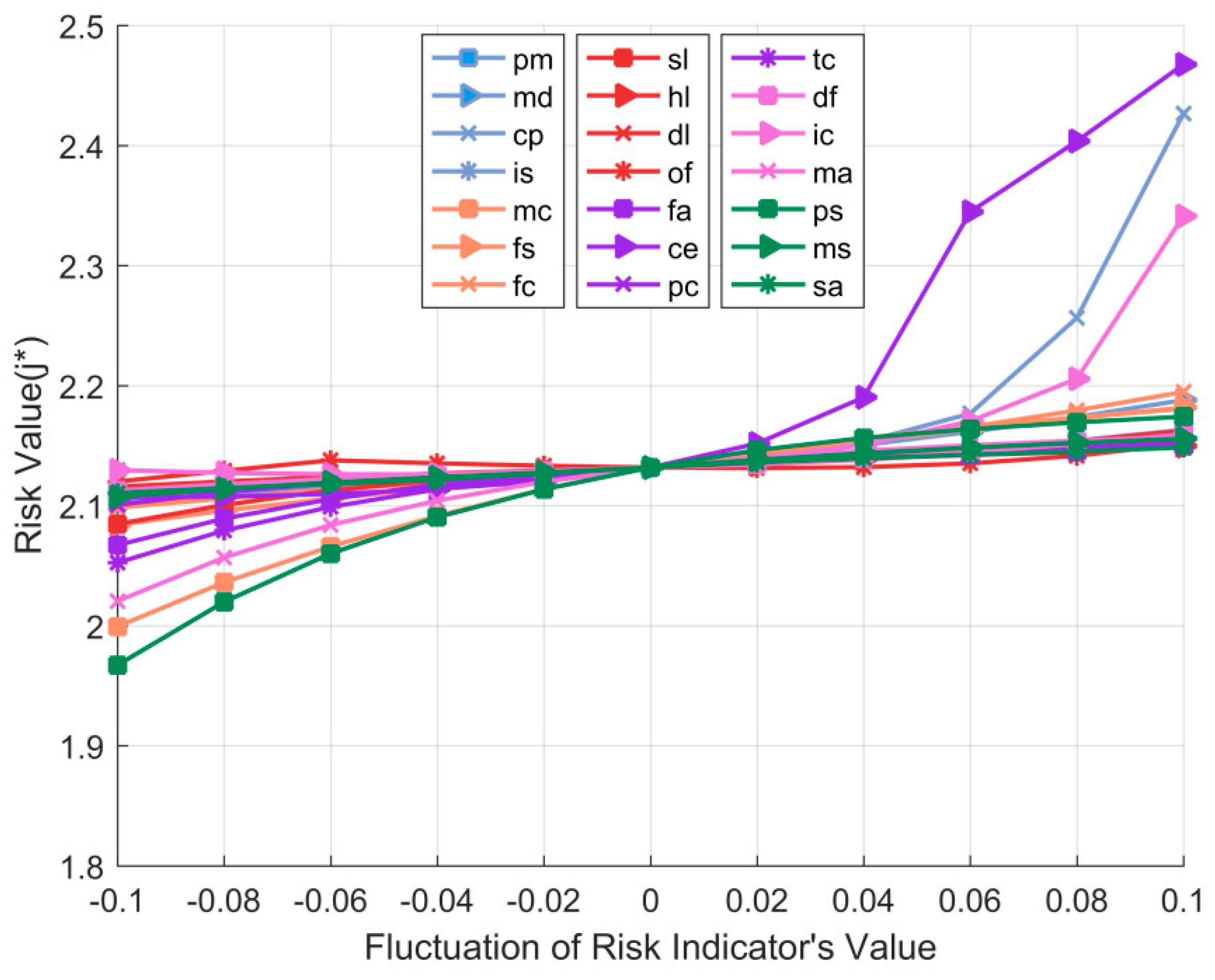
In order to observe the influence of the final risk value when the indicator’s value changes and identify the sensitive risk factors, a sensitivity analysis on the risk indicator’s value is implemented. When the value of a single indicator changes by ±0.1, the corresponding risk value changes are shown in Figure 3.

According to the sensitivity analysis of the indicators’ values, the six most sensitive indicators are $ce$ (Cooperation efficiency), $cp$ (Corporate participation), $ps$ (Policy support of SE), $ic$ (Industry competition), $mc$ (Co-manufacturing cost), and $ma$ (Marketing ability). As can be seen from Figure 3, when the value of $ce$ (Cooperation efficiency) increases by 0.04–0.1, the comprehensive risk value rises sharply; when the value of $cp$ (Corporate participation) or $ic$ (Industry competition) increases by 0.06–0.1, the comprehensive risk value rises significantly. What’s more, when the value of $mc$ (Co-manufacturing cost), $ma$ (Marketing ability), or $ps$ (Policy support of SE) is gradually reduced by 0.1, the comprehensive risk value slowly decreases. Therefore, in order to prevent the increase of the comprehensive risk value, it is necessary to focus on $ce$ (Cooperation efficiency), $cp$ (Corporate participation), and $ic$ (Industry competition). Assuming that the comprehensive risk value needs to be reduced, enterprise E can reduce the co-manufacturing cost, improve the marketing ability, and increase the policy support of SE.

In addition, sensitivity analyses of the comprehensive risk value based on the order relation weighting method and entropy weight method are also carried out under the same conditions. When weighting based on the order relation method, the result shows that the comprehensive risk value changes linearly with the change of a single indicator’s value. For example, with the continuous increase of $mc$ (Co-manufacturing cost), the comprehensive risk value increases linearly, while with the continuous increase of $cp$ (Corporate participation), the comprehensive risk value decreases linearly. However, this phenomenon indicates the limitation of the assessment of the matter–element extension model based on the single order relation method. While the variation trend of the comprehensive risk value based on the entropy weight method is similar to that in Figure 3, the variation range of the comprehensive risk value is larger than that in Figure 3, and there are differences in the details. Since the entropy weight method is an objective weighting method, which relies on objective data and in this paper depends on the correlation degree obtained by the matter–element extension model, it is unreasonable to assess the risk of enterprise E engaging in the sharing economy based on the entropy weight method alone.

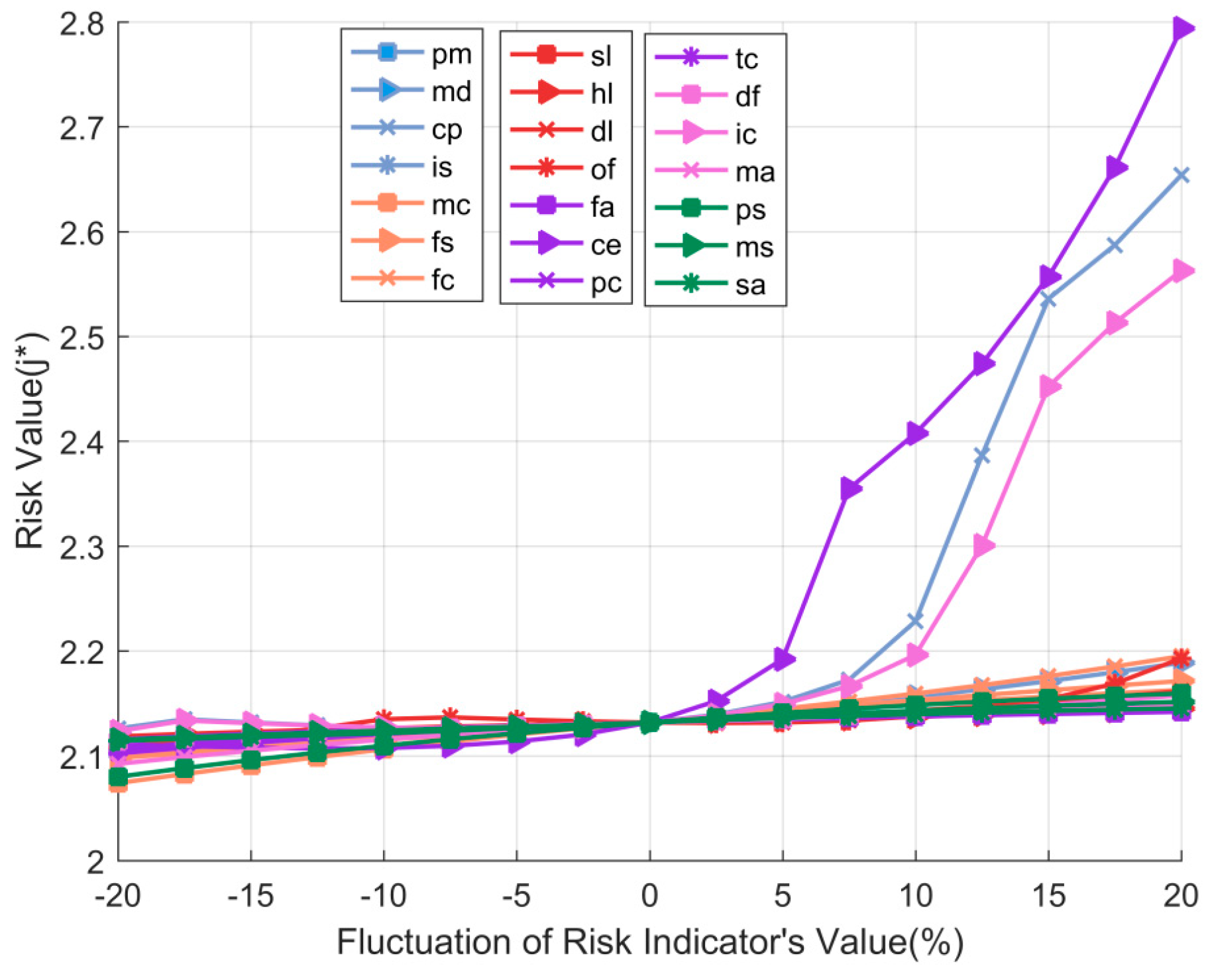
Due to there being large differences in values of these indicators, the results calculated by increasing or decreasing the fixed value will be biased. In order to eliminate this deviation, a sensitivity analysis on the comprehensive risk value when the indicator’s value changes ±20% is implemented, and the results are shown in Figure 4. Under the same conditions, sensitivity analyses of the comprehensive risk value based on the order relation weighting method and entropy weight method are also implemented.

According to the analysis results, the six most sensitive indicators are $ce$ (Cooperation efficiency), $cp$ (Corporate participation), $ic$ (Industry competition), $fc$ (Financial operation capability), $mc$ (Co-manufacturing cost), and $md$ (Manufacturing resources diversity). Among them, the high sensitivity of $cp$ (Corporate participation), $ce$ (Cooperation efficiency), or $ic$ (Industry competition) benefits from its high value, which requires focus. Although the value of $md$ (Manufacturing resources diversity), $mc$ (Co-manufacturing cost), or $fc$ (Financial operation capability) is not high, they are also worthy of attention. Weighting based on the order relation method, the result shows that the comprehensive risk value decreases with the increase of some indicators’ values. Obviously, the matter–element extension model based on the order relation method alone is not reasonable. Further, the variation trend of the comprehensive risk value based on the entropy weight method is similar to that in Figure 4, but the variation range of the comprehensive risk value is larger than that in Figure 4, and there are subtle differences in the sensitivities of some indicators.

4.4. Combinatory Analysis

In order to further study the relationship between a risk indicator’s value and sensitivity, a combinatory analysis is implemented.

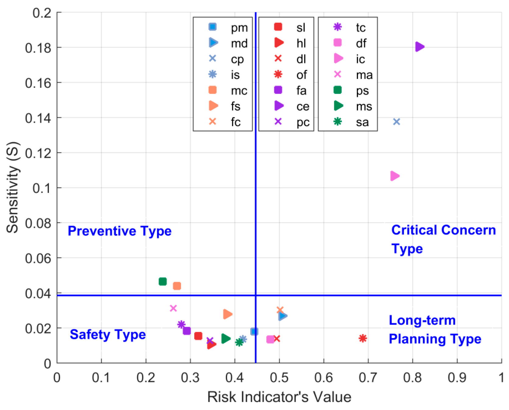
In Figure 5, the horizontal axis represents the standardized indicator’s value evaluated by experts, and the vertical axis represents the average standard deviation of the risk indicator’s value changes by ±0.1 and ±20%, namely the comprehensive sensitivity of the indicator’s value. According to the distribution position of each risk indicator in the coordinate system, the types of the 21 risk indicators are determined as follows.

The “Safety Type” includes $pm$ (Platform maturity), $is$ (Platform interaction security), $fs$ (Financial strength), $sl$ (Supply chain management level), $hl$ (Human resource management level), $fa$ (Sharing facilities advancement), $pc$ (Production capacity), $tc$ (Technology life cycle), $ma$ (Marketing ability), $ms$ (Macroeconomic situation), and $sa$ (Social acceptance of SE); these risk indicators have little effect on the overall risk value.

The “Long-term Planning Type” includes $df$ (Demand fluctuations), $dl$ (Collaborative decision-making level), $fc$ (Financial operation capability),$md$ (Manufacturing resources diversity), and $of$ (Organizational flexibility). Such risk indicators have higher value, but lower sensitivity. Even if the indicator’s value changes in the short term, it will have little effect on the comprehensive risk value.

The “Preventive Type” includes $mc$ (Co-manufacturing cost) and $ps$ (Policy support of SE). The fluctuations of these indicators’ values may lead to large changes in the comprehensive risk value, so enterprise E needs to take measures to keep the co-manufacturing cost at a low level in advance, and strives to get the government’s support.

The “Critical Concern Type” includes $ce$ (Cooperation efficiency), $cp$ (Corporate participation), and $ic$ (Industry competition). For such indicators, a slight change of their values may lead to a significant change in the comprehensive risk value, so enterprise E needs to pay close attention to these indicators.

5. Discussion and Implications

In order to study the risk of ESEME, this paper constructs the risk assessment indicator system of ESEME by referring to the existing literature. Then, the matter–element extension model is introduced, and the risk of enterprise E engaging in the sharing economy is assessed based on the minimum deviation weight. The assessment results include a precise risk value and the risk level, which are recognized by the experts who have previously given the risk value and weights of the indicators. In addition, highly sensitive indicators are found through sensitivity analysis, which provides a basis for small and medium-sized manufacturing enterprises to accurately identify high-risk factors. By combinatory analysis, all the risk indicators are divided into four risk types, which can help enterprises make analysis decisions more conveniently. For example, the results of the above case analysis indicate that enterprise E needs to specially focus on $ce$ (Cooperation efficiency), $cp$ (Corporate participation), and $ic$ (Industry competition), so enterprise E should choose suppliers with high cooperation efficiency, choose a sharing platform with high participation, and strive to improve the quality of their products or services to distinguish itself from other enterprises in the industry competition. Beyond that, we believe the theoretical perspectives, assessment methodology, and results of this work will provide meaningful references for both theoretical researchers and practitioners.

5.1. Theoretical Implications

Current theoretical research on the sharing economy mainly focuses on the service industry; there are few studies on the integration of manufacturing and the sharing economy. However, through in-depth studies on the development difficulties of small and medium-sized manufacturing enterprises and the operating mechanism of the sharing economy, it is credible that the business model of the sharing economy can bring positive benefits to manufacturing enterprises facing difficulties, enterprises with idle resources, and even the whole industry. In addition to focusing on the opportunities brought by the sharing economy to manufacturing enterprises, this study pays special attention to the other side—that is, the risk of manufacturing enterprises engaging in the sharing economy. This perspective is relatively rare in previous studies. We believe that it will lay a foundation and open up new research ideas for researchers in the field of manufacturing and the sharing economy.

Specifically, this paper adopts the matter–element extension model with a minimum deviation weight to carry out a risk assessment of ESEME. Entropy weight is generally regarded as an objective weight, while the order relation weight is relatively subjective. This work integrates these two weights in the way of minimum deviation and obtains the comprehensive weight that integrates subjective and objective information, which sheds light on the multi-criteria weight integration and matter–element evaluation issues.

While traditional risk analysis methods consider that the higher the risk value of an indicator means the greater the overall risk, through the example, it is believable that the high initial risk value of an indicator does not mean an increase of the overall risk, but is related to the weight, sensitivity, and the classical field range, which exposes the non-linear nature of risk. Through the sensitivity analysis and further combinatory analysis, the proposed matter–element based method shows stronger identification and assessment capability than traditional risk analysis methods. Our results demonstrate that the combination of the evaluation value and sensitivity value of indicators as two dimensions can generate deeper knowledge of risk. The methodology of this work can be extended to other qualitative and quantitative evaluation problems combined with subjective and objective information.

5.2. Practical Implications

Our research includes practical implications for practitioners and policymakers. First, by summarizing the existing theories and applications, we construct a relatively complete risk assessment indicator system for ESEME. The indicator system includes six dimensions, namely, sharing platform risk, financial risk, organizational management risk, co-production risk, market risk, and macro policy risk. Some of these indicators are conventional indicators of risk (e.g., financial strength, human resource management level), and some are closely related to the sharing economy (e.g., platform maturity, sharing facilities advancement). Therefore, for manufacturing enterprises, on the one hand, they need to strengthen their ability to resist common risks, which is very important for any enterprise. On the other hand, they need to pay special attention to the risks related to the sharing economy, because these risk factors may not be encountered in their past business process. The indicator system we built can provide a detailed list of risks for ESEME, which is similar to a medical form tailored to manufacturing enterprises.

Secondly, this study provides an operable framework for manufacturing enterprises to assess risks when engaging in the sharing economy. At present, some manufacturing enterprises have participated in the practice of the sharing economy, but as a new business model, the sharing economy may also bring risks to manufacturing enterprises. However, to date, there are few scientific research studies that can provide practical guidance for manufacturing enterprises in this regard. We present a four-step risk assessment framework of “index system construction–matter element establishment—indicator and weight measurement–sensitivity and combinatory analysis” for manufacturing enterprises. Each step has strong operability, and the results obtained are intuitive, explanatory, and instructive. Following up on the proposed risk assessment framework, manufacturing enterprises can effectively reduce the uncertainty in the process of engaging in the sharing economy, and accurately locate, identify, and evaluate risks.

Finally, the research can provide references for the government to formulate relevant policies for ESEME. Currently, the application of the sharing economy model is expanding, but the relevant policy system is insufficient. The risks in many aspects of ESEME are inseparable from the actions of policymakers. Policymakers need to effectively control possible systemic risks while encouraging manufacturing enterprises to develop their engagement with the sharing economy. For example, policymakers can reduce platform risks by monitoring the maturity of sharing platforms and encouraging manufacturing resource providers to publish diverse resources on the platforms. Policymakers also need to have a good grasp of the overall risk situation of ESEME. For example, they can use the method of this paper to evaluate the risks of key enterprises, and through the integration of the risk of multiple enterprises, the overall assessment of the current risk can be obtained; then, the closed-loop management of risk of ESEME can be realized.

6. Conclusions

In the context of green development, the business model of the sharing economy has attracted much attention from multiple disciplines. The sharing economy can effectively solve the issues such as resource shortage and environmental degradation, and can promote the sustainable development of the manufacturing industry. Therefore, many manufacturing enterprises are considering transforming and upgrading themselves by engaging in the sharing economy. In this work, we conduct an in-depth research on the process of ESEME and mainly focus on the inevitable risk issues. In order to ensure that small and medium-sized manufacturing enterprises can identify various risk factors and subsequently avoid them in the process of engagement, an operable method for the risk assessment of ESEME is proposed.

The contribution of this work mainly lies on three aspects. Firstly, the matter–element extension method is used to assess the risk of ESEME. Most of the existing studies on sharing economy risks are qualitative analyses of the negative impact of the sharing economy on society. A cognitive framework of risk assessment is proposed in this work, which integrates objective risk information and subjective cognitive factors, and constructs a risk assessment indicator system for ESEME under the guidance of the matter–element extension based approach. Secondly, this paper draws upon the minimization of deviation method, which integrates the entropy weight method and the order relation method, and obtains a balanced comprehensive weight. The minimum deviation weighting method has many advantages, such as reducing the influence of characteristic coupling, avoiding the one-sidedness of weight, and more scientifically revealing the difference of importance among risk indicators. Finally, in order to investigate the influence of each indicator’s risk value on the comprehensive risk, sensitivity analysis and combinatory analysis are implemented, according to which, risk indicators can be identified and classified. These analyses provide practical guidance for manufacturing enterprises to locate risks more accurately and realize sustainable development.

However, there are still some limitations of this research. As some of the risk indicators come from expert ratings, this may reduce the objectivity of the results. However, since the process of risk assessment itself is a process of combining subjective and objective information, an appropriate amount of subjective indicators is also reasonable. In addition, in the model, the positive and negative types of risk indicators are mainly considered; however, the risk indicators are not actually necessarily positive or negative. They also may be moderate, so the calculating models and methods can be further improved in future works.

References

1. Yousif, M. Manufacturing and the Cloud. IEEE Cloud Comput. 2016, 3, 4–5. [Google Scholar] [CrossRef]
2. Zhang, L.; Luo, Y.; Tao, F.; Li, B.H.; Ren, L.; Zhang, X.; Guo, H.; Cheng, Y.; Hu, A.; Liu, Y. Cloud manufacturing: A new manufacturing paradigm. Enterp. Inf. Syst. 2014, 8, 167–187. [Google Scholar] [CrossRef]
3. Tao, F.; Cheng, Y.; Zhang, L.; Nee, A.Y.C. Advanced manufacturing systems: Socialization characteristics and trends. J. Intell. Manuf. 2017, 28, 1079–1094. [Google Scholar] [CrossRef]
4. Ji, Y.P.; Han, M.H.; Zheng, D.L. Research on Intelligent Upgrading Path Selection of Manufacturing Enterprises—From the Perspective of Enterprise Entity. Reform Econ. Syst. 2018, 6, 89–95. (In Chinese) [Google Scholar]
5. Cheng, F. Transformation and Upgrading Path of Small and Medium-sized Enterprises in Underdeveloped Regions—From the Perspective of Organization Structure Innovation. Technoecon. Manag. Res. 2018, 4, 109–112. (In Chinese) [Google Scholar]
6. Schumacher, A.; Erol, S.; Sihn, W. A Maturity Model for Assessing Industry 4.0 Readiness and Maturity of Manufacturing Enterprises. Procedia CIRP 2016, 52, 161–166. [Google Scholar] [CrossRef]
7. Song, T.X.; Zhang, C.L.; Li, C.H.; Huang, B.Q. Cloud manufacturing service platform for small and medium enterprises. Comput. Integr. Manuf. Syst. 2013, 19, 1147–1153. (In Chinese) [Google Scholar]
8. Kang, H.S.; Lee, J.Y.; Choi, S.; Kim, H.; Park, J.H.; Son, J.Y.; Kim, B.H.; Noh, S.D. Smart manufacturing: Past research, present findings, and future directions. Int. J. Precis. Eng. Manuf. Technol. 2016, 3, 111–128. [Google Scholar] [CrossRef]
9. Felson, M.; Spaeth, J.L. Community Structure and Collaborative Consumption: A Routine Activity Approach. Am. Behav. Sci. 1978, 21, 614–624. [Google Scholar] [CrossRef]
10. Belk, R. You are what you can access: Sharing and collaborative consumption online. J. Bus. Res. 2014, 67, 1595–1600. [Google Scholar] [CrossRef]
11. Leung, X.Y.; Xue, L.; Wen, H. Framing the sharing economy: Toward a sustainable ecosystem. Tour. Manag. 2019, 71, 44–53. [Google Scholar] [CrossRef]
12. Parente, R.C.; Geleilate, J.-M.G.; Rong, K. The Sharing Economy Globalization Phenomenon: A Research Agenda. J. Int. Manag. 2018, 24, 52–64. [Google Scholar] [CrossRef]
13. Kumar, V.; Lahiri, A.; Dogan, O.B. A strategic framework for a profitable business model in the sharing economy. Ind. Mark. Manag. 2018, 69, 147–160. [Google Scholar] [CrossRef]
14. Puschmann, T.; Alt, R. Sharing Economy. Bus. Inf. Syst. Eng. 2016, 58, 93–99. [Google Scholar] [CrossRef]
15. Ritter, M.; Schanz, H. The sharing economy: A comprehensive business model framework. J. Clean. Prod. 2019, 213, 320–331. [Google Scholar] [CrossRef]
16. Zhang, T.C.; Gu, H.; Jahromi, M.F. What makes the sharing economy successful? An empirical examination of competitive customer value propositions. Comput. Hum. Behav. 2019, 95, 275–283. [Google Scholar] [CrossRef]
17. Dong, C.H. Sharing Economy. J. Guangdong Univ. Bus. Stud. 2016, 31, 4–15. (In Chinese) [Google Scholar]
18. Chang, W.-L.; Wang, J.-Y. Mine is yours? Using sentiment analysis to explore the degree of risk in the sharing economy. Electron. Commer. Res. Appl. 2018, 28, 141–158. [Google Scholar] [CrossRef]
19. Choi, H.R.; Cho, M.J.; Lee, K.; Hong, S.G.; Woo, C.R. The Business Model for the Sharing Economy between SMEs. WSEAS Trans. Bus. Econ. 2014, 11, 625–634. [Google Scholar]
20. Martin, C.J. The sharing economy: A pathway to sustainability or a nightmarish form of neoliberal capitalism? Ecol. Econ. 2016, 121, 149–159. [Google Scholar] [CrossRef]
21. Farrell, M.; Gallagher, R. The Valuation Implications of Enterprise Risk Management Maturity. J. Risk Insur. 2015, 82, 625–657. [Google Scholar] [CrossRef]
22. Hong, J.H.; Kim, B.C.; Park, K.S. Optimal risk management for the sharing economy with stranger danger and service quality. Eur. J. Oper. Res. 2019, 279, 1024–1035. [Google Scholar] [CrossRef]
23. Ert, E.; Fleischer, A.; Magen, N. Trust and reputation in the sharing economy: The role of personal photos in Airbnb. Tour. Manag. 2016, 55, 62–73. [Google Scholar] [CrossRef]
24. Kim, J.; Yoon, Y.; Zo, H. Why People Participate in the Sharing Economy: A Social Exchange Perspective. In Proceedings of the Pacific Asia Conference on Information Systems PACIS, Singapore, 5–9 July 2015; Volume 76. [Google Scholar]
25. Safari, H.; Faraji, Z.; Majidian, S. Identifying and evaluating enterprise architecture risks using FMEA and fuzzy VIKOR. J. Intell. Manuf. 2016, 27, 475–486. [Google Scholar] [CrossRef]
26. Josephson, B.W.; Johnson, J.L.; Mariadoss, B.J.; Cullen, J. Service transition strategies in manufacturing: Implications for firm risk. J. Serv. Res. 2015, 19, 142–157. [Google Scholar] [CrossRef]
27. Brustbauer, J. Enterprise risk management in SMEs: Towards a structural model. Int. Small Bus. J. Res. Entrep. 2014, 34, 70–85. [Google Scholar] [CrossRef]
28. Spekman, R.; Davis, E.W. The extended enterprise: A decade later. Int. J. Phys. Distrib. Logist. Manag. 2016, 46, 43–61. [Google Scholar] [CrossRef]
29. Samantra, C.; Datta, S.; Mahapatra, S.S. Fuzzy based risk assessment module for metropolitan construction project: An empirical study. Eng. Appl. Artif. Intell. 2017, 65, 449–464. [Google Scholar] [CrossRef]
30. Ruijters, E.; Stoelinga, M. Fault tree analysis: A survey of the state-of-the-art in modeling, analysis and tools. Comput. Sci. Rev. 2015, 15, 29–62. [Google Scholar] [CrossRef]
31. Garvey, M.D.; Carnovale, S.; Yeniyurt, S. An analytical framework for supply network risk propagation: A Bayesian network approach. Eur. J. Oper. Res. 2015, 243, 618–627. [Google Scholar] [CrossRef]
32. Thokala, P.; Devlin, N.; Marsh, K.; Baltussen, R.; Boysen, M.; Kalo, Z.; Lönngren, T.; Mussen, F.; Peacock, S.; Watkins, J.; et al. Multiple criteria decision analysis for health care decision making & An Introduction: Report 1 of the ISPOR MCDA emerging Good Practices task force. Value Health 2014, 19, 125–137. [Google Scholar]
33. Reichelt, B.; Peldschus, F. The Application of Multi-Criteria Decision Analysis (MCDA) in Risk Management of Civil and Environmental Engineering Projects. Found. Civ. Environ. Eng. 2005, 6, 159–173. [Google Scholar]
34. Goetghebeur, M.M.; Wagner, M.; Nikodem, M.; Zyla, A.; Micaleff, A.; Amzal, B. Pragmatic Multicriteria Decision Analysis (MCDA) Combined With Advanced Pharmacoepidemiology for Benefit-Risk Assessments of Medicines Adapted to the Real-Life Constraints of Regulators. Ther. Innov. Regul. Sci. 2016, 50, 620–631. [Google Scholar] [CrossRef] [PubMed]
35. Lutter, R.; Abbott, L.; Becker, R.; Borgert, C.; Bradley, A.; Charnley, G.; Dudley, S.; Felsot, A.; Golden, N.; Gray, G.; et al. Improving Weight of Evidence Approaches to Chemical Evaluations. Risk Anal. 2015, 35, 186–192. [Google Scholar] [CrossRef] [PubMed]
36. Ågerstrand, M.; Beronius, A. Weight of evidence evaluation and systematic review in EU chemical risk assessment: Foundation is laid but guidance is needed. Environ. Int. 2016, 92, 590–596. [Google Scholar] [CrossRef] [PubMed]
37. Li, X.; Wang, M.; Chen, W.; Uwizeyimana, H. Ecological risk assessment of polymetallic sites using weight of evidence approach. Ecotoxicol. Environ. Saf. 2018, 154, 255–262. [Google Scholar] [CrossRef] [PubMed]
38. Zhao, H.M.; Xiong, Z.H.; Zeng, L.; Zhang, H. Research on fault tree analysis method for hydraulic cylinder based on fuzzy set theory. J. Hefei Univ. Technol. 2016, 39, 150–155. (In Chinese) [Google Scholar]
39. Liu, Q.; Guan, L. Risk management of International Construction Projects during the Project Life Cycle. J. Civ. Eng. Manag. 2017, 34, 1–16. (In Chinese) [Google Scholar]
40. Cai, W. Extension Set and Non-Compatible Problems. J. Sci. Explor. 1983, 1, 83–97. (In Chinese) [Google Scholar]
41. Cai, W.; Shi, Y. Extenics: Its significance in science and prospects in application. J. Harbin Inst. Technol. 2006, 38, 1079–1086. (In Chinese) [Google Scholar]
42. Li, S.; Li, R. Energy Sustainability Evaluation Model Based on the Matter-Element Extension Method: A Case Study of Shandong Province, China. Sustainability 2017, 9, 2128. [Google Scholar] [CrossRef]
43. Deng, X.J.; Xu, Y.P.; Han, L.F.; Yu, Z.H.; Yang, M.N.; Pan, G.G. Assessment of river health based on an improved entropy-based fuzzy matter-element model in the Taihu Plain, China. Ecol. Indic. 2015, 57, 85–95. [Google Scholar] [CrossRef]
44. Shao, W.Q.; Du, Y.C.; Lu, S.M. Performance evaluation of port supply chain based on fuzzy-matter-element analysis. J. Intell. Fuzzy Syst. 2016, 31, 2159–2165. [Google Scholar] [CrossRef]
45. Li, C.; Liu, Y.; Li, S. Risk Evaluation of Qinghai–Tibet Power Grid Interconnection Project for Sustainability. Sustainability 2016, 8, 85. [Google Scholar] [CrossRef]
46. Xu, X.; Niu, D.; Qiu, J.; Wu, M.; Wang, P.; Qian, W.; Jin, X. Comprehensive Evaluation of Coordination Development for Regional Power Grid and Renewable Energy Power Supply Based on Improved Matter Element Extension and TOPSIS Method for Sustainability. Sustainability 2016, 8, 143. [Google Scholar] [CrossRef]
47. Liu, Y.; Xu, J.; Luo, H. An Integrated Approach to Modelling the Economy-Society-Ecology System in Urbanization Process. Sustainability 2014, 6, 1946–1972. [Google Scholar] [CrossRef] [Green Version]
48. Zhao, B.; Xu, W.Y.; Liang, G.L.; Meng, Y.D. Stability evaluation model for high rock slope based on element extension theory. Bull. Eng. Geol. Environ. 2015, 74, 301–314. [Google Scholar] [CrossRef]
49. Li, S.; Peng, Y. Improved matter-element extension model for evaluating the highway-section safety warranty grade. J. Saf. Environ. 2015, 15, 22–29. (In Chinese) [Google Scholar]
50. Wang, Y.; Huang, Y. Dynamic evaluation for the green development based on the double-facet information aggregation. J. Saf. Environ. 2018, 18, 1623–1628. [Google Scholar]
51. Nardo, M.; Saisana, M. OECD/JRC Handbook on Constructing Composite Indicators. Putting Theory into Practice; OECD: Paris, France, 2005. [Google Scholar]
52. Xu, J.; Tian, Y. Risk Assessment of Sustainable Supply Chain Based on Corporate Social Responsibility—Focusing on Auto Industry. J. Hunan Univ. Soc. Sci. 2015, 29, 71–78. (In Chinese) [Google Scholar]
53. Wang, H.; Liang, P.; Li, H.; Yang, R. Financing Sources, R&D Investment and Enterprise Risk. Procedia Comput. Sci. 2016, 91, 122–130. [Google Scholar] [Green Version]
54. Franks, D.M.; Davis, R.; Bebbington, A.J.; Ali, S.H.; Kemp, D.; Scurrah, M. Conflict translates environmental and social risk into business costs. Proc. Natl. Acad. Sci. USA 2014, 111, 7576–7581. [Google Scholar] [CrossRef] [PubMed] [Green Version]
55. D’Arcy, J.; Devaraj, S. Employee Misuse of Information Technology Resources: Testing a Contemporary Deterrence Model. Decis. Sci. 2012, 43, 1091–1124. [Google Scholar] [CrossRef]
56. Gerber, M.; Von Solms, R. Management of risk in the information age. Comput. Secur. 2005, 24, 16–30. [Google Scholar] [CrossRef]
57. Chang, D.R.; Park, S.-B. The effects of brand strategy and technological uncertainty on pioneering advantage in the multigenerational product market. Prod. Innov. Manag. 2013, 30, 82–95. [Google Scholar] [CrossRef]
58. Stanko, M.A.; Calantone, R.J. Controversy in innovation outsourcing research: Review, synthesis and future directions. R D Manag. 2011, 41, 8–20. [Google Scholar] [CrossRef]
59. Hall, J.K.; Martin, M.J.C. Disruptive technologies, stakeholders and the innovation value-added chain: A framework for evaluating radical technology development. R D Manag. 2005, 35, 273–284. [Google Scholar] [CrossRef]
60. Olson, D.L.; Birge, J.R.; Linton, J. Introduction to risk and uncertainty management in technological innovation. Technovation 2014, 34, 395–398. [Google Scholar] [CrossRef]
61. Shannon, C.E. A Mathematical Theory of Communication. Bell Syst. Tech. J. 1948, 27, 379–423. [Google Scholar] [CrossRef] [Green Version]
62. Xu, H.; Ma, C.; Lian, J.; Xu, K.; Chaima, E. Urban flooding risk assessment based on an integrated k-means cluster algorithm and improved entropy weight method in the region of Haikou, China. J. Hydrol. 2018, 563, 975–986. [Google Scholar] [CrossRef]
63. Liu, F.; Zhao, S.; Weng, M.; Liu, Y. Fire risk assessment for large-scale commercial buildings based on structure entropy weight method. Saf. Sci. 2017, 94, 26–40. [Google Scholar] [CrossRef]
64. Cavallaro, F.; Zavadskas, E.K.; Streimikiene, D.; Mardani, A. Assessment of concentrated solar power (CSP) technologies based on a modified intuitionistic fuzzy topsis and trigonometric entropy weights. Technol. Forecast. Soc. Chang. 2019, 140, 258–270. [Google Scholar] [CrossRef]
65. Saltelli, A.; Ratto, M.; Andres, T.; Campolongo, F.; Cariboni, J.; Gatelli, D.; Saisana, M.; Tarantola, S. Global Sensitivity Analysis: The Primer; Wiley: Hoboken, NJ, USA, 2008. [Google Scholar]
66. He, Y.-X.; Dai, A.-Y.; Zhu, J.; He, H.-Y.; Li, F. Risk assessment of urban network planning in china based on the matter-element model and extension analysis. Int. J. Electr. Power Energy Syst. 2011, 33, 775–782. [Google Scholar] [CrossRef]
Figure 1. The risk assessment indicator system of Engagement in the Sharing Economy of Manufacturing Enterprises (ESEME). “SE” Represents “Sharing Economy” (the same below).
Sustainability 11 04774 g001
Figure 2. The risk assessment flow chart of ESEME.
Sustainability 11 04774 g002
Figure 3. Sensitivity analysis with indicator’s value changing ±0.1.
Sustainability 11 04774 g003
Figure 4. Sensitivity analysis with indicator’s value changing ±20%.
Sustainability 11 04774 g004
Figure 5. Combinatory analysis of an indicator’s value and sensitivity.
Sustainability 11 04774 g005