Analyzing Temporal and Spatial Characteristics and Determinant Factors of Energy-Related CO2 Emissions of Shanghai in China Using High-Resolution Gridded Data

Abstract
1. Introduction
2. Research Methods
2.1. Method of Processing and Updating Gridded Data
2.2. Mechanism of the Geographic Detector
3. Trends and Characteristics of Shanghai’s ffCO2 emissions
3.1. Trends of ffCO2 Emissions in Shanghai
3.2. High Spatial Clustering of CO2 Emissions in Shanghai
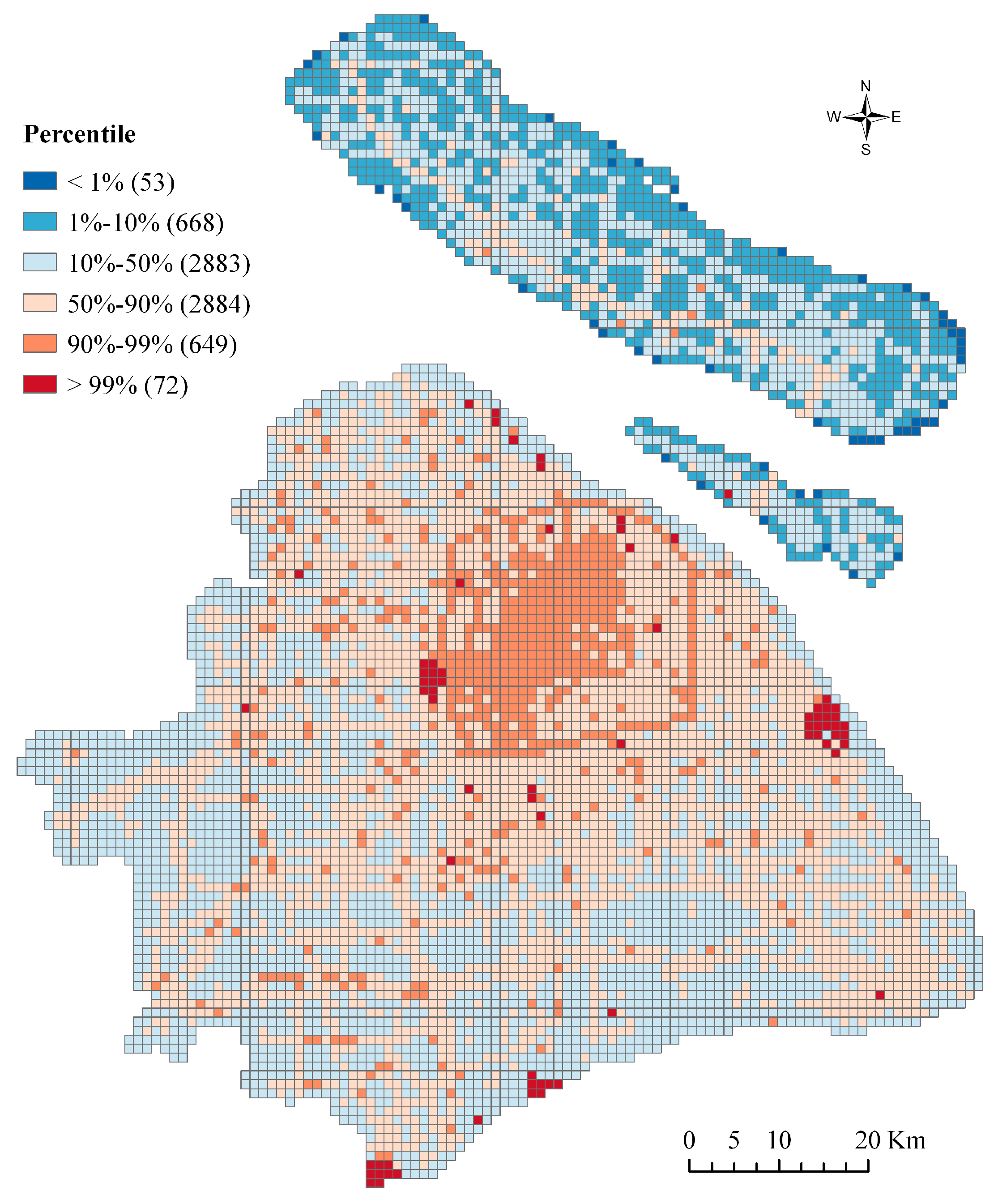
3.2.1. Spatial Differences in ffCO2 Emissions
3.2.2. The High Spatial Agglomeration of ffCO2 Emissions Has Not Changed over Time
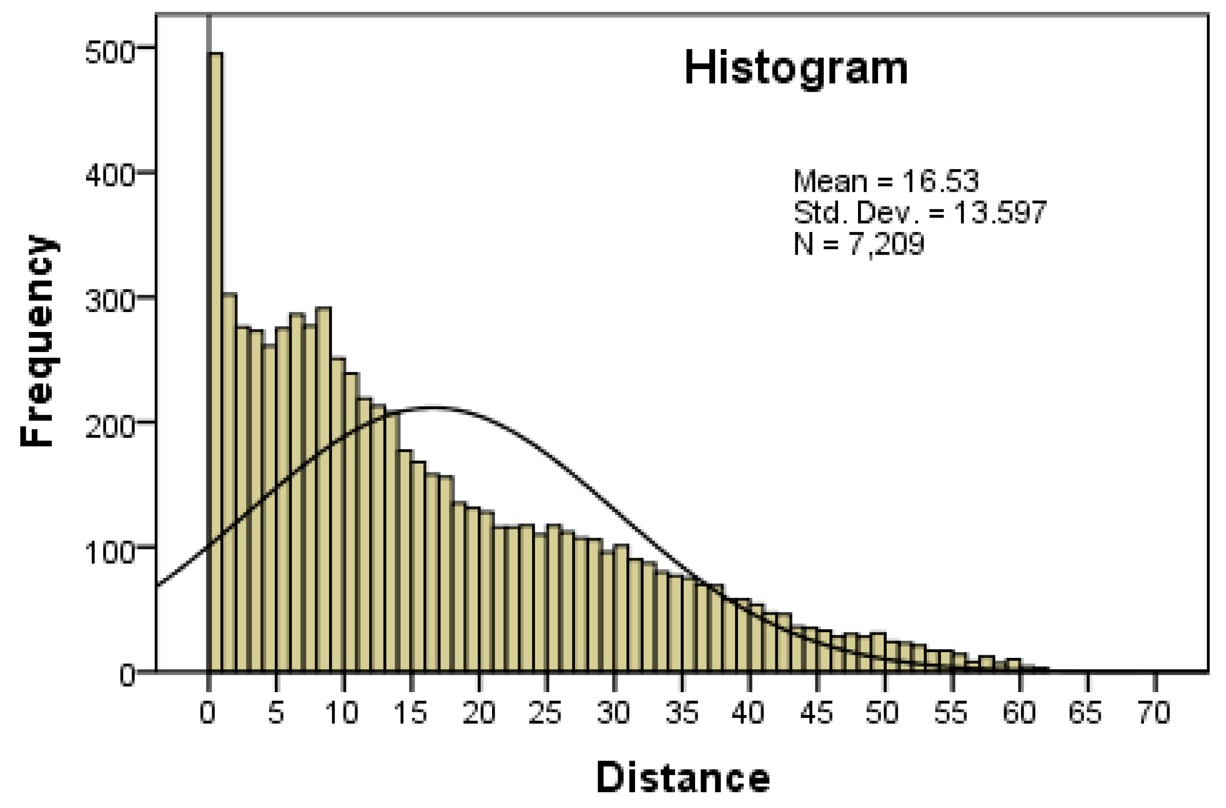
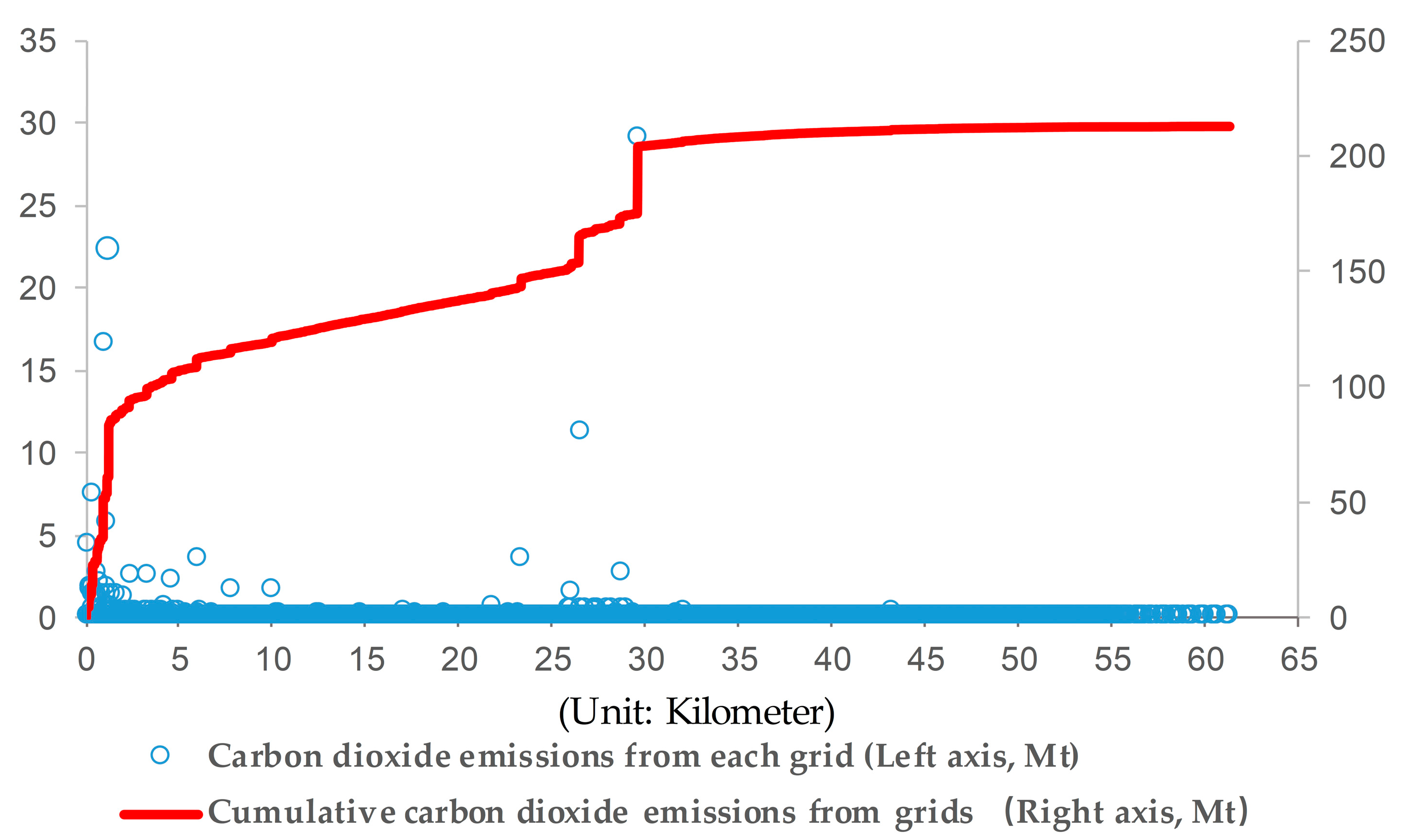
3.3. CO2 Emissions Concentrated along the River and Coastal Area
3.4. Circular Layers Structure of CO2 Emissions
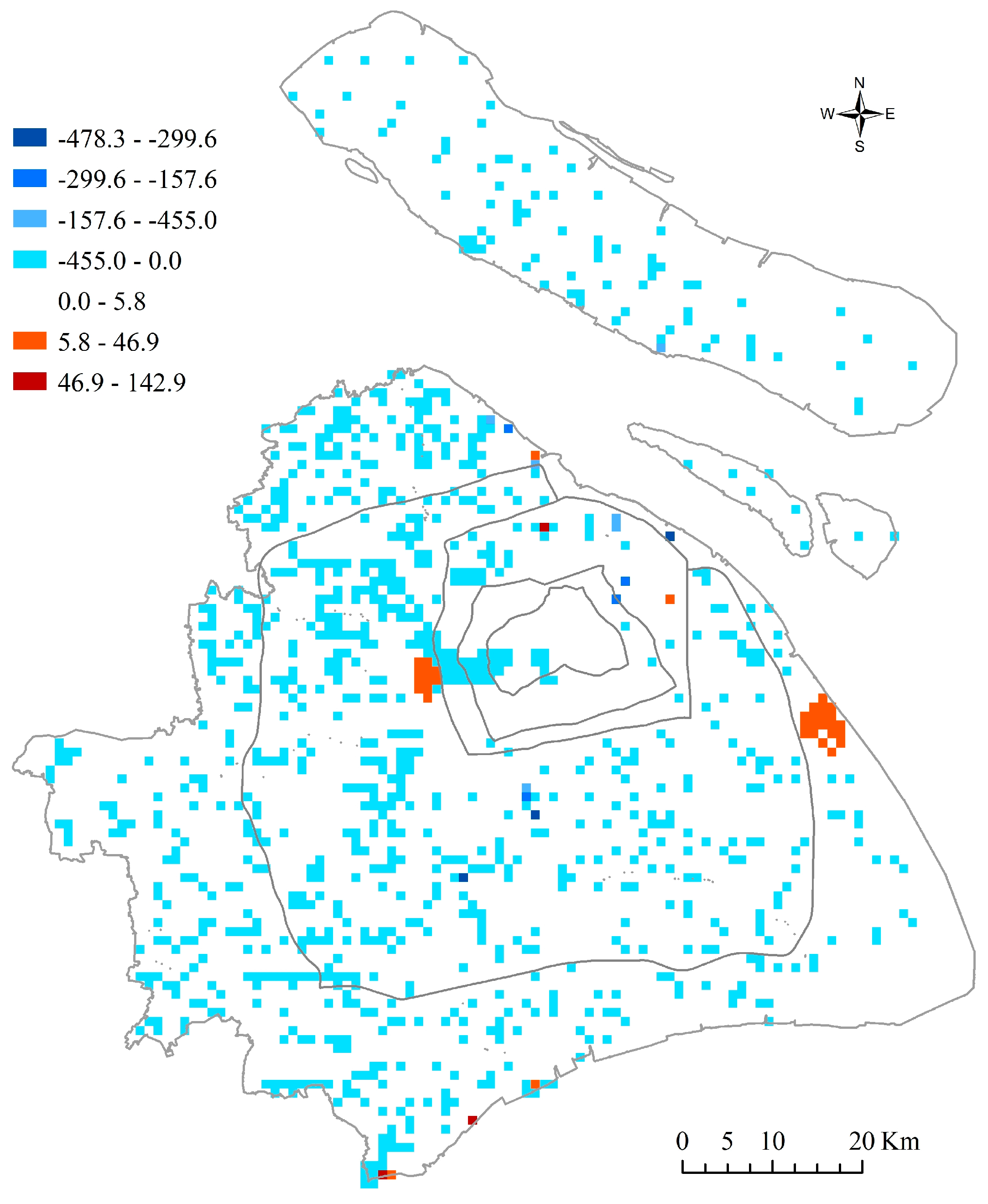
3.5. Differences in Grid Changes in CO2 Emissions
4. Impact Mechanisms of CO2 Emissions
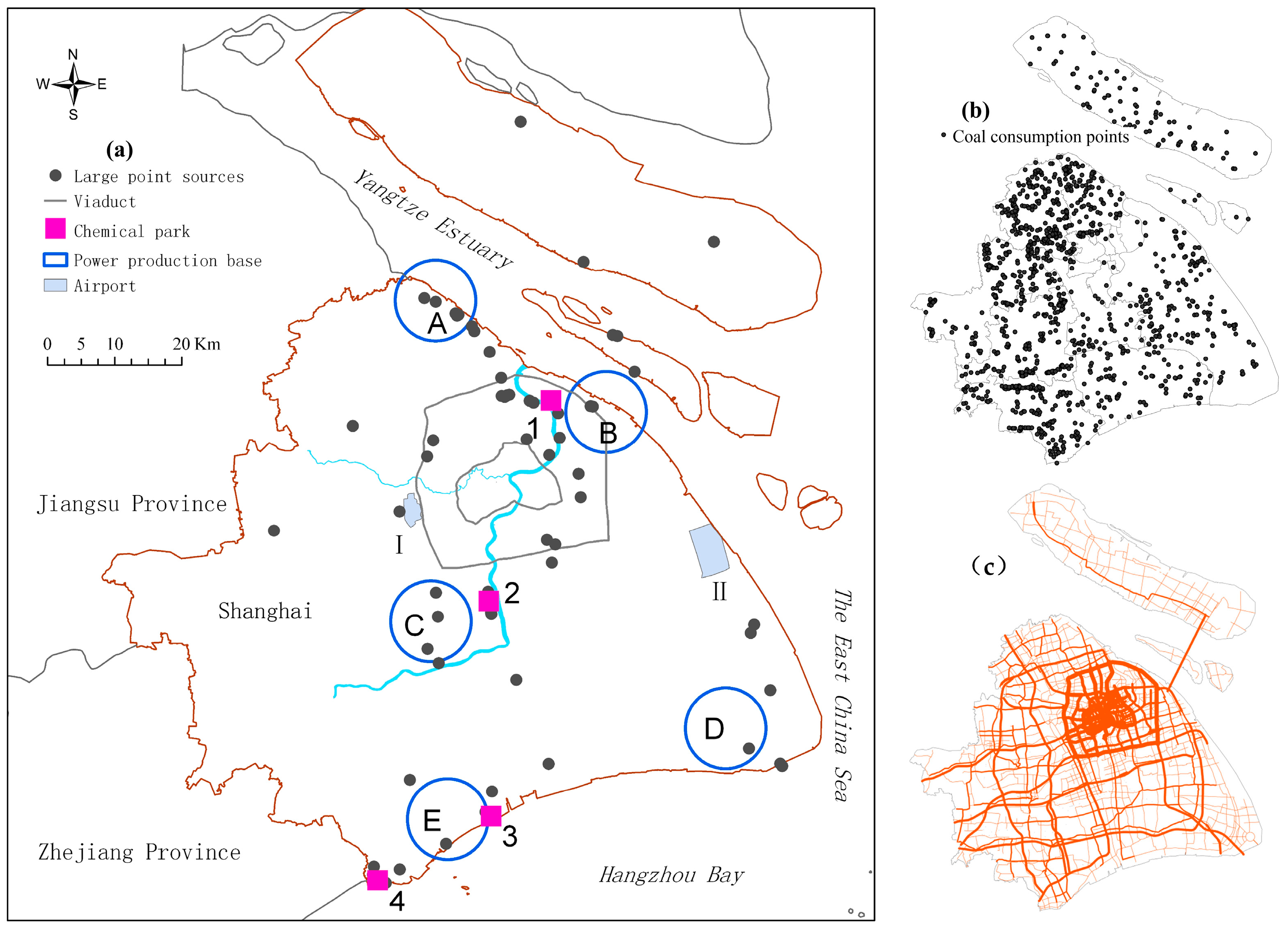
4.1. Impact Mechanisms of CO2 Emissions from Large Point Sources (LPS)
4.2. Impact Mechanisms of CO2 Emissions from Area Sources
5. Conclusions and Outlook
Supplementary Materials
Author Contributions
Funding
Acknowledgments
Conflicts of Interest
References
- Chen, L.; Frauenfeld, O.W. Impacts of urbanization on future climate in China. Clim. Dyn. 2016, 47, 345–357. [Google Scholar] [CrossRef]
- Seto, K.C.; Güneralp, B.; Hutyra, L.R. Global forecasts of urban expansion to 2030 and direct impacts on biodiversity and carbon pools. Proc. Natl. Acad. Sci. 2012, 109, 16083–16088. [Google Scholar] [CrossRef] [PubMed]
- Rosenzweig, C.; Solecki, W.; Hammer, S.A.; Mehrotra, S. Cities lead the way in climate–change action. Nature 2010, 467, 909–911. [Google Scholar] [CrossRef] [PubMed]
- Wang, S.H.; Huang, S.L.; Huang, P.J. Can spatial planning really mitigate carbon dioxide emissions in urban areas? A case study in Taipei, Taiwan. Landsc. Urban Plan. 2018, 169, 22–36. [Google Scholar] [CrossRef]
- Gurney, K.R.; Romero-Lankao, P.; Seto, K.C.; Hutyra, L.R.; Duren, R.; Kennedy, C.; Grimm, N.B.; Ehleringer, J.R.; Marcotullio, P.; Hughes, S.; et al. Climate change: Track urban emissions on a human scale. Nature 2015, 525, 179–181. [Google Scholar] [CrossRef] [PubMed]
- Patarasuk, R.; Gurney, K.R.; O’Keeffe, D.; Song, Y.; Huang, J.; Rao, P.; Buchert, M.; Lin, J.C.; Mendoza, D.; Ehleringer, J.R. Urban high-resolution fossil fuel CO2 emissions quantification and exploration of emission drivers for potential policy applications. Urban Ecosyst. 2016, 19, 1013–1039. [Google Scholar] [CrossRef]
- Liu, Z.; Geng, Y.; Xue, B. Inventorying energy-related CO2 for City: Shanghai study. Energy Procedia 2011, 5, 2303–2307. [Google Scholar] [CrossRef]
- Shan, Y.; Guan, D.; Liu, J.; Mi, Z.; Liu, Z.; Liu, J.; Schroeder, H.; Cai, B.; Chen, Y.; Shao, S.; et al. Methodology and applications of city level CO2 emission accounts in China. J. Clean. Prod. 2017, 161, 1215–1225. [Google Scholar] [CrossRef]
- Jing, Q.; Bai, H.; Luo, W.; Cai, B.; Xu, H. A top-bottom method for city-scale energy-related CO2 emissions estimation: A case study of 41 Chinese cities. J. Clean. Prod. 2018, 202, 444–455. [Google Scholar] [CrossRef]
- Gately, C.K.; Hutyra, L.R. Large uncertainties in urban-scale carbon emissions. J. Geophys. Res. Atmos. 2017, 122, 11,242–11,260. [Google Scholar] [CrossRef]
- Duren, R.M.; Miller, C.E. Measuring the carbon emissions of megacities. Nat. Clim. Chang. 2012, 2, 560–562. [Google Scholar] [CrossRef]
- Lei, L.P.; Guan, X.H.; Zeng, Z.C.; Zhang, B.; Ru, F.; Bu, R. A comparison of atmospheric CO2 concentration GOSAT-based observations and model simulations. Sci. China Earth Sci. 2014, 57, 1393–1402. [Google Scholar] [CrossRef]
- Breón, F.M.; Broquet, G.; Puygrenier, V.; Chevallier, F.; Xueref-Remy, I.; Ramonet, M.; Dieudonné, E.; Lopez, M.; Schmidt, M.; Perrussel, O.; et al. An attempt at estimating Paris area CO2 emissions from atmospheric concentration measurements. Atmos. Chem. Phys. 2015, 15, 1707–1724. [Google Scholar] [CrossRef]
- Pillai, D.; Buchwitz, M.; Gerbig, C.; Koch, T.; Reuter, M.; Bovensmann, H.; Marshall, J.; Burrows, J.P. Tracking city CO2 emissions from space using a high-resolution inverse modelling approach: A case study for Berlin, Germany. Atmos. Chem. Phys. 2016, 16, 9591–9610. [Google Scholar] [CrossRef]
- Newman, S.; Xu, X.; Gurney, K.R.; Hsu, Y.K.; Li, K.F.; Jiang, X.; Keeling, R.; Feng, S.; O’Keefe, D.; Patarasuk, R.; et al. Toward consistency between trends in bottom-up CO2 emissions and top-down atmospheric measurements in the Los Angeles megacity. Atmos. Chem. Phys. 2016, 16, 3843–3863. [Google Scholar] [CrossRef]
- Janardanan, R.; Maksyutov, S.; Oda, T.; Saito, M.; Kaiser, J.W.; Ganshin, A.; Stohl, A.; Matsunaga, T.; Yoshida, Y.; Yokota, T. Comparing GOSAT observations of localized CO2 enhancements by large emitters with inventory-based estimates. Geophys. Res. Lett. 2016, 43, 3486–3493. [Google Scholar] [CrossRef]
- Wang, Y.; Broquet, G.; Ciais, P.; Chevallier, F.; Vogel, F.; Kadygrov, N.; Wu, L.; Yin, Y.; Wang, R.; Tao, S. Estimation of observation errors for large-scale atmospheric inversion of CO2 emissions from fossil fuel combustion. Tellus Ser. B Chem. Phys. Meteorol. 2017, 69. [Google Scholar] [CrossRef]
- Konovalov, I.B.; Berezin, E.V.; Ciais, P.; Broquet, G.; Zhuravlev, R.V.; Janssens-Maenhout, G. Estimation of fossil-fuel CO2 emissions using satellite measurements of “proxy” species. Atmos. Chem. Phys. 2016, 16, 13509–13540. [Google Scholar] [CrossRef]
- Parshall, L.; Gurney, K.; Hammer, S.A.; Mendoza, D.; Zhou, Y.; Geethakumar, S. Modeling energy consumption and CO2 emissions at the urban scale: Methodological challenges and insights from the United States. Energy Policy 2010, 38, 4765–4782. [Google Scholar] [CrossRef]
- Gurney, K.R.; Mendoza, D.L.; Zhou, Y.; Fischer, M.L.; Miller, C.C.; Geethakumar, S.; Du Can, S.D.L.R. High resolution fossil fuel combustion CO2 emission fluxes for the United States. Environ. Sci. Technol. 2009, 43, 5535–5541. [Google Scholar] [CrossRef]
- Gurney, K.R.; Razlivanov, I.; Song, Y.; Zhou, Y.; Benes, B.; Abdul-Massih, M. Quantification of fossil fuel CO2 emissions on the building/street scale for a large U.S. City. Environ. Sci. Technol. 2012, 46, 12194–12202. [Google Scholar] [CrossRef] [PubMed]
- Feng, S.; Lauvaux, T.; Newman, S.; Rao, P.; Ahmadov, R.; Deng, A.; Díaz-Isaac, L.I.; Duren, R.M.; Fischer, M.L.; Gerbig, C.; et al. Los Angeles megacity: A high-resolution land-atmosphere modelling system for urban CO2 emissions. Atmos. Chem. Phys. 2016, 16, 9019–9045. [Google Scholar] [CrossRef]
- Oda, T.; Lauvaux, T.; Lu, D.; Rao, P.; Miles, N.L.; Richardson, S.J.; Gurney, K.R. On the impact of granularity of space-based urban CO2 emissions in urban atmospheric inversions: A case study for Indianapolis, IN. Elem Sci Anth 2017, 5, 28. [Google Scholar] [CrossRef]
- Wei, W.; Ren, X.; Cai, Z.; Hou, Q.; Liu, Y.; Li, Q. Research on China’s Greenhouse gas emission—Progress on emission inventory from the CAS strategic priority research program. Bull. Chin. Acad. Sci. 2015, 6, 839–848. (In Chinese) [Google Scholar]
- Wang, J.; Cai, B.; Zhang, L.; Cao, D.; Liu, L.; Zhou, Y.; Zhang, Z.; Xue, W. High resolution carbon dioxide emission gridded data for China derived from point sources. Environ. Sci. Technol. 2014, 48, 7085–7093. [Google Scholar] [CrossRef] [PubMed]
- Cai, B.; Wang, J.; Yang, S.; Mao, X.; Cao, L. Carbon dioxide emissions from cities in China based on high resolution emission gridded data. Chinese, J. Popul. Resour. Environ. 2017, 15, 58–70. [Google Scholar] [CrossRef]
- Pan, K.; Li, Y.; Zhu, H.; Dang, A. Spatial configuration of energy consumption and carbon emissions of Shanghai, and our policy suggestions. Sustainability 2017, 9, 104. [Google Scholar] [CrossRef]
- Penman, J.; Gytarsky, M.; Hiraishi, T.; Irving, W.; Krug, T. 2006 IPCC—Guidelines for National Greenhouse Gas Inventories; IPCC: Geneva, Switzerland, 2006. [Google Scholar]
- Pan, K.-X.; Zhu, H.-X.; Chang, Z.; Wu, K.-H.; Shan, Y.-L.; Liu, Z.-X. Estimation of coal-related CO2 emissions: The case of China. Energy Environ. 2014, 24, 1309–1321. [Google Scholar] [CrossRef]
- Wang, J.F.; Li, X.H.; Christakos, G.; Liao, Y.L.; Zhang, T.; Gu, X.; Zheng, X.Y. Geographical detectors-based health risk assessment and its application in the neural tube defects study of the Heshun Region, China. Int. J. Geogr. Inf. Sci. 2010, 24, 107–127. [Google Scholar] [CrossRef]
- Wang, J.F.; Hu, Y. Environmental health risk detection with GeogDetector. Environ. Model. Softw. 2012, 33, 114–115. [Google Scholar] [CrossRef]
- Wang, J.F.; Zhang, T.L.; Fu, B.J. A measure of spatial stratified heterogeneity. Ecol. Indic. 2016, 67, 250–256. [Google Scholar] [CrossRef]
- Lou, C.R.; Liu, H.Y.; Li, Y.F.; Li, Y.L. Socioeconomic drivers of PM2.5 in the accumulation phase of air pollution episodes in the Yangtze River Delta of China. Int. J. Environ. Res. Public Health 2016, 13, 928. [Google Scholar] [CrossRef] [PubMed]
- Bai, L.; Jiang, L.; Yang, D.-y.; Liu, Y.-b. Quantifying the spatial heterogeneity influences of natural and socioeconomic factors and their interactions on air pollution using the geographical detector method: A case study of the Yangtze River Economic Belt, China. J. Clean. Prod. 2019, 232, 692–704. [Google Scholar] [CrossRef]
- Tian, L.; Li, Y.; Yan, Y.; Wang, B. Measuring urban sprawl and exploring the role planning plays: A shanghai case study. Land use policy 2017, 67, 426–435. [Google Scholar] [CrossRef]
- Wu, R.; Zhang, J.; Bao, Y.; Zhang, F. Geographical detector model for influencing factors of industrial sector carbon dioxide emissions in Inner Mongolia, China. Sustainability 2016, 8, 149. [Google Scholar] [CrossRef]
- Kennedy, C.; Steinberger, J.; Gasson, B.; Hansen, Y.; Hillman, T.; Havránek, M.; Pataki, D.; Phdungsilp, A.; Ramaswami, A.; Mendez, G.V. Greenhouse gas emissions from global cities. Environ. Sci. Technol. 2009, 43, 7297–7302. [Google Scholar] [CrossRef] [PubMed]
- Marcotullio, P.J.; Sarzynski, A.; Albrecht, J.; Schulz, N.; Garcia, J. The geography of global urban greenhouse gas emissions: An exploratory analysis. Clim. Change 2013, 121, 621–634. [Google Scholar] [CrossRef]
- Wu, Y.; Shen, J.; Zhang, X.; Skitmore, M.; Lu, W. Reprint of: The impact of urbanization on carbon emissions in developing countries: a Chinese study based on the U-Kaya method. J. Clean. Prod. 2017, 163, S284–S298. [Google Scholar] [CrossRef]
- Seto, K.C.; Shepherd, J.M. Global urban land-use trends and climate impacts. Curr. Opin. Environ. Sustain. 2009, 1, 89–95. [Google Scholar] [CrossRef]
- Pan, H.; Zhang, L.; Cong, C.; Deal, B.; Wang, Y. A dynamic and spatially explicit modeling approach to identify the ecosystem service implications of complex urban systems interactions. Ecol. Indic. 2019, 102, 426–436. [Google Scholar] [CrossRef]
- Chuai, X.; Huang, X.; Wang, W.; Zhao, R.; Zhang, M.; Wu, C. Land use, total carbon emissions change and low carbon land management in Coastal Jiangsu, China. J. Clean. Prod. 2015, 103, 77–86. [Google Scholar] [CrossRef]
- Fu, B.; Wu, M.; Che, Y.; Yang, K. Effects of land-use changes on city-level net carbon emissions based on a coupled model. Carbon Manag. 2017, 8, 245–262. [Google Scholar] [CrossRef]
- Huang, Y.; Xia, B.; Yang, L. Relationship study on land use spatial distribution structure and energy-related carbon emission intensity in different land use types of guangdong, China, 1996–2008. Sci. World J. 2013, 2013, 309680. [Google Scholar] [CrossRef] [PubMed]
- Li, T.; Li, J.; Zhou, Z.; Wang, Y.; Yang, X.; Qin, K.; Liu, J. Taking climate, land use, and social economy into estimation of carbon budget in the Guanzhong-Tianshui Economic Region of China. Environ. Sci. Pollut. Res. 2017, 24, 10466–10480. [Google Scholar] [CrossRef] [PubMed]
- Liao, C.H.; Chang, C.L.; Su, C.Y.; Chiueh, P.T. Correlation between land-use change and greenhouse gas emissions in urban areas. Int. J. Environ. Sci. Technol. 2013, 10, 1275–1286. [Google Scholar] [CrossRef]
- Tian, L.; Shen, T. Evaluation of plan implementation in the transitional China: A case of Guangzhou city master plan. Cities 2011, 28, 11–27. [Google Scholar] [CrossRef]
- Ou, J.; Liu, X.; Li, X.; Chen, Y. Quantifying the relationship between urban forms and carbon emissions using panel data analysis. Landsc. Ecol. 2013, 28, 1889–1907. [Google Scholar] [CrossRef]
- Wang, S.; Liu, X.; Zhou, C.; Hu, J.; Ou, J. Examining the impacts of socioeconomic factors, urban form, and transportation networks on CO2 emissions in China’s megacities. Appl. Energy 2017, 185, 189–200. [Google Scholar] [CrossRef]
- Zhong, W.; Wang, D.; Xie, D.; Yan, L. Dynamic characteristics of Shanghai’s population distribution using cell phone signaling data (in Chinese). Geogr. Res. 2017, 36, 972–984. [Google Scholar]


| Top–Down Approach | Bottom–Up Approach | ||||||||
|---|---|---|---|---|---|---|---|---|---|
| Coal Total | Petroleum Products Total | Natural Gas | Coke Moving in from Other Provinces | Total ffCO2 | Coal Total | Petroleum Products Total | Natural Gas | Total ffCO2 | |
| 2010 | 130.7 | 96.3 | 9.1 | 2.6 | 238.7 | 130.5 | 72.7 | 9.3 | 212.6 |
| 2011 | 135.7 | 92.6 | 11.2 | 2.9 | 242.4 | 135.2 | 71.5 | 11.2 | 217.9 |
| 2012 | 126.4 | 96.0 | 13.0 | 1.5 | 236.8 | 126.4 | 75.1 | 12.8 | 214.3 |
| 2013 | 125.5 | 98.8 | 14.7 | 2.9 | 242.0 | 125.4 | 79.1 | 14.3 | 218.9 |
| 2014 | 108.7 | 96.7 | 14.6 | 4.9 | 224.9 | 108.7 | 77.7 | 14.2 | 200.7 |
| 2015 | 105.4 | 101.1 | 15.6 | 2.9 | 225.0 | 105.4 | 82.3 | 14.1 | 201.7 |
| Year | Units | Top 10 1 | Top 20 | Top 50 | Top 72 (1%) 2 | Top 100 | Top 702 | Other Grids 3 | Total Emissions |
|---|---|---|---|---|---|---|---|---|---|
| 2010 | Mt-CO2 | 105.9 | 126.5 | 151.5 | 159.3 | 163.5 | 184 | 24.9 | 208.9 |
| % | 50.69 | 60.56 | 72.52 | 76.26 | 78.27 | 88.08 | 11.92 | 100.0 | |
| 2011 | Mt-CO2 | 115.8 | 134.1 | 156.6 | 164.1 | 167.9 | 189.5 | 28.4 | 217.9 |
| % | 53.14 | 61.54 | 71.87 | 75.31 | 77.05 | 86.97 | 13.03 | 100.0 | |
| 2012 | Mt-CO2 | 112.5 | 129.1 | 149.6 | 156.8 | 160.4 | 182.8 | 31.5 | 214.3 |
| % | 52.50 | 60.24 | 69.81 | 73.17 | 74.85 | 85.30 | 14.70 | 100.0 | |
| 2013 | Mt-CO2 | 115 | 131.5 | 153.9 | 161.9 | 165.4 | 187.2 | 31.7 | 218.9 |
| % | 52.54 | 60.07 | 70.31 | 73.96 | 75.56 | 85.52 | 14.48 | 100.0 | |
| 2014 | Mt-CO2 | 98 | 113.9 | 135.3 | 143.3 | 146.7 | 168.4 | 32.3 | 200.7 |
| % | 48.83 | 56.75 | 67.41 | 71.40 | 73.09 | 83.91 | 16.09 | 100.0 | |
| 2015 | Mt-CO2 | 97.8 | 114.8 | 136.2 | 145 | 148.4 | 169.6 | 32.1 | 201.7 |
| % | 48.49 | 56.92 | 67.53 | 71.89 | 73.57 | 84.09 | 15.91 | 100.0 |
| Circle | Coal-Related CO2 | Oil-Related CO2 | Natural Gas-Related CO2 | Energy-Related CO2 |
|---|---|---|---|---|
| Pxii | 0.01 | 5.87 | 5.66 | 2.80 |
| Pdii | 0.00 | 1.01 | 0.62 | 0.45 |
| Pxio | 5.09 | 8.96 | 8.67 | 6.91 |
| Pdio | 2.27 | 7.99 | 5.77 | 4.85 |
| Aoo | 92.63 | 76.17 | 79.29 | 84.99 |
| Total | 100 | 100 | 100 | 100 |
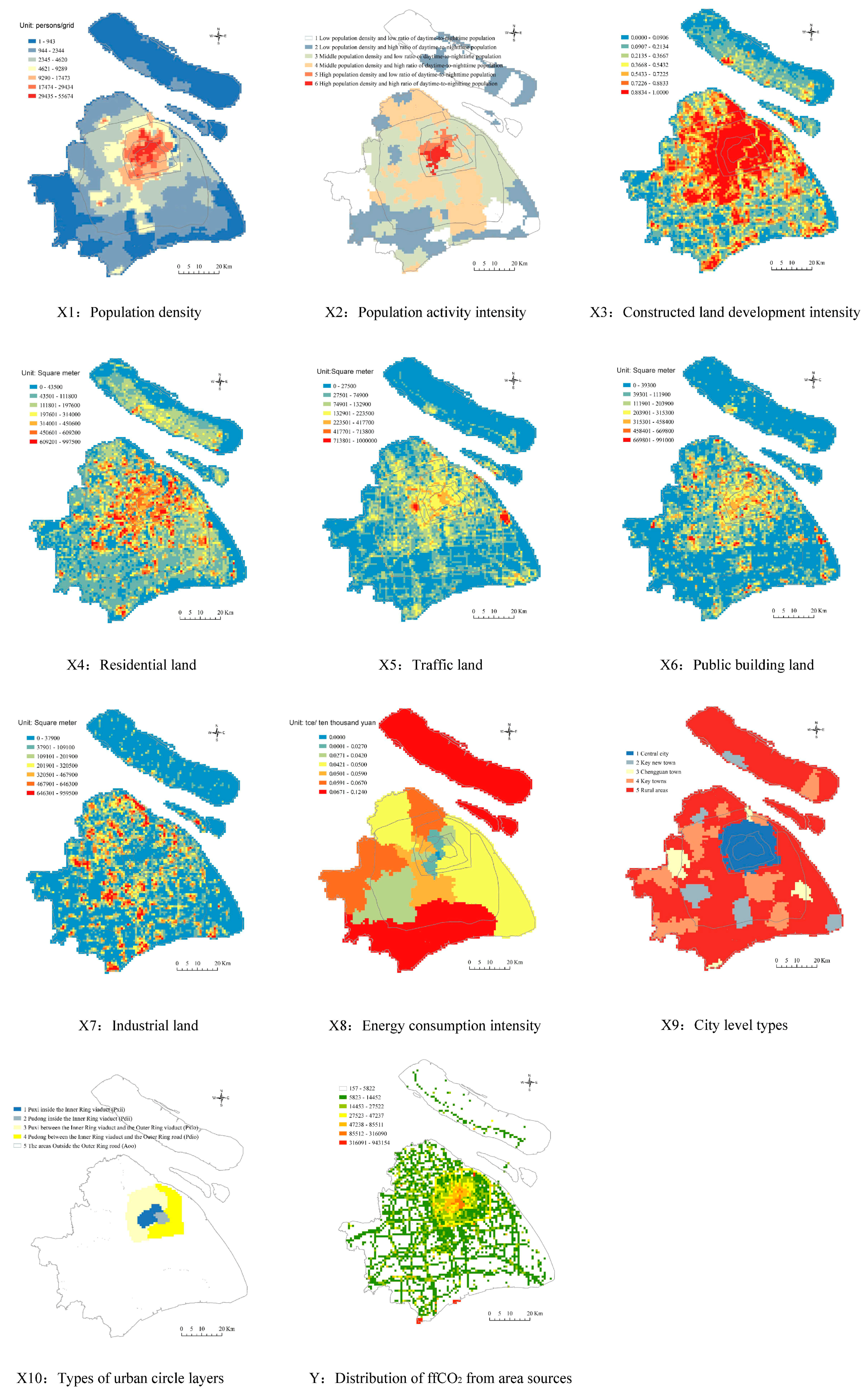
| Factor Types | Factors | Meaning | Data Resource |
|---|---|---|---|
| Population density | X1: Population density | Persons per grid (square kilometer) | Author mapped based on Shanghai Statistical Yearbook |
| Human activity intensity | X2: Population activity intensity | Street (township) is divided into six categories according to population density at the daytime and nighttime and the ratio of daytime-to-nighttime population. | Author mapped based on the study of [50] |
| X3: Constructed land development intensity | Constructed land area accounts for the proportion of the total area in each grid. | Author calculated | |
| Land-use types | X4: Residential land | The total area of residential land in each grid. | Author interpreted from high-resolution remote sensing image. |
| X5: Traffic land | The total area of traffic land in each grid. | ||
| X6: Public building land | The total area of public building land in each grid. | ||
| X7: Industrial land | The total area of industrial land in each grid. | ||
| Energy efficiency | X8: Energy consumption intensity | Energy consumption per 10000 RMB GDP output value of above-designated size enterprise. | Shanghai Statistical Yearbook on Energy |
| Urban planning | X9: City-level types | Including the central city, key new town, Chengguan town, key towns, and rural areas. | Shanghai Urban Plan (1999–2000) |
| X10: Types of urban circle layers | Including areas within the Inner Ring road, areas between Inner Ring road and Outer Ring road, and areas outside the Outer Ring road. | Shanghai Urban Plan (1999–2000) |
| Year | Value | X1 | X2 | X3 | X4 | X5 | X6 | X7 | X8 | X9 | X10 |
|---|---|---|---|---|---|---|---|---|---|---|---|
| 2010 | q statistic | 0.30 | 0.28 | 0.21 | 0.11 | 0.23 | 0.16 | 0.07 | 0.11 | 0.19 | 0.32 |
| p value | 0.00 | 0.00 | 0.00 | 0.00 | 0.00 | 0.00 | 0.00 | 0.00 | 0.00 | 0.00 | |
| 2015 | q statistic | 0.42 | 0.36 | 0.24 | 0.14 | 0.26 | 0.18 | 0.06 | 0.28 | 0.25 | 0.42 |
| p value | 0.00 | 0.00 | 0.00 | 0.00 | 0.00 | 0.00 | 0.00 | 0.00 | 0.00 | 0.00 |
| Circle | X1 | X2 | X3 | X4 | X5 | X6 | X7 | X8 | X9 | |
|---|---|---|---|---|---|---|---|---|---|---|
| Inner Ring | q statistic | 0.32 | 0.39 | 0.08 | 0.06 | 0.09 | 0.05 | 0.02 | 0.45 | -- |
| p value | 0.00 | 0.00 | 0.22 | 0.60 | 0.45 | 0.58 | 0.84 | 0.00 | -- | |
| Middle Ring | q statistic | 0.19 | 0.17 | 0.03 | 0.07 | 0.16 | 0.10 | 0.03 | 0.30 | 0.03 |
| p value | 0.00 | 0.00 | 0.07 | 0.00 | 0.00 | 0.00 | 0.03 | 0.00 | 0.04 | |
| Outer Ring | q statistic | 0.11 | 0.08 | 0.17 | 0.07 | 0.16 | 0.10 | 0.14 | 0.08 | 0.02 |
| p value | 0.00 | 0.00 | 0.00 | 0.00 | 0.00 | 0.00 | 0.00 | 0.00 | 0.00 |
© 2019 by the authors. Licensee MDPI, Basel, Switzerland. This article is an open access article distributed under the terms and conditions of the Creative Commons Attribution (CC BY) license (http://creativecommons.org/licenses/by/4.0/).
Share and Cite
Zhu, H.; Pan, K.; Liu, Y.; Chang, Z.; Jiang, P.; Li, Y. Analyzing Temporal and Spatial Characteristics and Determinant Factors of Energy-Related CO2 Emissions of Shanghai in China Using High-Resolution Gridded Data. Sustainability 2019, 11, 4766. https://doi.org/10.3390/su11174766
Zhu H, Pan K, Liu Y, Chang Z, Jiang P, Li Y. Analyzing Temporal and Spatial Characteristics and Determinant Factors of Energy-Related CO2 Emissions of Shanghai in China Using High-Resolution Gridded Data. Sustainability. 2019; 11(17):4766. https://doi.org/10.3390/su11174766
Chicago/Turabian StyleZhu, Hanxiong, Kexi Pan, Yong Liu, Zheng Chang, Ping Jiang, and Yongfu Li. 2019. "Analyzing Temporal and Spatial Characteristics and Determinant Factors of Energy-Related CO2 Emissions of Shanghai in China Using High-Resolution Gridded Data" Sustainability 11, no. 17: 4766. https://doi.org/10.3390/su11174766
APA StyleZhu, H., Pan, K., Liu, Y., Chang, Z., Jiang, P., & Li, Y. (2019). Analyzing Temporal and Spatial Characteristics and Determinant Factors of Energy-Related CO2 Emissions of Shanghai in China Using High-Resolution Gridded Data. Sustainability, 11(17), 4766. https://doi.org/10.3390/su11174766