Interpreting Daly’s Sustainability Criteria for Assessing the Sustainability of Marine Protected Areas: A System Dynamics Approach

Abstract

Sustainability assessments of marine protected areas (MPAs) are essential for improving the effectiveness of management efforts. Since sustainability is closely related to the concept of intergenerational well-being, measuring and tracking it through time is crucial. Therefore, this study will use the system dynamics approach applied at Pieh marine park as the study site. A system dynamics model was built comprising four sub-models: fish population dynamics, coral reef coverage, tourism, and pollution. The goodness-of-fit test of the model indicated low and unsystematic model error. The sustainability assessment was conducted using the three principles of sustainability proposed by Herman Daly, which define sustainability for resource management based on the change in the amount of renewable resources, non-renewable resources, and pollution. The sustainability assessment determined that Pieh marine park cannot sustain economic activities in its area, indicated by decreasing renewable resource indicators in the form of fish population dynamics, coral reef coverage, and increasing pollution levels. Several management interventions can be applied to improve sustainability, including lowering the total allowable catch, coral transplantation, and improved waste management.

1. Introduction

Marine and coastal ecosystems provide goods and services for human well-being, such as food provision, clean water, and tourism attractions. However, destructive fishing practices, overexploitation, environmental deterioration, land and water pollution, and global warming effects are leading to ecosystem degradation in coastal and marine areas [1]. Despite these dire impacts, the demand for fishery products around the globe is continually increasing each year [2], increasing pressure on marine and coastal environments.

One of the management tools to cope with various issues affecting marine and coastal environments is the implementation of marine protected areas (MPAs). An MPA is an area of intertidal or subtidal land with its surrounding waters and associated flora, fauna, historical, and cultural characteristics protected in part or whole by law or other effective means [3]. In particular, the primary goals of an MPA are to prevent the degradation of the coastal and marine environments, conserve biodiversity, avoid endangered species loss, sustain productivity, and, in particular, restore depleted fisheries [4]. With recent commitments made by governments around the globe, the creation of MPAs is planned to cover over 10% of the world’s seas by 2020. This target was agreed by the Member States of the United Nations as part of Sustainable Development Goal 14, for the conservation and sustainable use of the oceans, seas, and marine resources [5].

Although many countries support MPAs as a management strategy for conserving marine ecosystems and biodiversity, its sustainability remains unguaranteed with more than 90% of existing MPAs failing to achieve their management goals [6]. MPA evaluation studies are essential for improving the effectiveness of management efforts and optimizing the associated human and financial resource allocation results [7].

Several studies have been conducted to assess sustainability of MPAs. Arceo and Granados-Barba evaluated the sustainability of an MPA using a socio-economic approach incorporating productivity, stability and resilience, adaptability, equity, and self-management [8]. As this study emphasizes socio-economic aspects of MPAs, the ecological aspect which has a significant impact on the sustainability of MPAs was neglected. Moreover, Marques et al. conducted a study to identify several sustainability indicators of MPAs using the adaptive and participative approach which involves the major MPA stakeholders [9]. As this study uses the participatory approach, the result mainly described sustainability indicators from stakeholder perspectives, excluding economic factors which are also highly important for MPAs. An MPA serves as an instrument for both maintaining marine biodiversity and the functioning of the ecosystem, as well as improving socio-economic conditions by increasing revenues from fisheries production and tourism [7]. Therefore, sustainability assessment of an MPA should cover both conservation and economic activities.

Human activities affect the environment through the disturbance of energy and matter flow [10]. These changes in ecosystem processes influence biodiversity, change the ecological state of ecosystems, and impact both society and the economy. Marine tourism activities, such as diving and snorkeling, depend on the presence of coral reef ecosystems. This ecosystem also plays a vital role in the captive fishery as spawning, nursery, and feeding grounds for several commercial fish species. Therefore, keeping the coral reef healthy is essential, and should be the target for conservation activities. Furthermore, economic activities, such as tourism and fisheries, also negatively impact coral reefs. Mohamad et al. have found that tourism activities, such as scuba diving, snorkeling, fishing, and cruise trips, caused severe damage to coral reefs in the Sembilan islands, Malaysia [11]. They also noticed significant impacts of pollution and sedimentation on coral reefs. Moreover, fishery activities could initiate a shift in some reef communities from coral to algal dominated phases, and several fishing gears have a direct impact of habitat degradation of coral reefs [12]. It can be said that economic activities and coral reefs have complex cause and effect relationships. The challenge has been to understand the relationships between social/economic interests and associated environmental issues, which require practical evaluation techniques based on an interdisciplinary approach.

Sustainable development is often defined as development that satisfies current needs without risking the ability of future generations to satiate their own [13]. However, this definition is still a generalized concept, and is often criticized as being difficult to translate in operational terms. Therefore, Daly proposed three principles of sustainable resource management: (i) the withdrawal of resources cannot exceed the regeneration of resources; (ii) waste generation cannot exceed ecosystem ability to process waste; and (iii) in the long term, non-renewable resources cannot be utilized at all [14]. Since sustainability is closely related to the concept of intergenerational well-being, measuring and tracking it through time is crucial [15]. Therefore, this study will use the system dynamics approach, which enhances learning in complex and non-linear systems behavior over time, to assess the sustainability of an MPA [16].

This study will try to answer two questions. First, can the MPA sustain economic activities in its area? Although the MPA is a conservation tool to maintain biodiversity in marine and coastal ecosystems, it should also support the economic growth of coastal communities. These two objectives can be contradictory and a challenge for MPA sustainability. Second, how can the MPA be managed to assure its sustainability? To achieve these two objectives, MPA management should incorporate conservation and economic activities.

2. Materials and Methods

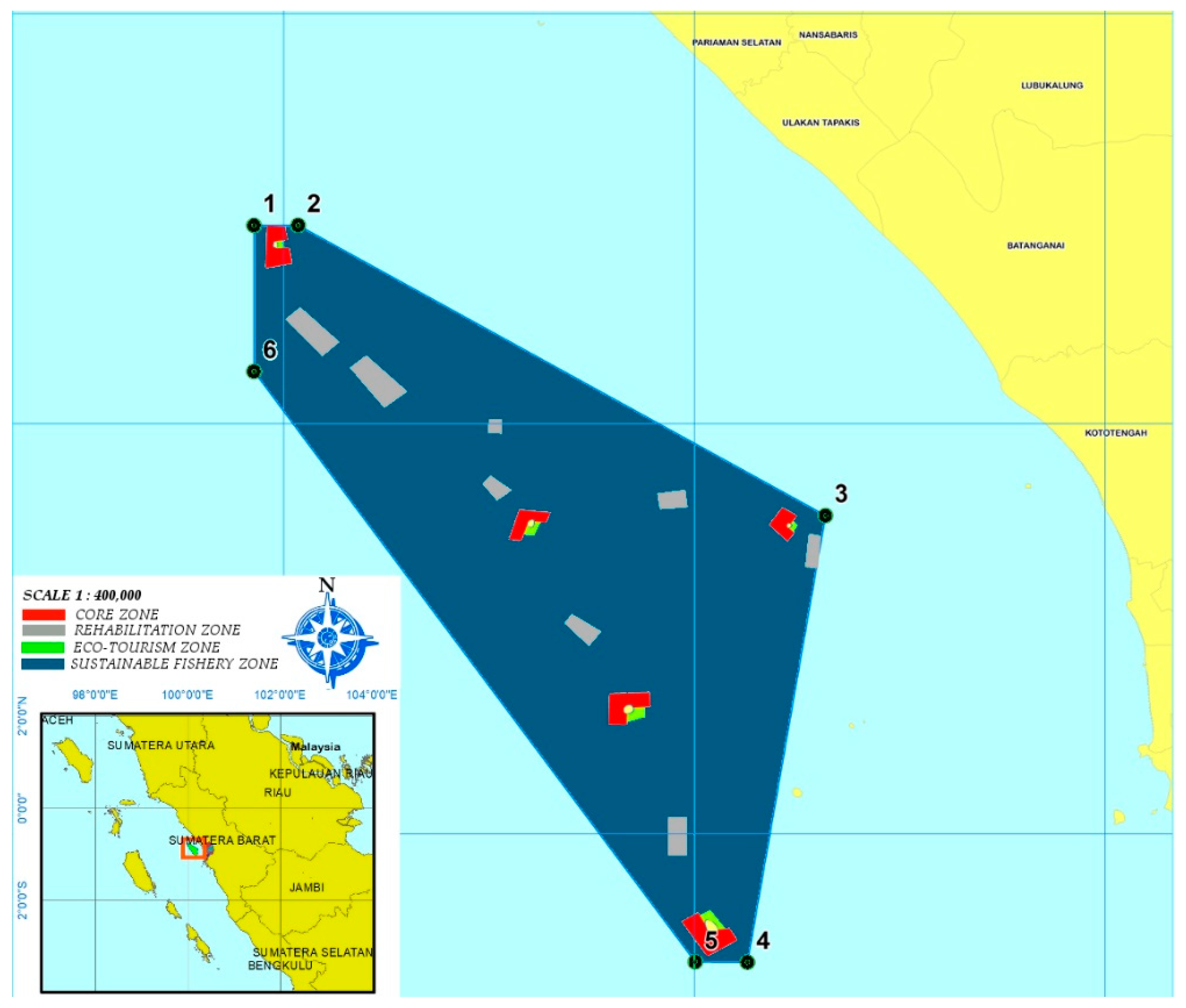
2.1. Study Site

This study was conducted at Pieh marine park, one of marine protected areas in Indonesia. This area, covering around 39,900 ha, was appointed as an MPA by Decree No. Kep.70/MEN/2009 from the Minister of Marine Affairs and Fisheries. This area includes the five small islands Pieh, Bando, Toran, Pandan, and Air Island. This marine park protects coral reefs and other species that occur there, such as coral fish, dolphins, and sea turtles. The Ministry of Marine Affairs and Fisheries have issued decree No. 38/KEPMEN-KP/2014 that divides Pieh marine park into four zones: the core zone (red), eco-tourism zone (green), rehabilitation zone (grey), and sustainable fishery zone (dark blue; Figure 1). The core zone, with a total area of around 801.59 ha, is strictly limited to fish habitat protection and research. However, the rehabilitation zone, which has a total area of around 1017.01 ha, functions as an area for coral reef rehabilitation. Pieh marine park supports tourism activities in the 106.68 ha eco-tourism zone. Fishery activities are designated to take place in the sustainable fishery zone, which covers around 37,974.72 ha.

The management goals of Pieh marine park are to protect and conserve natural resources in this area while still allowing economic activities, tourism, and fisheries, that abide by its zoning rules. Tourism in Pieh marine park can be categorized as mass tourism, with activities such as fishing, bathing, culinary activities, and mangrove or beach trekking. The number of visitors in the tourist destination in Padang Pariaman Regency showed an increasing trend from 2003 to 2007, but dropped in 2008 and then gradually increased again until 2017 (Figure 2a).

Pieh marine park also supports captive fishery activities at the Padang Pariaman Regency, which is categorized as a small-scale fishery whose primary target is demersal fish, such as flounders, tonguesoles, pomfrets, snappers, groupers, breams, and squids. The primary types of fishing gear used in this area are hooks, boat seines, and purse seines. Production in this sector showed an increasing trend from 2003 to 2005, but declined gradually from 2005 to 2017 (Figure 2b).

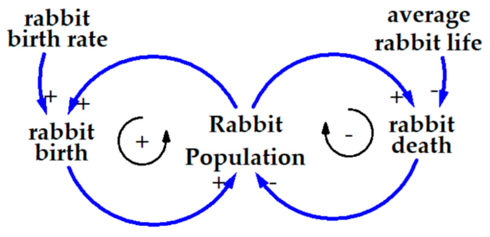
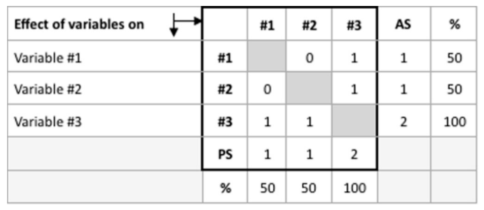
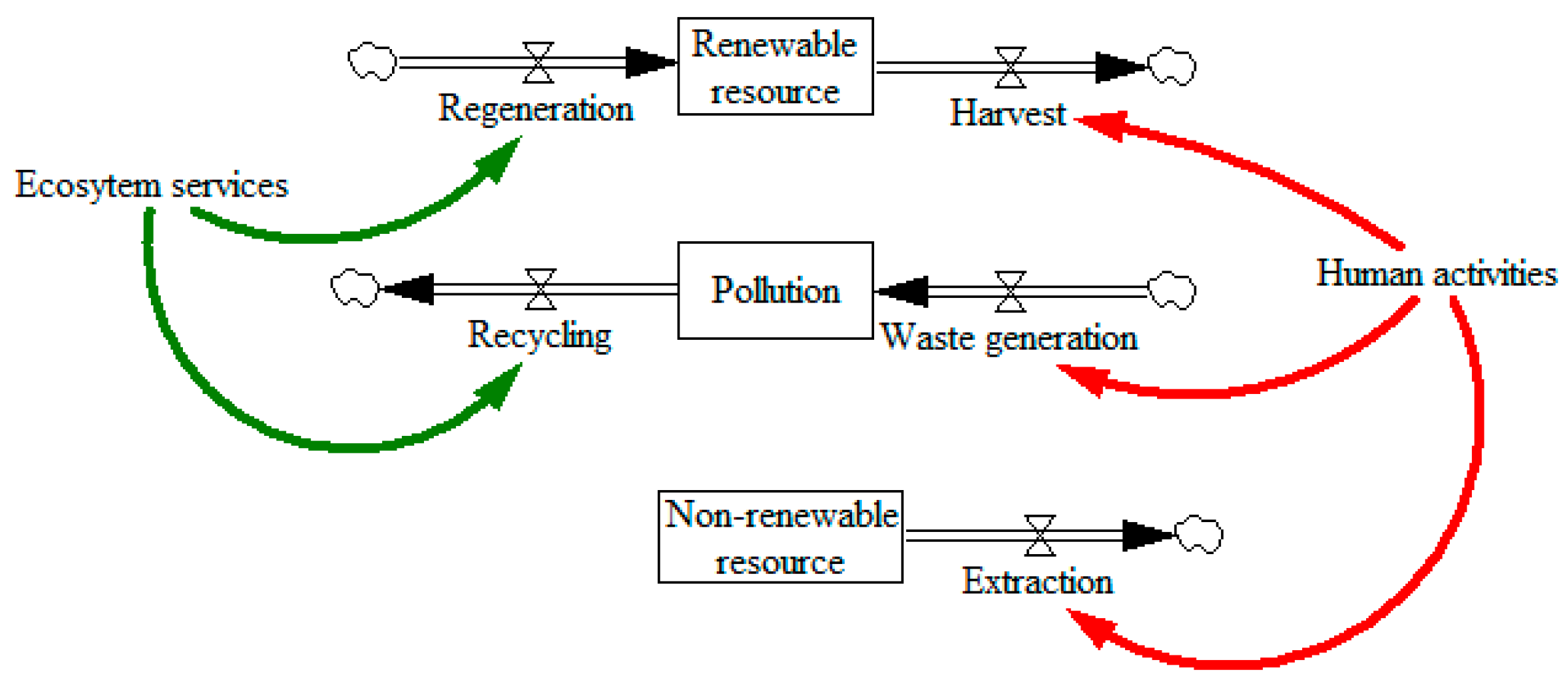
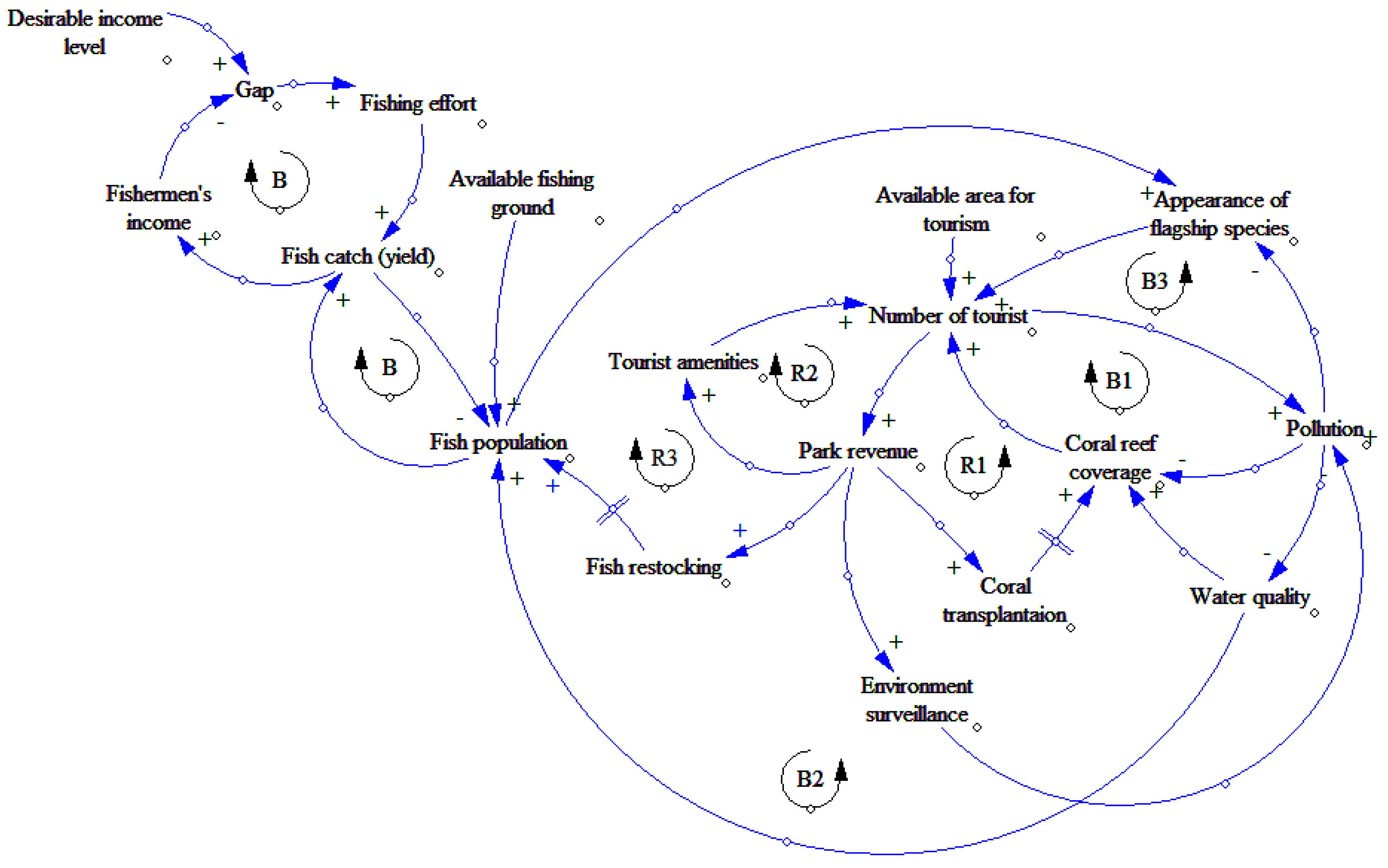
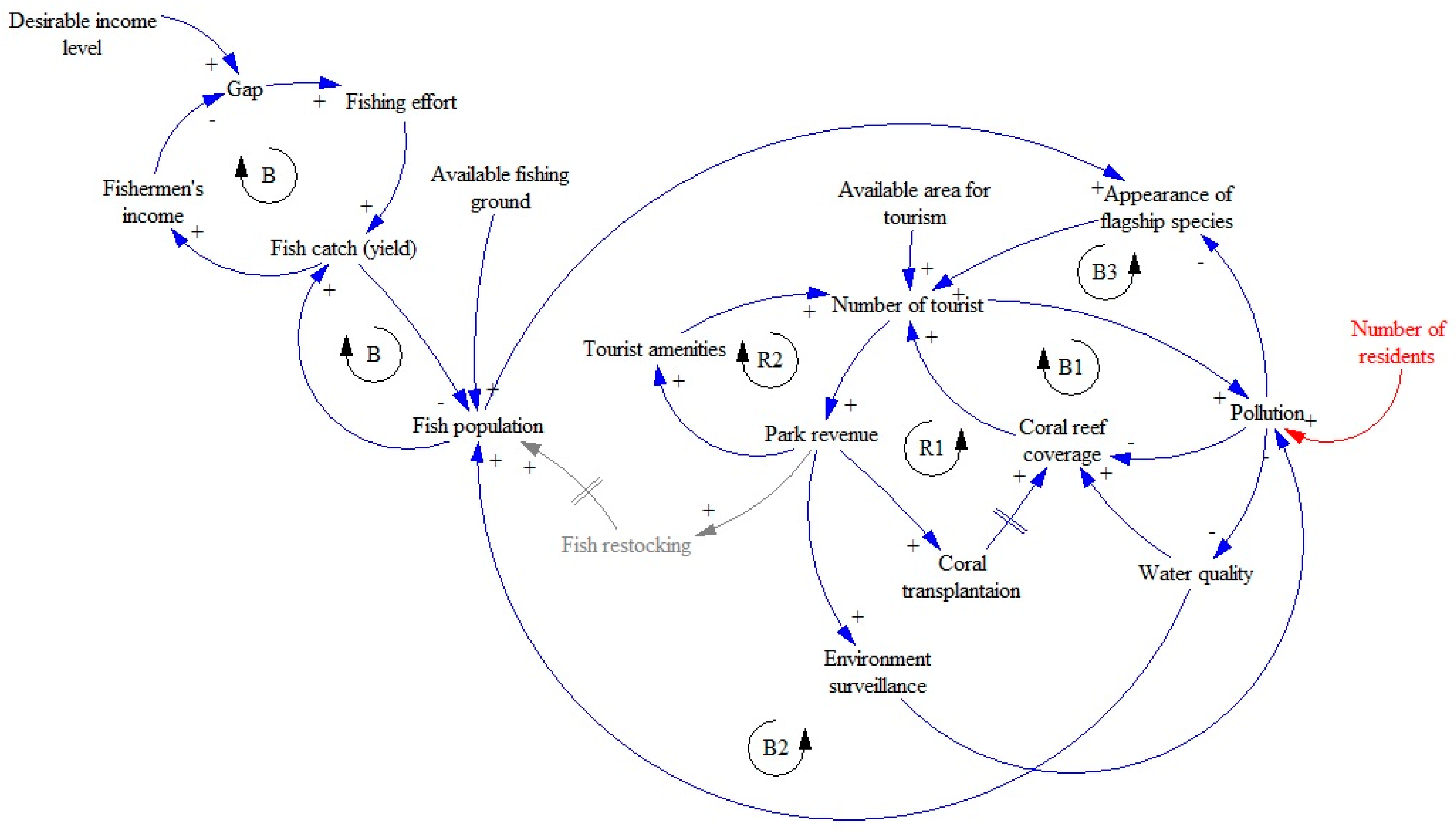
2.2. Causal Loop Diagram (CLD)

The causal loop was initially employed after simulation, to summarize and communicate model-based feedback insights, and also used before simulation analysis, to depict the underlying causal mechanisms hypothesized for the reference mode of behavior over time—that is, for the articulation of a dynamic hypothesis [17]. Causal Loop Diagrams (CLDs) are a particular type of model representation used in the system dynamics approach [16]. In this study, a CLD was built before the simulation analysis, as a qualitative description of the cause-effect relationships among conservation and economics activities in the study site, for capturing the dynamics of the marine park system.

CLDs are built through the identification of system variables that are linked to each other through arrows depicting cause-effect relationships. If variable ‘A’ is connected to variable ‘B’ through a positive link a ‘+’ sign is drawn to indicate that the variables change in the same direction, i.e., if ‘A’ increases, holding other conditions unchanged, ‘B’ increases. However, two variables connected by a negative ‘−’ sign, means that they change in opposite directions. Feedback loops are drawn when two or more variables are connected in a closed cycle. Feedback loops are classified as reinforcing (R) if they propagate an initial change in one of the loop variables, or balancing (B) if the loop counteracts the initial change. For example, a CLD of the rabbit population in Figure 3 shows that rabbit births and rabbit population create a reinforcing loop, while rabbit death and rabbit population create a balancing loop. Based on a CLD, the modeler may develop a dynamic hypothesis about the causal chain of effects that may happen if a particular change occurs within a system. Assumptions of the method consider that any cause-effect relationship depicted between two variables must be read ceteris paribus [18].

The CLD for Pieh marine park was constructed based on a literature review and then validated by stakeholders. Lopes and Videira have developed a method using a cross-impact matrix to determine which variables are relevant to a system [20]. This method involves valuing each variable’s response to other variables, where value “0” indicates that a given variable does not affect another, while value “1” indicates that a given variable does influence another. The values in rows (Active Sum/AS) and columns (Passive Sum/PS) are then summed up, with AS representing variables with more influence in the system and PS measuring how strongly a variable is affected by other variables. Variables with a high AS value can be translated into indicators of management points in the system, while variables with a high PS value can be translated into indicators of system changes. An example of cross-impact matrix calculation is shown in Figure 4. This analysis is a valuable complement to the interpretation of CLDs because all the identified variables result from a coherent analysis of the observed causal links [20]. Variables that have a high AS/PS ratio (more than 50%) would be the key variables in the system dynamics model.

2.3. System Dynamics Modelling

System dynamics (SD) is a technique used to describe, model, simulate, and analyze the process, information, organizational boundaries, and strategies of dynamically complex issues and systems [19]. A system is regarded as dynamic when its current output is based on previous inputs. If this is not the case, the system is regarded as static. In SD models, diagrammatic distinctions are made between different types of variables (stocks, flows, auxiliaries, parameters, and constants). Stocks are integral equations of the flows, flows and auxiliaries are equations of other variables and parameters/constants, and parameters/constants assume (constant) values over a simulation run. Links between variables and parameters in SD models represent only direct causal relationships. Hence, direct causal relationships need to be perceived, identified, or assumed for SD to be of any use. Under these conditions, SD can be used to explore the interaction between the (assumed) structure and the dynamically complex behavior of the issues. This can, for example, inform the transformation of structures to steer the system towards more desirable behaviors.

System dynamics modeling is based on a continuous feedback mechanism, incorporating the hypothesis of causal parameters and variable connections as a functional form [21]. Although there are different conventions in naming and the activities covered by each stage, the SD modeling process can be summarized as follows:

• Problem identification: identify and articulate the problem to be dealt with;
• Model conceptualization: develop a causal theory about the problem;
• Model formulation: formulate an SD simulation model of the causal theory;
• Model testing: test the model to assess whether it is fit for the purpose; and
• Model use, quite often model-based policy analysis: use the model to design and evaluate structural policies to address the problem.

Model testing comprises a wide variety of tests examining model structure, historical data fit, and model behavior [16], for example. The model structure was verified by a literature study and discussions with stakeholders. The model’s goodness of fit compared to historical data, is measured by mean-square-error (MSE), which defined as:

$$MSE=\frac{1}{n}{{\displaystyle \sum }}_{t=1}^n{\left(S_t-A_t\right)}^2.$$

(1)

• n = number of observation (t = 1, 2, …, n);
• S_t = simulated value at t;
• A_t = actual value at t.

However, it is often more convenient to compute a normalized measure of error. A common and easily interpreted dimensionless quantity is the root-mean-square-percentage-error (RMSPE), which ranges from 0 to 1, and is defined as:

$$RMSPE=\sqrt{\frac{1}{n}{\displaystyle \sum }_{t=1}^n{\left(\frac{S_t-A_t}{A_t}\right)}^2}.$$

(2)

In addition to the size of the total error, it is crucial to know the source of error. Failure to fit the historical data may be caused by a poor model or by a significant degree of randomness in the historical data. The Theil’s inequality statistics provide one elegant decomposition of the MSE. The Theil’s statistics are derived from the following decomposition of MSE:

$$\begin{array}{c}MSE={\left(\overline{S}-\overline{A}\right)}^2+{\left(s_S-s_A\right)}^2+2\left(1-r\right)s_S{s}_A\\ U^M=\frac{{\left(\overline{S}-\overline{A}\right)}^2}{MSE};U^S=\frac{{\left(s_S-s_A\right)}^2}{MSE}; U^C=\frac{2\left(1-r\right)s_S{s}_A}{MSE}.\end{array}$$

(3)

• $\overline{S}$ and $\overline{A}$ = the mean of simulated and actual value;
  s_S and s_A = the standard deviation of simulated and actual value;
• $r=\frac{\raisebox{1ex}{$1$}\!\left/ \!\raisebox{-1ex}{$n$}\right.{\displaystyle \sum }\left(S_t-\overline{S}\right)\left(A_t-\overline{A}\right)}{s_S{s}_A}$ (correlation coefficient between simulated and actual value).
• U^M, U^S, and U^C = the fraction of MSE due to bias, unequal variance, and unequal covariance, respectively.

Each term is considered in turn to see how the inequality statistics apply. Bias can be thought of as a translation of one series by a constant amount at all points in time. A significant value of U^M reveals a systematic difference between the model and reality. Error due to bias is potentially severe, possibly indicating a specification or parameter error. Alternatively, bias may be due to acceptable simplifying assumptions which do not compromise the model. Error due to unequal variance indicates a cyclic mode in one series that is not present in the other. The interpretation of such situations depends on the purpose of the model. If the model is designed to investigate the cyclic mode, a substantial value of U^S would be a systematic error. However, if the purpose of the model is an analysis of long-term behavior extrapolated from a short-term cycle, a substantial value of U^S becomes an unsystematic error. If the majority of error is concentrated in U^C, it indicates that the point-by-point values of the simulated and actual series do not match, even though the model captures the average value and dominant trends in the actual data well. A significant value of U^C indicates that the majority of error is unsystematic. A good model should have a small error, with RMSPE value close to 0, and the error should be unsystematic, which is concentrated in U^S or U^C.

Model behavior is investigated using a sensitivity analysis by changing the values of several parameters simultaneously using a uniform distribution within a specified range. The system dynamics modeling and sensitivity analysis were conducted using the software Vensim.

2.4. Sustainability Assessment

Sustainability is a generalized concept, and is often criticized as being difficult to translate in operational terms. It does not have defined parameters that can be scientifically defined. Therefore, Daly proposed three simple rules to help define the sustainable limits to material and energy throughput: (i) for renewable resources, the sustainable rate of use cannot be higher than the rate of regeneration; (ii) for non-renewable resources, the sustainable rate of use cannot be higher than the rate a renewable resource can be substituted; and (iii) for pollutants, the sustainable rate of emissions cannot be higher than the rate at which that pollutant can be recycled, absorbed, or rendered harmless in its sink [14].

Those three conditions of sustainability can be written using a stock and flow diagram, as in Figure 5. Rectangles denote stocks, while pipes and valves denote the flows. Here, the stock of renewable resources is depleted by harvesting (e.g., fishing) and renewed by regeneration (e.g., fish reproduction). The harvest of renewables, generation of waste, and extraction of non-renewables are driven by human activity (the population and economy). Renewable resource regeneration and the processes that render waste harmless (e.g., breakdown of sewage, removal of CO2 from the atmosphere) are provided by ecosystem services [22].

3. Results

3.1. Causal Loop Diagram

As the main economic activities in Pieh marine park are captive fishery and tourism related, several studies on these activities were used to create a hypothetical CLD using a system dynamics approach. Dudley developed a fishery model that examine complex fisheries issues in a transparent and comprehensible way without relying too heavily on population dynamics [23]. His model is based on the dynamic biomass model, which calculates the rate of fish population change based on fish growth, fishing catch, and fishing effort. For the relationship between coral reef and tourism, Chang et al. developed a coral reef management model involving tourist activities and environmental pressures [24]. Similarly, Tan et al. created an integrated coastal zone management model that includes tourist activities and pollution [25]. From these studies, a hypothetical CLD consisting of the fishery, coral reef, tourism, and pollution was proposed (Figure 6).

This CLD was discussed with Pieh marine park management officers to verify whether the relationship among variables is correct. The officers reported that pollution in Pieh marine park not only comes from tourists but also from residents who live along the coast. They also agreed to the removal of the ‘fish restocking’ variable because their management plan does not include fish restocking activities. The verified CLD can be seen in Figure 7.

The CLD makes several essential loops clear. First, the coral rehabilitation loop that starts with a good quality coral reef will attract more tourists, which will produce more revenue that can subsequently be invested in coral transplantation activities to improve the condition of the coral reef even further. However, more tourists also result in more pollution, leading to a declining water quality that affects the coral reef decay rate. This process creates a balancing loop for the effect of tourism on the coral reef. The next loop for tourism development starts with the development of tourist amenities that attract more tourists and revenue, which can then be invested in developing further tourist amenities. The last loop for the effect of tourism on the fish population starts from the fish population, which supports flagship species such as dolphins and sea turtles. Their presence attracts tourists, who produce more pollution, resulting in a decline in water quality. This reduced water quality impairs the regeneration rate of fish populations.

The cross-impact matrix method was implemented to determine which variables are relevant to the system (

Table 1. Cross-impact matrix of the CLD for Pieh marine park.

Variables	a	b	c	d	e	f	g	h	i	j	k	l	m	n	o	p	AS	%
a. Fish population		0	1	0	0	0	0	0	1	0	0	0	0	0	0	0	2	67
b. Available fishing ground	1		0	0	0	0	0	0	0	0	0	0	0	0	0	0	1	33
c. Fish catch	1	0		1	0	0	0	0	0	0	0	0	0	0	0	0	2	67
d. Fishermen’s income	0	0	0		1	0	0	0	0	0	0	0	0	0	0	0	1	33
e. Fishing effort	0	0	1	0		0	0	0	0	0	0	0	0	0	0	0	1	33
f. Coral reef coverage	0	0	0	0	0		0	1	0	0	0	0	0	0	0	0	1	33
g. Water quality	1	0	0	0	0	1		0	0	0	0	0	0	0	0	0	2	67
h. Number of tourists	0	0	0	0	0	0	0		0	1	0	0	1	0	0	0	2	67
i. Appearance of flagship species	0	0	0	0	0	0	0	1		0	0	0	0	0	0	0	1	33
j. Pollution	0	0	0	0	0	1	1	0	1		0	0	0	0	0	0	3	100
k. Available area for tourism	0	0	0	0	0	0	0	1	0	0		0	0	0	0	0	1	33
l. Tourist amenities	0	0	0	0	0	0	0	1	0	0	0		0	0	0	0	1	33
m. Park revenue	0	0	0	0	0	0	0	0	0	0	0	1		1	1	0	3	100
n. Coral transplantation	0	0	0	0	0	1	0	0	0	0	0	0	0		0	0	1	33
o. Environment surveillance	0	0	0	0	0	0	0	0	0	1	0	0	0	0		0	1	33
p. Number of residents	0	0	0	0	0	0	0	0	0	1	0	0	0	0	0		1	33
PS	3	0	2	1	1	3	1	4	2	3	0	1	1	1	1	0
%	75	0	50	25	25	75	25	100	50	75	0	25	25	25	25	0

). Fish population, fishing catch, water quality, number of tourists, pollution, and park revenue all have a large AS value (>50%). These variables are therefore suitable for monitoring management actions due to their substantial impact on the system. Fish population, coral reef coverage, number of tourists, and pollution also have a high PS value (>50%), therefore representing good options as indicators for monitoring change in the system. Interestingly, the fish population, number of tourists, and pollution have a high value for both the active and passive sum and can therefore be considered key stocks in the system, while coral reef coverage is the indicator of system change.

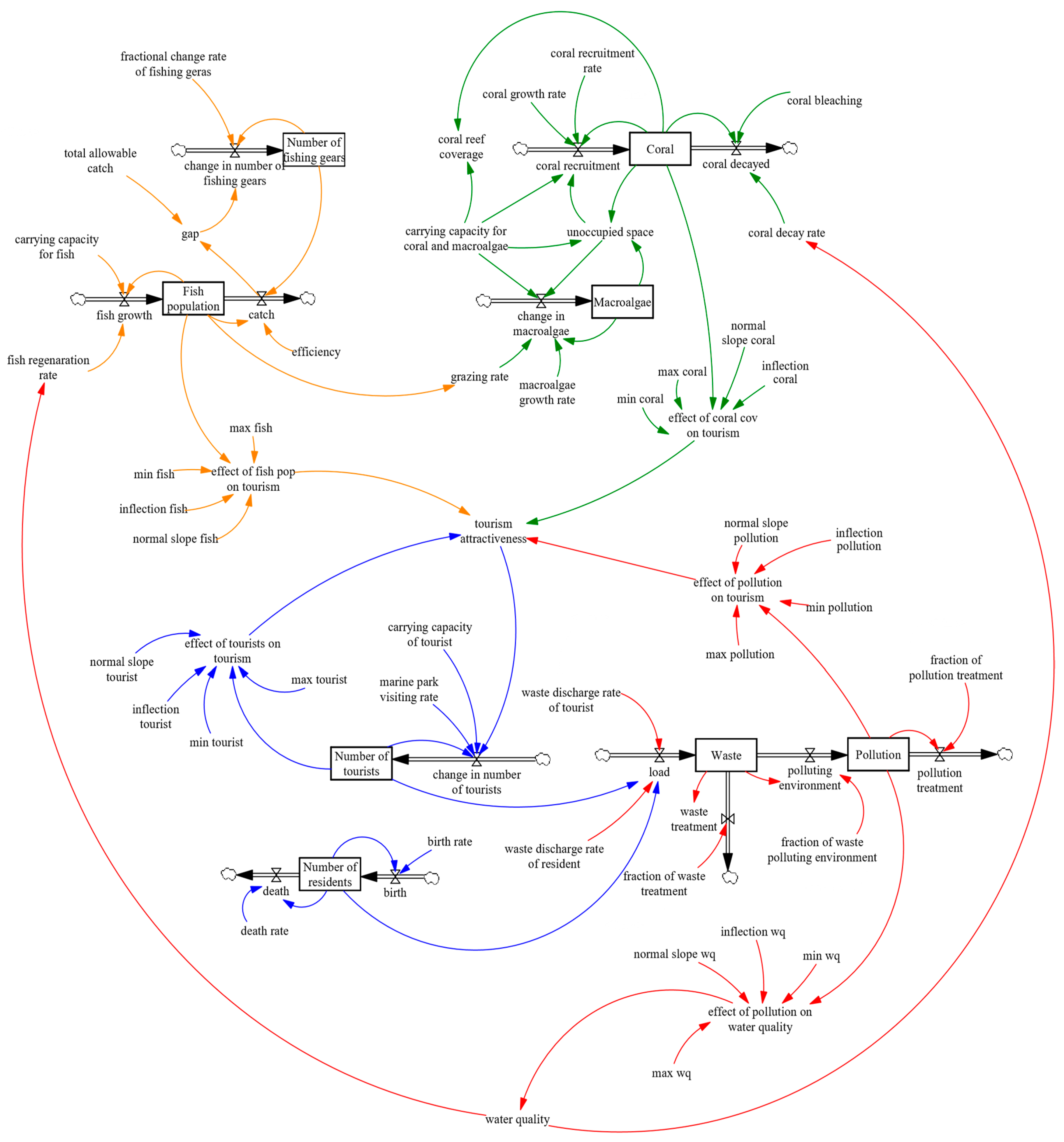
3.2. System Dynamics Modelling

A stack and flow diagram of the system dynamics model of this study can be seen in Figure 8. This model consists of the following four sub-models; fish population dynamics, coral reef coverage dynamics, tourism dynamics, and pollution dynamics. Fish population dynamics is connected to coral reef coverage dynamics by grazing activity of fish for macroalgae, which is the competitor of coral reef. Furthermore, both fish population and coral reef dynamics are connected to tourism dynamics as the main tourist attraction. Tourism dynamics is subsequently connected to pollution dynamics as the source of waste loading. Lastly, pollution dynamics alters the water quality that modifies fish population regeneration rate and coral decay rate, reducing tourism attractiveness. Details of the model is presented in Appendix A.

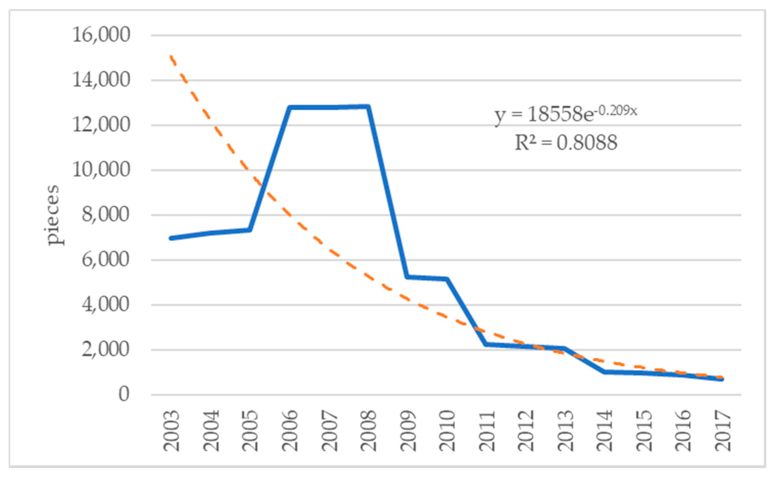
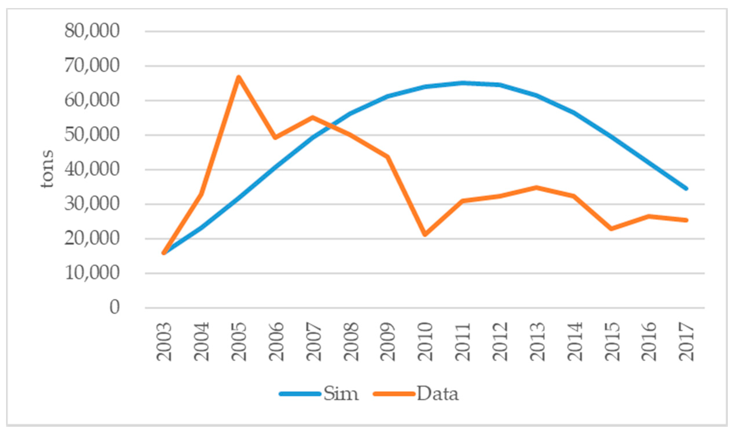
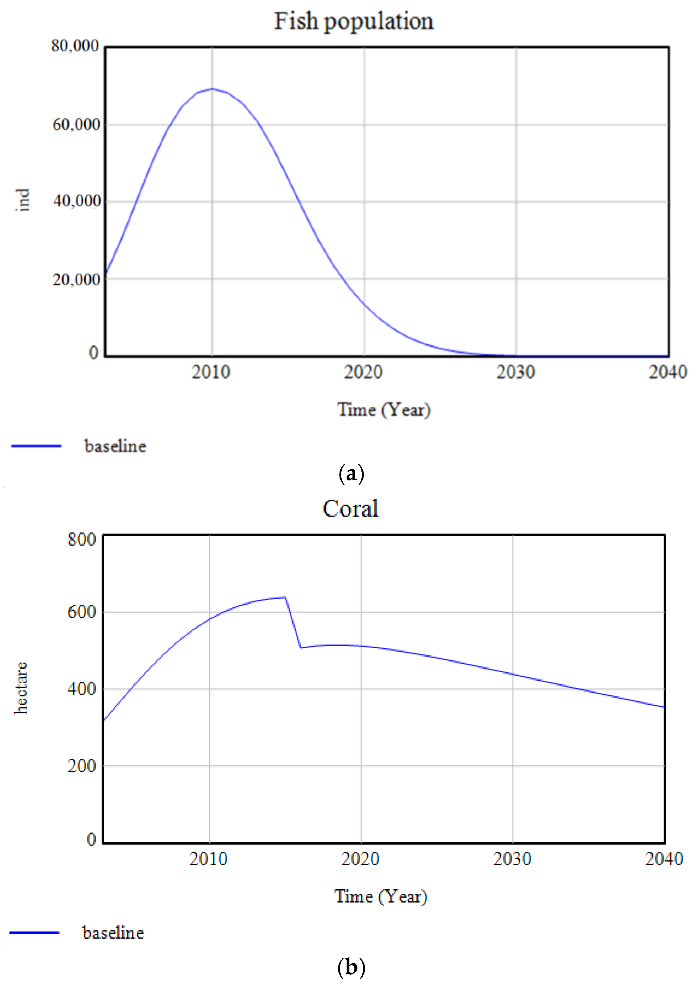
3.2.1. Fish Population Dynamics

The fish population model is based on the dynamic biomass (Gordon–Schaefer) model, which states that the increase in fish population due to reproduction is equal to the fish growth rate multiplied by the existing population, minus the natural decrease in fish multiplied by the ratio of fish population to the fish stock carrying capacity. The outflow of fish stock, a result of the catch, is indicated by the instantaneous fraction of fish biomass caught by each effort multiplied by the fishing effort, multiplied by the fish population [23]. From a system dynamics point of view, this process is best written as:

$$\frac{dB}{dt}=rB\left(1-\frac{B}{K}\right)-qXB.$$

(4)

• B = fish population;
• r = fish growth rate;
• K = fish stock carrying capacity;
• X = fishing effort;
• q = fraction of fish biomass caught by each effort.

To estimate the value of r, q, and K, this equation is transformed into linear equation as follow:

B_t+1 = B_t + rB_t (1 − B_t/K) − qX_tB_t.

(5)

By multiplying both sides with q, the equation becomes:

qB_t+1 = qB_t + rqB_t (1 − B_t/K) − q²X_tB_t
     = qB_t + rqB_t − rqB_t²/K − q²B_tX_t
     = (1 + r) qB_t − rq²B_t²/qK − q²B_tX_t
        = (1 + r) qB_t − (r/qK) (qB_t)² – qX_t (qB_t).

Since catch is qXB, catch per unit effort (CPUE) is qB. Therefore, the equation can be written:

CPUE_t+1 = (1 + r) CPUE_t − (r/qK) CPUE_t² − (q) X_tCPUE_t.

(6)

The variables that can be used as a proxy of fishing effort are the number of fishermen, fishing vessels, and fishing gears. CPUE equation can be used to find the best variable as a proxy of fishing effort and to find the values of r, q, and K by using multiple linear regression with the data provided in

Table 2. Data input for multiple linear regression of catch per unit effort (CPUE) (Source: Padang pariaman in figures).

Year	Fish Catch (Ton)	Fishermen	Fishing Vessels	Fishing Gears
2003	15,871.0	1726	1070	6962
2004	32,963.5	1727	1146	7191
2005	66,979.2	5305	1354	7329
2006	49,215.4	611	1430	12,775
2007	55,296.0	879	866	12,785
2008	50,101.5	658	1205	12,835
2009	43,632.5	658	1139	5232
2010	21,086.0	983	829	5182
2011	30,955.5	1032	881	2255
2012	32,377.9	1032	1137	2148
2013	34,813.8	1347	865	2068
2014	32,386.2	774	667	1039
2015	22,720.3	759	686	1003
2016	26,604.6	820	557	879
2017	25,472.2	718	497	698

.

The result of multiple linear regression models shows that the model using the number of fishing gears as a proxy for fishing effort produces the lowest error and most acceptable R-square value (

Table 3. (a) Multiple linear regression result comparison. (b) Coefficient of fishing gears model.

(a)
	Fishing Vessels	Fishing Gears	Fishermen
Multiple R	0.968696212	0.956663131	0.966456648
R Square	0.938	0.915	0.934
Adjusted R Square	0.836	0.809	0.831
Standard Error	11.694	6.001	13.218
(b)
Fishing Gears’ Model	Coefficient	Standard Error	t Stat
XtCPUEt	−0.0001	0.00008	−1.299
CPUEt	2.1909	0.60017	3.65
CPUEt2	−0.0365	0.01953	−1.866

a):

From the coefficient of fishing gears model (Table 3b), the values of r, q, and K can be calculated as: −q = −0.0001, so q = 0.0001; 1 + r = 2.1909, so r = 1.1909; −(r/qK) = −0.0365, so K = 306,413

The next parameter to be defined in the fishery model is the fractional change in the number of fishing gears. From time series data of the number of fishing gears, the value of fractional change in the number of fishing gears can be estimated as −0.209, as shown in Figure 9.

It is assumed that fishermen will increase or reduce their fishing gears unit based on their catch. When their catch is below the total allowable limit, they will add their fishing gears unit, and when their catch is above the total allowable limit, they will reduce their fishing gears unit. The total allowable catch is set at the maximum sustainable yield (MSY), calculated as follows:

MSY = rK/4 = 91,225 tons.

The goodness-of-fit of this model is tested by comparing the historical data on the fish catch with the simulation result (Figure 10). As the RMSPE value is not very large at 0.67, and Theil’s statistics indicates that the error is caused by unequal covariance, the model is acceptable (

Table 4. Theil’s statistics of fishing catch.

RMSPE	Theil’s Inequality Statistics
	Bias	Unequal Variance	Unequal Covariance
0.67	0.3	0.0	0.7

).

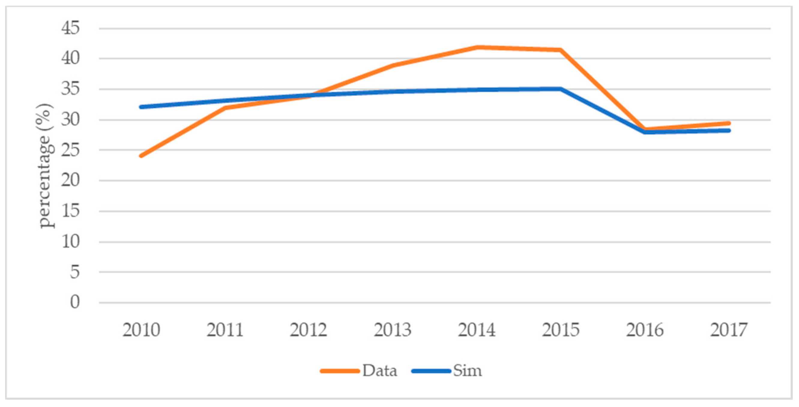
3.2.2. Coral Reef Coverage Dynamics

Coral is a benthic organism which lives as colonies to form a reef covering the bottom of the sea. To model the complex coral reef ecosystem, identifying the indicators of reef state that are most relevant for reef managers, such as coral and algae coverage, as well as the fish population, is essential [26]. In this habitat, coral reefs compete with macroalgae for unoccupied space, while fish, especially herbivorous ones, graze on macroalgae [27].

As a management tool, ecosystem models need to be simplified to improve their applicability, because a complex model requires detailed information that is usually limited in particular areas [28]. Therefore, the coral reef coverage dynamics in this study makes several assumptions. First, coral (C) and macroalgae (M) have a constant growth rate, with the macroalgae growth rate (g_M) exceeding that of the coral (g_C). Their growth is proportional to the existing cover of adults. However, coral also expands through a constant regeneration rate (r_C) determined by an external import of coral propagules which is independent of the local cover of adults. It reflects demographically open populations with the dispersal of juvenile stages. Second, the mortality of coral is represented by a constant decay rate (d_C) and that of macroalgae by a grazing rate (z_M), which depends on fish population dynamics. Lastly, the carrying capacity for coral and macroalgae (K_CM) is indicated by the core zone and rehabilitation zone of Pieh marine park, covering 1818.6 ha, while the area without coral and macroalgae in those zones is termed unoccupied space (S). From a system dynamics perspective, those relationships are best written as:

$$\frac{dC}{dt}=\left(r_C+g_C\times \raisebox{1ex}{$C$}\!\left/ \!\raisebox{-1ex}{$K_{CM}$}\right.\right)S-d_{C}C,$$

(7)

$$\frac{dM}{dt}=\left(g_M\times \raisebox{1ex}{$C$}\!\left/ \!\raisebox{-1ex}{$K_{CM}$}\right.\right)S-z_{M}M,$$

(8)

$$S=K_{CM}-C-M.$$

(9)

The goodness-of-fit of this model was tested by comparing the historical data on coral reef coverage from 2010 to 2017 with the simulation results (Figure 11). There was a coral bleaching event in 2016 that was depicted using a pulse function, instantly decreasing the coral reef coverage that year. The RMSPE value of this model is at only 0.15, while the Theil’s statistics show that the error is caused by unequal variance and covariance (

Table 5. Theil’s statistics of coral reef coverage.

RMSPE	Theil’s Inequality Statistics
	Bias	Unequal Variance	Unequal Covariance
0.15	0.1	0.5	0.4

). Since the purpose of the model is an analysis of long-term behavior extrapolated from a short-term cycle, a substantial value of unequal variance becomes an unsystematic error, and one can conclude that the model is acceptable.

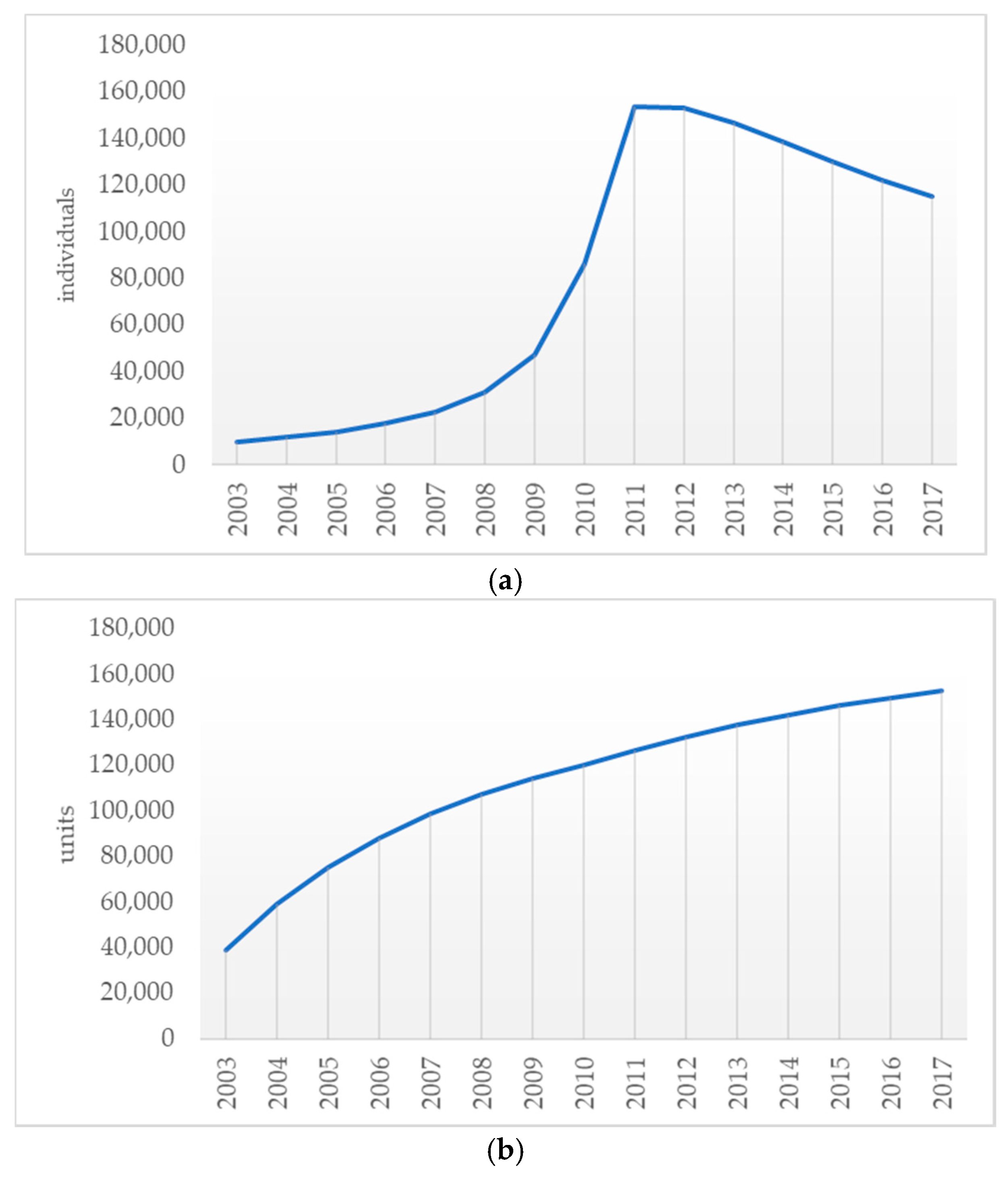
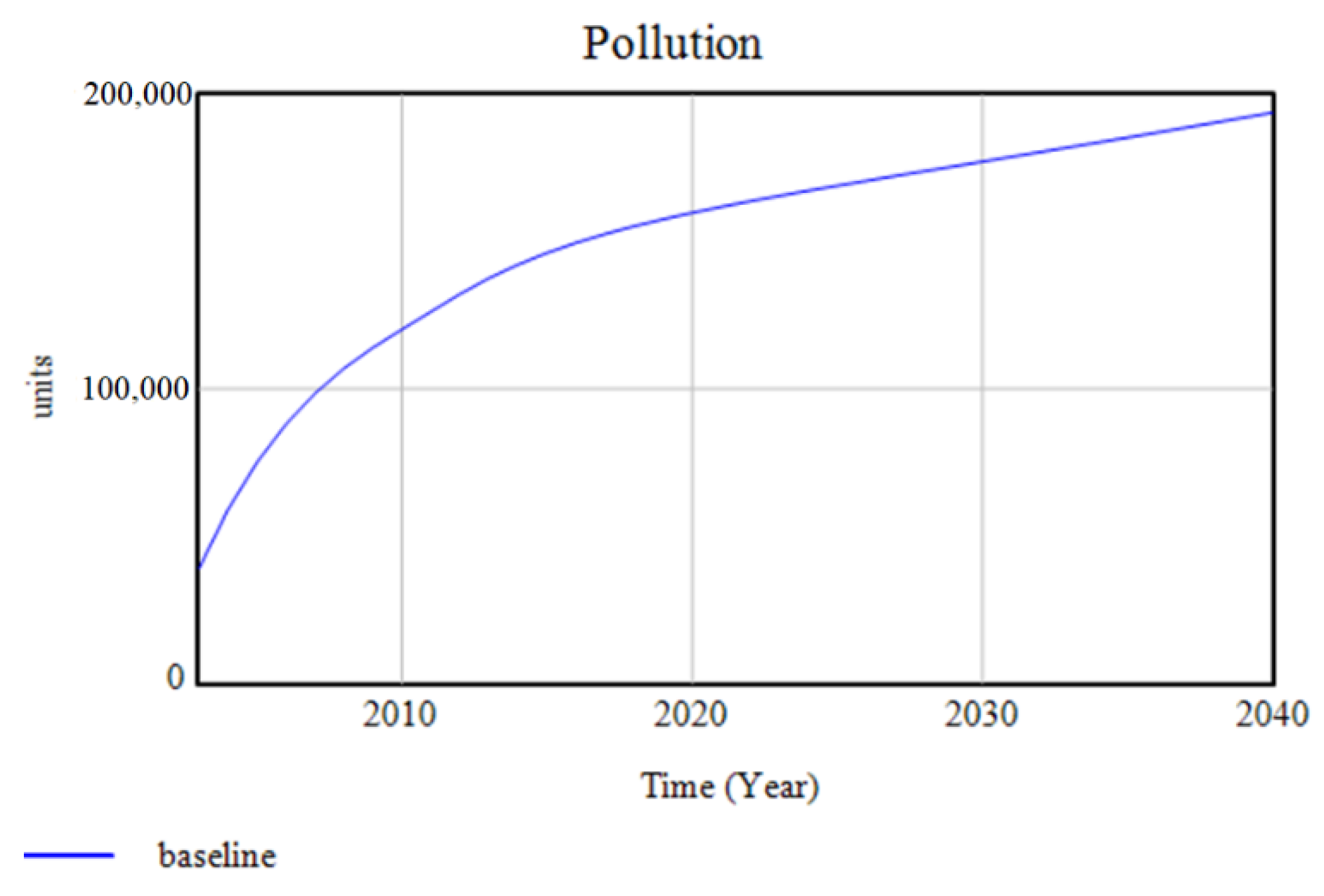
3.2.3. Tourism-Pollution Dynamics

Tourism in the marine and coastal environment depends primarily on the quality of natural resources such coral reef, fish diversity, beaches, and coastal waters [29]. Even if tourism is usually assumed to be a green economy, it also contributes to resource consumption and environmental degradation [30]. Tourism generates waste that can contaminate surface, ground, and marine water, which will further threaten biodiversity and ecosystems and in the long run will degrade the attractiveness of the tourist destination itself [31]. In other words, tourism, pollution, and natural resources are tightly connected through the mediating variable tourism attractiveness. Tourist destinations in good condition attract a large number of tourists, which may lead to overcrowding that, in turn, reduces its attractiveness [31].

Consequently, tourism attractiveness (A) in Pieh marine park is the sum of four factors; the effect of the fish population (Ef), the effect of coral reefs (Ec), the effect of pollution (Ep), and effect of the number of tourists (Et). A non-linear function captures each of these factors (f1, f2, f3, and f4, respectively) which are S-shaped logistic functions closely following this formulation:

$$f_i\left\{x\right\}=\left(B^U-B^L\right)·\left\{1-\frac{\exp \left(slope·\left(x-inflection\right)\right)}{1+\exp \left(slope·\left(x-inflection\right)\right)}\right\}+B^L.$$

(10)

This specification for the logistic function establishes four parameters for each function: (1) the upper bound (BU), a maximum value; (2) the lower bound (BL), a minimum value; (3) the slope of the function; and (4) the inflection point [31]. Therefore, the number of tourists (T) in Pieh marine park can be estimated using the equation below:

$$\frac{dT}{dt}=T\times g_T\times \left(1+A\right),$$

(11)

A = Ef + Ec + Ep + Et.

(12)

According to Pieh management’s tourism plan, tourist growth rate (g_T) is assumed as 11% per year and the carrying capacity of tourists in Pieh marine park is around 85,000 people.

Meanwhile, both tourists and residents generate waste that contributes to the waste loading in Pieh marine park. The waste generated by residents (W_R) rises with the number of residents (R) and the waste produced per person per day (w_r), while the waste generated by tourists (W_T) depends on the number of tourists (T) and the waste produced per tourists per day (w_t). This can be written as:

W_R = R × w_r and W_T = T × w_t.

(13)

Further, the waste treatment facility in Padang Pariaman Regency can manage only 20% of the total waste, with the remainder polluting the environment [32]. The tourism-pollution dynamics in this study produces simulation results for the number of tourists and pollution as in Figure 12, with the assumption that the environment can render around 25% of the pollution harmless. Since there is no historical data on the number of tourists and pollution in Pieh marine park, the goodness-of-fit test was not applied to these dynamics.

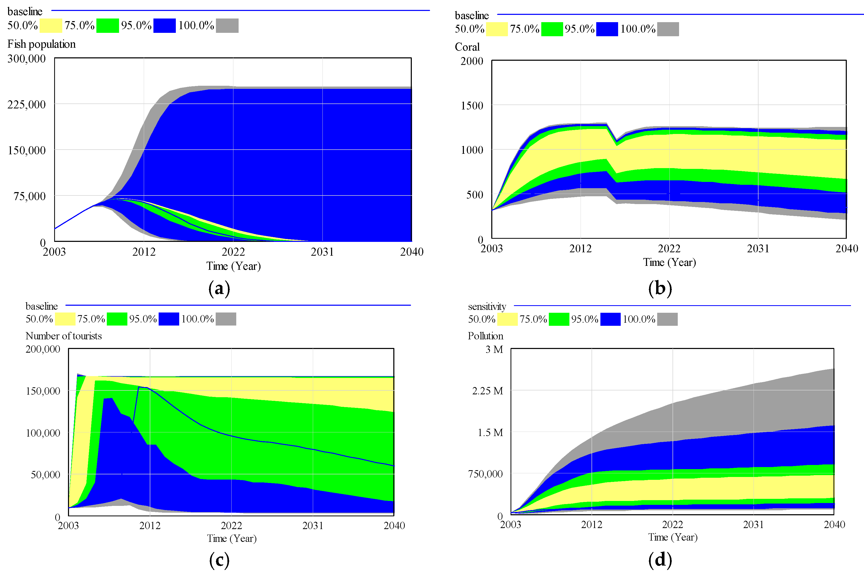
3.2.4. Sensitivity Analysis

The model behavior was investigated by a sensitivity analysis of the simultaneous change in multiple parameters, as listed in

Table 6. Multiple parameters for sensitivity analysis.

Key Variables	Parameters	Minimum	Base	Maximum
Fish population	Total allowable catch	50,000	90,000	150,000
Coral	Coral growth rate	0.1	0.2	0.9
	Coral recruitment rate	0.005	0.01	0.05
Number of tourists	Tourism growth rate	0.01	0.11	0.5
Pollution	Fraction of waste polluting	0.1	0.8	0.9
	Fraction of pollution treatment	0.1	0.25	0.9

. The model was simulated 200 times with independent randomly selected parameter values from a uniform distribution within a specified range. The result of the sensitivity analysis of key variables capturing 50%, 75%, 95%, and 100% confidence interval can be seen in Figure 13. To determine which parameter truly influences the model, the SyntheSim tool in Vensim was used to check the parameters one by one.

It is evident from Figure 13 that the model is robust regarding coral, the number of tourists, and pollution variables, and that simultaneous changes in multiple parameters do not change its behavior. For fish population, a total allowable catch threshold of 62,500 tons changes the model behavior from declining to inclining. Thus, the model is robust enough as only one parameter changes its behavior.

4. Discussion

4.1. Sustainability Assessment

In Pieh marine park, indicators for renewable resources would be fish population dynamics and coral reef. Since economic activities in Pieh marine park do not use non-renewable resources, the second principle can be considered achieved, while indicators for pollutants would be the accumulation of waste. Following this, all of the indicators can be forecast into the future by using the system dynamics model to determine whether Pieh marine park can sustain economic activities in its area or not.

The simulation projected a decline in both fish population and coral reef coverage from 2020 to 2040, with the fish population reaching zero by 2030. The fish population has displayed a declining trend since 2010, while coral reef coverage began declining in 2020 (Figure 14). This condition is not maintainable according to the first principle of sustainability, due to the higher resource depletion rate than regeneration rate.

Meanwhile, the simulation projected an increase in pollution from 2020 to 2040, indicating that waste loading is higher than waste treatment rate or the capacity of the environment to render waste harmless (Figure 15). Thus, the current pollution loading in Pieh marine park is not sustainable.

A semi-structured interview was conducted with the Pieh marine park management officers to determine whether the results of the simulation were surprising or not. The officers thought the results of the simulation represents what they would expect to happen if there is no intervention from the management.

In conclusion, Pieh marine park cannot sustain economic activities in its area, regarding both renewable resource and pollution indicators. It fails to achieve two main goals of an MPA, which are maintaining marine biodiversity and the functioning of the ecosystem, as well as improving socio-economic conditions by increasing revenue from fisheries production and tourism [7]. Those two goals are closely related because depleting natural resources can limit economic growth [33]. Consequently, maintaining biodiversity and ecosystem function is required in order to achieve improving socio-economic conditions. Therefore, the management of Pieh marine park should increase efforts to maintain natural resources in Pieh marine park. In doing so, both main goals can be achieved, and Pieh marine park will sustain economic activities in its area.

4.2. Management Implications

MPAs are widely accepted as a management tool to maintain natural resources in marine and coastal areas while still supporting economic activities for coastal communities. Applying the sustainability concept in an MPA involves a natural resource-based approach, because natural resources have a rather low degree of substitutability, may increase in value over time, and deliver a multitude of services [34]. The argument in favor of strong sustainability is provided by Daly, which state that natural resources, both renewable and non-renewable, should not decrease over time, while pollutants should decrease over time [14].

Using a system dynamics model developed for Pieh marine park, the following management interventions to improve sustainability were identified: lowering the total allowable catch, coral transplantation, and better waste management. These interventions are tightly linked and cannot operate separately.

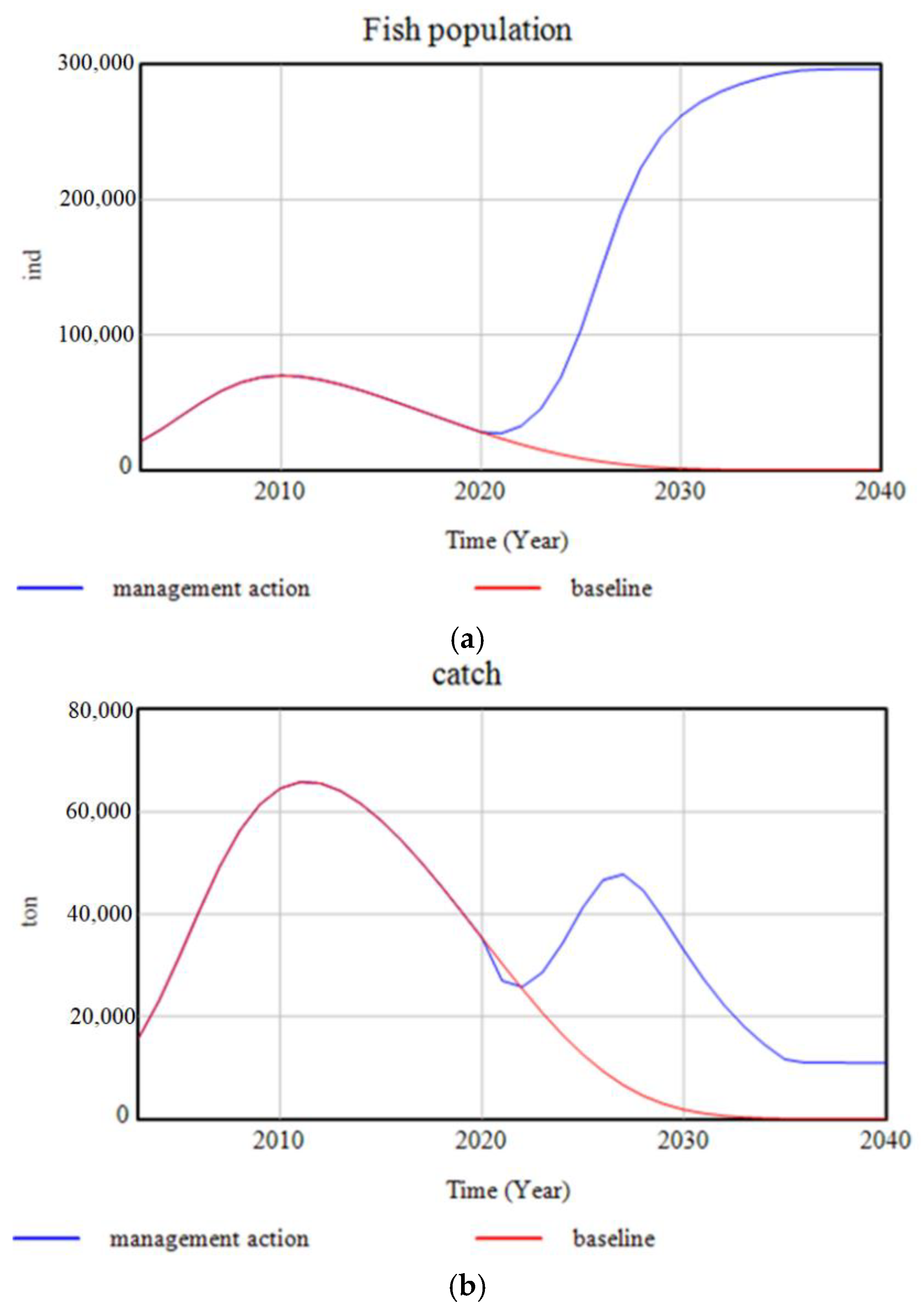
4.2.1. Lowering Total Allowable Catch

MPA establishment is frequently associated with increased fish abundance, biomass, and biodiversity [35]. However, several models of MPAs have shown that effects on fish population depend on dispersal in the larval, juvenile, and adult stages, as well as the size and configuration of reserves and status of the fishery [36]. These models also indicate that the consequences of MPA operation on both fish abundance and yield will depend on the regulations used to limit catch.

In the system dynamics model for Pieh marine park, the total allowable catch is the only variable that can change its behavior. The sensitivity analysis of the model for this variable shows a threshold value of 62,500 tons, which means that lowering this value will change the model behavior regarding fish populations from declining to inclining. A simulation for fish population dynamics showed that by changing the value of the total allowable catch to 11,000 tons results in an increase in the fish population, such that it reaches the carrying capacity in 2040 (Figure 16), while the other variables remain the same. However, this also impacts the fishing catch, which first declines before increasing, decreasing again, and then stabilizing at a TAC value. The simulation result suggests that the TAC should be dynamically adjusted according to the fish population and increases in fishing catch.

The effectiveness of MPAs as a fisheries management tool is likely to be influenced by other regulations. If a significant area is placed in MPAs, the existing total allowable catch will likely need to be reduced to prevent declines in fish abundance [36]. Thus, an MPA should be supported by other regulations to effectively achieve its goals. In Pieh marine park, a dynamic total allowable catch could be an alternative management strategy. In doing so, Pieh marine park could sustain fishery activities in its area.

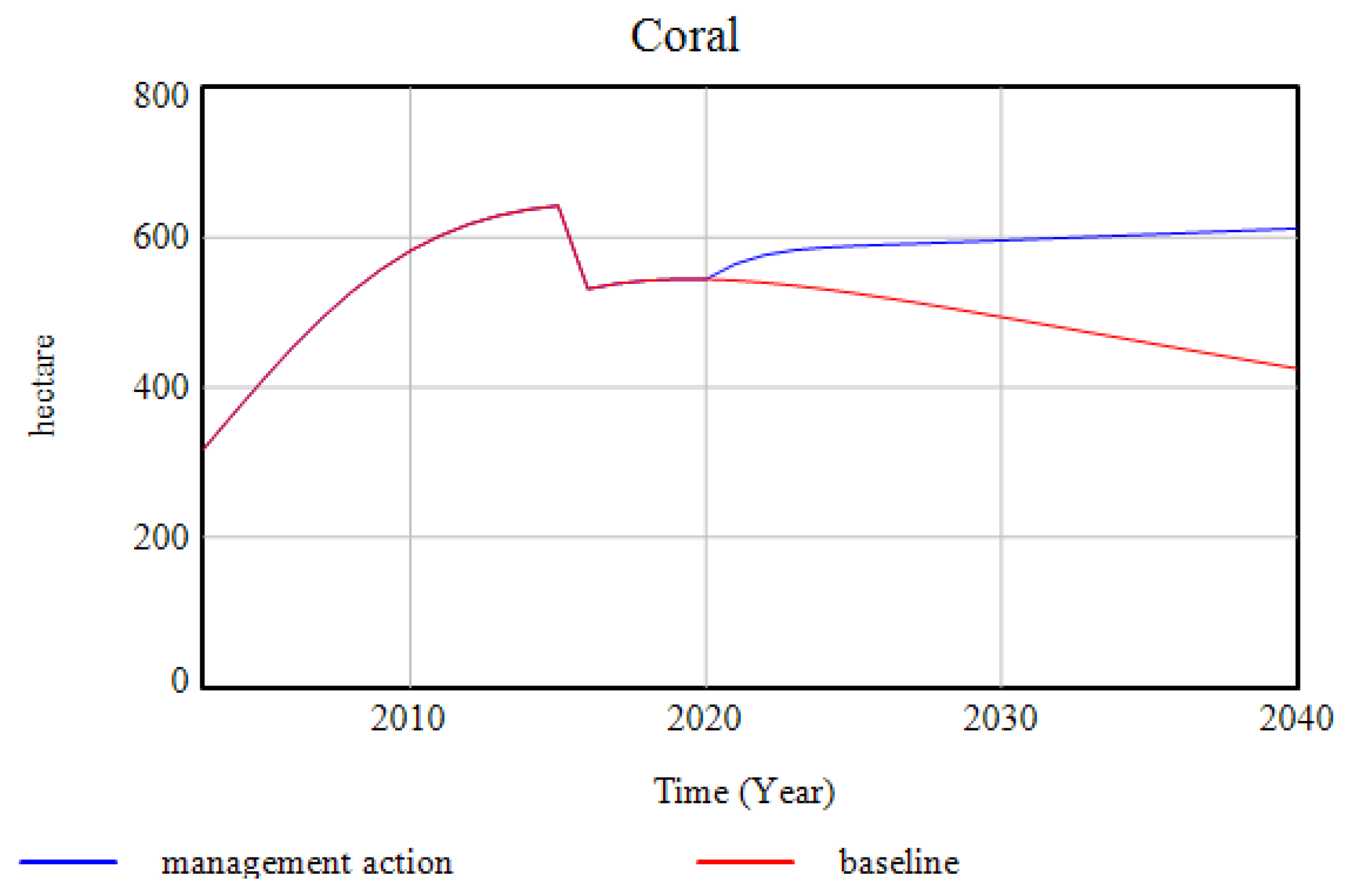
4.2.2. Coral Transplantation

In 2016, there was a coral bleaching event in Pieh marine park that decreased the coral reef coverage from 41.4% to 28.38%. The cause of this disastrous event remains unknown. Coral reefs can take as long as 9–12 years to recover from bleaching disturbance to coral-dominated state [37]. Reef recovery depends on the number of coral fragments that survived and the availability of suitable substrate for the settlement of coral larvae, however, inadequate larval supply may limit coral reef recovery [38]. Coral transplantation has been suggested as a means to rehabilitate reefs by bypassing the critical early stages of coral recruitment, especially on substrata not favorable to larval recruitment or post-recruitment survival [39].

In the system dynamics model for Pieh marine park, coral transplantation is assumed to increase coral recruitment rate to the value of 0.2 in 2020 while the other variables in coral reef dynamics remain the same. The simulation result shows that coral reef coverage would slowly increase, represented by the blue line in Figure 17. This suggests that coral transplantation could increase coral reef coverage as long as the other parameters remain constant. However, coral transplantation cannot be expected to restore coral reefs when conditions causing coral mortality persist [38]. Therefore, environmental monitoring is vital to the success of coral transplantation.

Pieh marine park management has established the core and rehabilitation zones especially for coral transplantation because this area is suitable for coral growth. The level of protection in these zones is strict, with the core zone reserved for conservation and educational activities. While in the rehabilitation zone, only ecotourism activities are allowed. With continual monitoring, coral transplantation in Pieh marine park should be able to sustain ecotourism activities in its area.

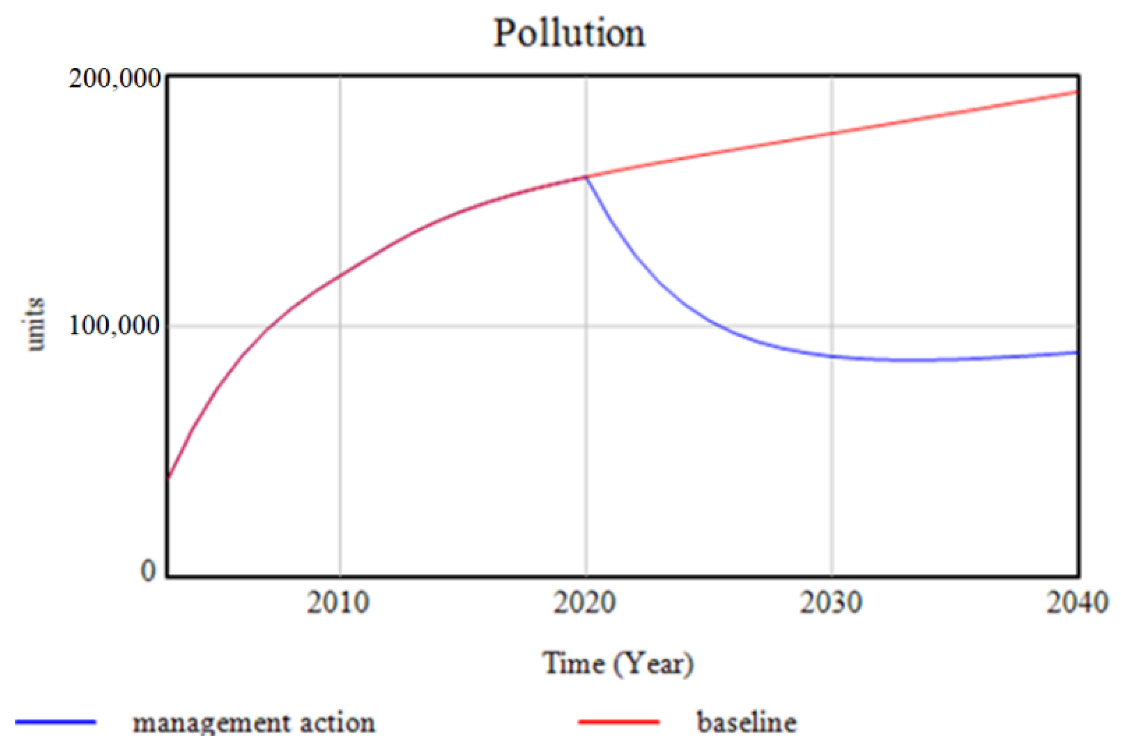
4.2.3. Better Waste Management

The source of waste in Pieh marine park not only comes from the tourists but also from the residents who live in the coastal region in Padang Pariaman regency. The waste treatment facility in Padang pariaman regency can manage only 20% of the total waste and the remainder is disposed of into the environment [32]. Since most of the waste polluting the environment would eventually be transported to the sea, good waste management procedures are crucial in coastal areas.

In modeling better waste management for Pieh marine park, a zero-waste tourism policy could be applied by prohibiting the tourists from bringing food and beverages to the marine park, reducing waste loading from tourists. The local government could also be encouraged to increase the capacity of the waste treatment facility to 60% in 2020, which according to the simulation result, would decrease pollution significantly.

A semi-structured interview was conducted with the Pieh marine park management officers to determine the feasibility of the proposed management interventions. The officers thought the proposed management actions could be feasibly applied. To lower the total allowable catch, it may be necessary to work with fishermen to determine fishing gear limits. Coral transplantation, included in the management plan, would be conducted every year. Promoting zero-waste tourism and increasing waste treatment facility capacity would require regional government involvement.

Even though the level of pollution decreases significantly from 2020 to 2040, a slight increase can be observed at the end of the simulation, as shown by the blue line in Figure 18.

Table 7. The result of simulating a waste polluting environment and the treatment of that pollution.

Year	Polluting (a)	Treatment (b)	(b − a)
2020	21,034	9978	18,944
2021	19,947	35,628	15,681
2022	19,673	32,108	12,435
2023	19,696	29,347	9652
2024	19,826	27,219	7392
2025	19,997	25,597	5599
2026	20,184	24,374	4190
2027	20,378	23,466	3088
2028	20,575	22,803	2227
2029	20,776	22,331	1555
2030	20,978	22,008	1030
2031	21,182	21,802	620
2032	21,389	21,688	299
2033	21,597	21,645	48
2034	21,808	21,658	−150
2035	22,020	21,715	−305
2036	22,235	21,807	−428
2037	22,451	21,926	−526
2038	22,670	22,067	−603
2039	22,891	22,226	−666
2040	23,114	22,398	−716
Average	21,163	24,942

shows the detailed comparison of the waste polluting the environment and the pollution treatment by the environment. On average, pollution treatment is higher than polluting waste, fulfilling the operational principles of sustainability. However, starting from 2034 these principles are no longer met as the level of polluting waste exceeds the pollution treatment. As Daly did not advise on whether to assess variables on an annual or average basis, this study will use the average number for several reasons. First, year by year data do not reflect the behavior of a system. Second, a deviation in the system is usually seen for a specified period and not year by year. Lastly, a management plan is usually designed for a certain period, not annually.

Several limitations and opportunities for model improvement exist. Fishing in tropical regions commonly involves multiple types of gear and multiple species. The fishermen are not selective in fishing, i.e., their catch is not targeting specific species. This study merges all species into one stock because the catch data available in the study area is not grouped by species. However, this approach might not capture the fishery dynamics well; therefore, further study is required. The logistic function for each of the effects on tourism attractiveness in this study is plausible. Even so, the model behavior depends on the slope of the functions and their minimum values. Since specific data on each of the effects are not available, the shape of each function cannot be appropriately estimated. Although sensitivity analysis is conducted over a range of plausible parameters for the functions and explored their impact on model behavior, uncertainty remains. Additional data could be collected using market research methods to estimate these impacts more accurately.

Furthermore, marine ecosystems are complex and dynamic, composed of many biotic and abiotic components that interact with each other [40]. Thus, issues related to marine ecosystem management are regarded as ‘wicked’, meaning that there is no simple answer, but rather a controlled condition in which the solution changes over time [41]. Therefore, the management implications arising from the model generated in this study only forms part of a wider range of solutions.

5. Conclusions

Sustainability assessment of marine protected areas is essential for improving the effectiveness of management efforts. This study focuses on assessing the sustainability of an MPA using a system dynamics approach and then finding the management interventions necessary to achieve sustainability. By using the Pieh marine park as the study site, a system dynamics model was built consisting of four sub-models; fish population, coral reef coverage, tourism, and pollution.

Results of the sustainability assessment suggest that the Pieh marine park cannot sustain economic activities in its area, indicated by the decreasing renewable resource indicators, the fish population and coral reef coverage, as well as increasing pollution indicators. Several management interventions can be applied to achieve sustainability, namely lowering the total allowable catch, coral transplantation, and better waste management. This study also reveals that a time frame is needed when using Daly’s criteria to formulate a sustainability assessment framework.

References

1. IUCN. Establishing Resilient Marine Protected Area Networks—Making It Happen; National Oceanic and Atmospheric Administration and The Nature Conservancy: Washington, DC, USA, 2008.
2. FAO. The State of World Fisheries and Aquaculture; FAO: Rome, Italy, 2016. [Google Scholar]
3. FAO. Marine Protected Areas as a Tool for Fisheries Management. About MPAs. 2009, pp. 1–14. Available online: https://www.imr.no/filarkiv/kopi_av_filarkiv/2006/11/Carl_Gustav_Lundin-IUCNs_work_on_MPAs.pdf/en (accessed on 20 August 2019).
4. WCPA/IUCN. Establishing Marine Protected Area Networks. Making It Happen. A Guide for Developing National and Regional Capacity for Building MPA Networks; National Oceanic and Atmospheric Administration and The Nature Conservancy: Washington, DC, USA, 2007.
5. United Nations. Transforming our world: The 2030 Agenda for Sustainable Development. 2015, pp. 1–35. Available online: https://sustainabledevelopment.un.org/content/documents/21252030%20Agenda%20for%20Sustainable%20Development%20web.pdf (accessed on 20 August 2019).
6. Xu, E.G.B.; Leung, K.M.Y.; Morton, B.; Lee, J.H.W. Science of the Total Environment An integrated environmental risk assessment and management framework for enhancing the sustainability of marine protected areas: The Cape d ’ Aguilar Marine Reserve case study in Hong Kong. Sci. Total Environ. 2015, 505, 269–281. [Google Scholar] [CrossRef]
7. Pomeroy, R.S.; Watson, L.M.; Parks, J.E.; Cid, G.A. How is your MPA doing? A methodology for evaluating the management effectiveness of marine protected areas. Ocean Coast. Manag. 2005, 48, 485–502. [Google Scholar] [CrossRef]
8. Arceo, P.; Granados-Barba, A. Evaluating sustainability criteria for a marine protected area in Veracruz, Mexico. Ocean Coast. Manag. 2010, 53, 535–543. [Google Scholar] [CrossRef]
9. Marques, A.S.; Ramos, T.B.; Caeiro, S.; Costa, M.H. Adaptive-participative sustainability indicators in marine protected areas: Design and communication. Ocean Coast. Manag. 2013, 72, 36–45. [Google Scholar] [CrossRef]
10. Ohl, C.; Krauze, K.; Grunbuhel, C. Towards an understanding of long-term ecosystem dynamics by merging socio-economic and environmental research. Ecol. Econ. 2007, 63, 383–391. [Google Scholar] [CrossRef]
11. Mohamad, D.; Rahman, S.; Bahauddin, A.; Mohamed, B. Tourism sea activities that cause damages towards coral reefs in Sembilan Islands. Tour. Leis. Glob. Chang. 2014, 1, 112–123. [Google Scholar]
12. Mangi, S.; Roberts, C. Quantifying the environmental impacts of artisanal fishing gear on Kenya’s coral reef ecosystems. Mar. Pollut. Bull. 2006, 52, 1646–1660. [Google Scholar] [CrossRef]
13. Keeble, B.R. Brutland Report: Our Common Future. Med. War 1988, 4, 17–25. [Google Scholar] [CrossRef]
14. Daly, H. Ecological Economics and Sustainable Development Selected Essays of Herman Daly; Edward Elgar Publishing: Cheltenham, UK, 2007. [Google Scholar]
15. Collins, R.D. Using inclusive wealth for dynamic analyses of sustainable development: Theory, reflection and application. In Proceedings of the 32nd International Conference of the System Dynamics Society, Delft, The Netherlands, 20–24 July 2014; pp. 1–21. Available online: https://www.systemdynamics.org/assets/conferences/2014/proceed/papers/P1207.pdf (accessed on 8 August 2019).
16. Sterman, J. Business Dynamics: Systems Thinking and Modeling for a Complex World. Review 2000, 34, 324–326. [Google Scholar]
17. Homer, J.; Oliva, R. Maps and models in system dynamics: A response to Coyle. Syst. Dyn. Rev. 2001, 17, 347–355. [Google Scholar] [CrossRef]
18. Lane, D.C. Diagramming Conventions in System Dynamics. J. Oper. Res. Soc. 2000, 51, 241. [Google Scholar] [CrossRef]
19. Pruyt, E. Small System Dynamics Models for Big Issues: Triple Jump towards Real-World Complexity, 1st ed.; TU Delft Library: Delft, The Netherlands, 2013. [Google Scholar]
20. Lopes, R.; Videira, N. Modelling feedback processes underpinning management of ecosystem services: The role of participatory systems mapping. Ecosyst. Serv. 2017, 28, 28–42. [Google Scholar] [CrossRef]
21. Akhtar, M.K. A System Dynamics Based Integrated Assessment Modelling of Global-Regional Climate Change: A Model for Analyzing the Behaviour of the Social-Energy-Economy; University of Western Ontario: London, ON, Canada, 2011; p. 352. [Google Scholar]
22. Sterman, J. Sustaining Sustainability: Creating a Systems Science in a Fragmented Academy and Polarized World. In Sustainability Science: The Emerging Paradigm and the Urban Environment; Weinstein, M., Turner, R., Eds.; Springer Science: New York, NY, USA, 2012; pp. 21–58. [Google Scholar]
23. Dudley, R.G. A basis for understanding fishery management dynamics. Syst. Dyn. Rev. 2008, 24, 1–29. [Google Scholar] [CrossRef]
24. Chang, Y.; Hong, F.; Lee, M. A system dynamic based DSS for sustainable coral reef management in Kenting coastal zone, Taiwan. Ecol. Model. 2008, 211, 153–168. [Google Scholar] [CrossRef]
25. Tan, W.J.; Yang, C.F.; Château, P.A.; Lee, M.T.; Chang, Y.C. Integrated coastal-zone management for sustainable tourism using a decision support system based on system dynamics: A case study of Cijin, Kaohsiung, Taiwan. Ocean Coast. Manag. 2018, 153, 131–139. [Google Scholar] [CrossRef]
26. Melbourne-Thomas, J.; Johnson, C.R.; Fung, T.; Seymour, R.M.; Chérubin, L.M.; Arias-González, J.E.; Fulton, E.A. Regional-scale scenario modeling for coral reefs: A decision support tool to inform management of a complex system. Ecol. Appl. 2011, 21, 1380–1398. [Google Scholar] [CrossRef]
27. Van De Leemput, I.A.; Hughes, T.P.; Van Nes, E.H.; Scheffer, M. Multiple feedbacks and the prevalence of alternate stable states on coral reefs. Coral Reefs 2016, 35, 857–865. [Google Scholar] [CrossRef]
28. Holmes, G.; Johnstone, R. Modelling coral reef ecosystems with limited observational data. Ecol. Model. 2010, 221, 1173–1183. [Google Scholar] [CrossRef]
29. Sealey, S.; Cushion, N. Efforts, resources and costs required for long term environmental management of a resort development: The case of Baker’s Bay Golf and Ocean Club, The Bahamas. J. Sustain. Tour. 2009, 17, 375–395. [Google Scholar] [CrossRef]
30. Mateu-Sbert, J.; Ricci-Cabello, I.; Villalonga-Olives, E.; Cabeza-Irigoyen, E. The impact of tourism on municipal solid waste generation: The case of Menorca Island (Spain). Waste Manag. 2013, 33, 2589–2593. [Google Scholar] [CrossRef]
31. Kapmeier, F.; Gonçalves, P. Wasted paradise? Policies for Small Island States to manage tourism-driven growth while controlling waste generation: The case of the Maldives. Syst. Dyn. Rev. 2018, 34, 172–221. [Google Scholar] [CrossRef]
32. Trihadiningrum, Y. Evaluasi Kapasitas Lahan Tpa Ladang Laweh Di Kabupaten Padang Pariaman Menuju Penerapan Sistem Controlled Landfill. Indones. J. Urban Environ. Technol. 2018, 1, 124–136. [Google Scholar]
33. Romeiro, A.R. Sustainable development: An ecological economics perspective. Estud. Avançados 2012, 26, 65–92. [Google Scholar] [CrossRef]
34. Neumann, B.; Ott, K.; Kenchington, R. Strong sustainability in coastal areas: A conceptual interpretation of SDG 14. Sustain. Sci. 2017, 12, 1019–1035. [Google Scholar] [CrossRef]
35. Halpern, B.; Warner, R. Marine reserves have rapid and lasting effects. Halpern & Wame. Ecol. Lett. 2002, 5, 361–366. [Google Scholar]
36. Hilborn, R.; Micheli, F.; de Leo, G.A. Integrating marine protected areas with catch regulation. Can. J. Fish. Aquat. Sci. 2006, 63, 642–649. [Google Scholar] [CrossRef]
37. Gouezo, M.; Golbuu, Y.; Fabricius, K.; Olsudong, D.; Mereb, G.; Nestor, V.; Doropoulos, C. Drivers of recovery and reassembly of coral reef communities. Proc. R. Soc. B 2019, 286, 20182908. [Google Scholar] [CrossRef] [Green Version]
38. Bowden-kerby, A. Coral Transplantation and Restocking to Accelerate the Recovery of Coral Reef Habitats and Fisheries Resources within No-Take Marine Protected Areas: Hands-On Approaches To Support Community-Based Coral Reef Management. In Proceedings of the Second International Tropical Marine Ecosystems Management Symposium (ITMEMS 2), Manilla, Philippines, 24–27 March 2003; p. 15. [Google Scholar]
39. Bowden-kerby, A. Low-tech Coral Reef Restoration Methods Modeled after Natural Fragmentation Processes. Bull. Mar. Sci. 2001, 69, 915–931. [Google Scholar]
40. Karkkainen, B.C. Collaborative ecosystem governance: Scale, complexity, and dynamism. Va. Environ. Law J. 2002, 21, 189–243. [Google Scholar]
41. Jentoft, S.; Chuenpagdee, R. Fisheries and coastal governance as a wicked problem. Mar. Policy 2009, 33, 553–560. [Google Scholar] [CrossRef]
Figure 1. Zoning Map of Pieh marine park, Padang Pariaman Regency.
Sustainability 11 04609 g001
Figure 2. The trend of tourism and captive fishery in Padang Pariaman regency from 2003 to 2017. (Source: Padang Pariaman regency in figures). (a) The number of tourists; (b) captive fishery production (in tons).
Sustainability 11 04609 g002
Figure 3. Example of Causal Loop Diagram [19].
Sustainability 11 04609 g003
Figure 4. The cross-impact matrix table of Causal Loop Diagram (CLD) [20].
Sustainability 11 04609 g004
Figure 5. The stock and flow diagram for three conditions of sustainability [22].
Sustainability 11 04609 g005
Figure 6. The hypothetical CLD for Pieh marine park.
Sustainability 11 04609 g006
Figure 7. The verified CLD for Pieh marine park.
Sustainability 11 04609 g007
Figure 8. The system dynamics model of Pieh marine park. Links indicated by orange lines are for fishery dynamics, green lines for coral reef dynamics, blue lines for tourism dynamics, and red lines for pollution dynamics.
Sustainability 11 04609 g008
Figure 9. The exponential graph of the number of fishing gears.
Sustainability 11 04609 g009
Figure 10. Comparison of simulated and actual catch data.
Sustainability 11 04609 g010
Figure 11. Comparison of simulated and actual coral reef coverage data.
Sustainability 11 04609 g011
Figure 12. The simulation result of tourism-pollution dynamics across years, with: (a) the number of tourists; (b) pollution.
Sustainability 11 04609 g012
Figure 13. The sensitivity analysis result of key variables; (a) fish population (biomass); (b) coral (hectares); (c) number of tourists (individuals); (d) pollution (dimensionless).
Sustainability 11 04609 g013
Figure 14. The simulation results for renewable resource indicators in Pieh marine park over time. (a) Fish population; (b) coral.
Sustainability 11 04609 g014
Figure 15. The simulation results for pollution indicators in Pieh marine park over time.
Sustainability 11 04609 g015
Figure 16. Lowering total allowable catch to 11,000 tons changes the fish population (a) and fishing catch, Fish population; (b) trend from 2020, Fish catch.
Sustainability 11 04609 g016
Figure 17. Increasing the coral recruitment rate to 0.2 from 2020 onwards changes the trend of coral coverage.
Sustainability 11 04609 g017
Figure 18. The change in pollution from 2020 due to decreasing waste discharge rate from tourists to zero and increasing waste treatment to 60%.
Sustainability 11 04609 g018