Rural Poverty Identification and Comprehensive Poverty Assessment Based on Quality-of-Life: The Case of Gansu Province (China)

Abstract

Rural poverty has received extensive attention worldwide. Eliminating poverty and achieving common prosperity are the major tasks for China to build a well-off society in an all-round way. Based on the evaluation results of quality of rural life (QRL) and relative poverty index (RPI), this paper identifies and classifies the poor objects using importance–Performance analysis (IPA) method and poverty degree model. The results were as following: (1) QRL has obvious regional differences, and its value gradually decreases from west to east, which is opposite to the spatial distribution pattern of RPI. In areas with high QRL value, the RPI is lower. (2) Fifty counties and districts are clustered in the second quadrant of IPA quadrant map, i.e., Low QRL-High RPI, and the lower quality-of-life corresponds to the higher degree of relative poverty. (3) The coincidence between the poverty-stricken counties and the poverty-stricken counties of the country identified as 84.48% by IPA method, which indicates that the accuracy of poverty delineation based on income is high. (4) Gansu Province is dominated by highly impoverished areas, accounting for 60% of the total number of impoverished counties. The results of comprehensive poverty classification are in line with the actual situation of impoverished counties. In counties with higher CPL, the poverty level is deeper. It is more difficult to get rid of poverty. This study can provide theoretical basis and decision-making reference for the formulation and implementation of Poverty Alleviation Policies in the late stage of underdeveloped areas in western China.

1. Introduction

Poverty is a global issue and a realistic challenge that all countries face during their socioeconomic development [1]. Since the 1970s, numerous poverty problems have arisen with the transformation of Western countries to post-industrial society. These problems mainly occur in rural areas, especially those areas with poor environmental quality, disadvantageous geographical location, and inadequate public services and facilities [2]. The World Bank′s Poverty and Shared Prosperity 2016 stated that there were still 767 million people living in extreme poverty worldwide [3]. Eliminating poverty and achieving social justice and fairness has become the core objective and strategic requirement of the socioeconomic development of all countries [4,5]. In view of this, the study of regional poverty has gradually attracted the attention of scholars and politicians from different countries and regions [4,5]. Many scholars focus on poverty level, regional difference, effectiveness of regional targeting policy, and spatial poverty traps in their research [6]. Besides, various national and regional governmental departments have made plans and proposed strategies to deal with poverty, which provide a basis for formulating regional policies [6,7]. Since the late 1990s, some new trends and features have emerged in the methods, contents and perspectives of poverty research with the detailing of census data, the application of geographic information technology and remote sensing technology, and the development of spatial measurement methods. The understanding of the connotation of poverty has been expanding, from a single income-expenditure perspective to a multidimensional perspective involving health, residence, education and social security [8,9,10,11]. This is conducive to quantifying and understanding poverty, which can provide guidance on the formulation and implementation of regional poverty reduction policies.

China is currently the largest developing country in the world, and the rural poverty has always been the focus of Chinese government in formulating poverty alleviation and development plans and policies [12,13,14]. Since 1978, the Chinese government has successively formulated the 8-7 Poverty Alleviation Plan, Development-oriented Poverty Reduction Program for Rural China (2001–2010), Development-oriented Poverty Reduction Program for Rural China (2011–2020) and other measures, aiming to achieve comprehensive poverty alleviation by 2020. After years of hard work, China′s poverty level has been decreased significantly. The rural poverty population decreased from 250 million in 1978 to 55.75 million in 2015, and the incidence of poverty dropped from 30.7% to 5.7%. Poverty reduction practices have achieved remarkable results and contributed significantly to the world′s poverty reduction [15,16,17].

On the basis of regional poverty theory and research methods, scholars have carried out a series of studies on rural poverty in China, including poverty measurement, poverty causes, poverty targeting, geographical identification of poverty, spatial distribution of poverty, etc. Limited by data collection methods and people′s subjective perception of poverty, income alone has been used for a long time to measure poverty. It is widely believed that poverty is a state in which the income of an individual or family cannot meet their basic needs [18]. In recent years, scholars have tried to define and identify poverty from multiple dimensions. They think that income is not the only indicator of poverty and other objective indicators (such as drinking water, roads and sanitation facilities) as well as subjective indicators (such as feeling of welfare) can also be used to measure poverty [9,10,19].

In fact, poverty population are characterized by not only low income levels but also poor quality-of-life. Quality of rural life (QRL) is an important indicator of rural economic development level and directly related to the interests and well-being of rural residents [20,21,22]. However, with rapid urbanization and industrialization, the urban-rural gap has been expanding, which has become a key factor influencing rural sustainable development and restricting rural poverty alleviation [23,24,25]. Improving the quality-of-life of rural poverty groups is conducive to reducing the class conflict and promoting the construction of a harmonious society. In general, current research on rural poverty in China is mainly based on sociology, economics and political science and is mostly from a single economic perspective or multiple perspectives. Notably, there is almost no poverty research from the perspective of quality-of-life. This study identifies poverty from the perspective of QRL. It enriches the scope of poverty research, makes up for the deficiencies of poverty identification research, and can also be used to verify the accuracy of poverty identification results based on income. In addition, it can analyze poverty situation objectively from the provincial scale with a unified standard to provide objective basis for the rational formulation and implementation of poverty alleviation strategy. The measurement methods of poverty have also developed with the deepening of poverty research. They have experienced the evolution from single index to multi-dimensional indicators such as health, education and living standards. They mainly adopt axiomatic method, information theory method, double boundary method, input–output method, quantitative analysis method and so on [26]. However, most of these methods are applicable to specific spatial and temporal backgrounds. They require high data quality or have poor ability to interpret reality. It is difficult to popularize them widely in China. The quality-of-life index makes up for the shortcomings of poverty measurement methods in the past, and helps to quantify and understand poverty more deeply, thus guiding the formulation and implementation of poverty reduction policies in the region.

Gansu Province, which is an underdeveloped area in China, has relatively backward economic development level and low per capita income. This is relateive to many factors, such as history, nature and geography. 66.67% of the counties (cities and districts) in Gansu Province belong to poverty counties, and most of them are located in Liupanshan, Qinba Mountains and Tibetan areas, where the three major countries are concentrated and connected with special difficulties. The incidence of poverty is the second highest in China, second only to Tibet, with 7.9% of the country′s total poor. Therefore, the main characteristics of poverty in Gansu Province are the large number of poor people, the deep degree of poverty, the large area of poverty, the lagging construction of agricultural infrastructure and the fragile ecological environment [27]. This will also be the key and difficult point for China to realize a well-off society in an all-round way in 2020. In this paper, the 87 counties of Gansu Province of China were taken as counties. the QRL and relative poverty of counties were assessed. Then, importance–Performance analysis (IPA) was used to identify poverty objects on a county scale. On this basis, a comprehensive poverty level model was constructed and used to quantify the comprehensive poverty levels of poverty counties, showing the difficulty of poverty alleviation in rural areas of Gansu Province. The results provide a theoretical basis for formulating poverty alleviation and development policies for China′s western underdeveloped regions and achieving the 2020 poverty alleviation goal of China.

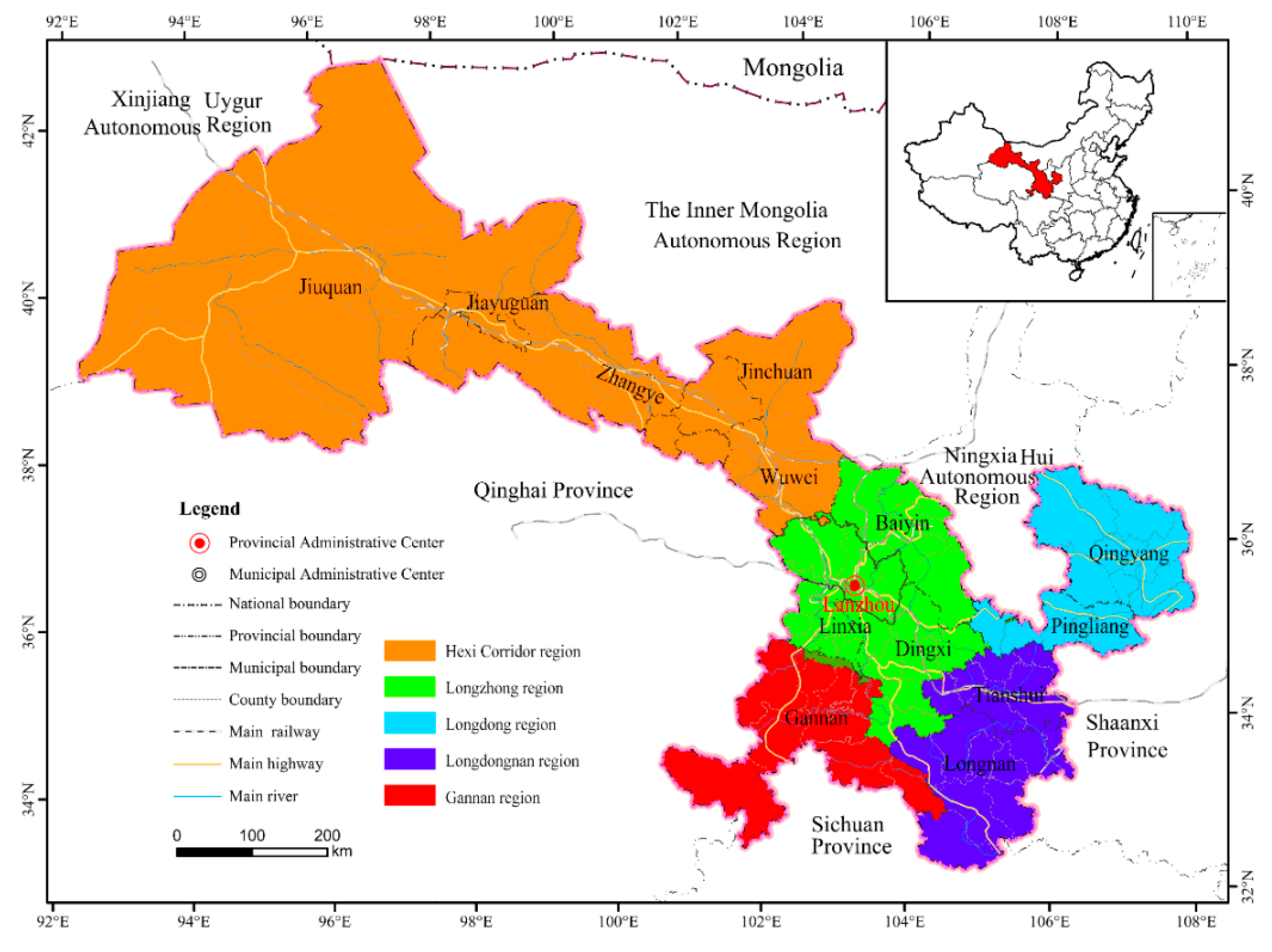
2. Overview of Study Region

Gansu Province is located in western inland China (Figure 1). The total area of the province is 425,800 km², accounting for 4.72% of the total area of the country (Data from Gansu Provincial Natural Resources Department: http://zrzy.gansu.gov.cn). The terrain tilts from southwest to northeast. Since Gansu Province is located in inland China, it is difficult for warm and humid air currents from oceans to reach this region. Precipitation is infrequent and the climate in most areas is dry. Overall, Gansu Province has a continental temperate monsoon climate.

Gansu Province has jurisdiction over 14 cities (including prefectures) and 87 counties (including districts and county-level cities). It can be divided into five regions: Hexi Corridor region (Jiuquan City, Jiayuguan City, Zhangye City, Jinchang City and Wuwei City), Longzhong region (Lanzhou City, Dingxi City, Baiyin City, and Linxia prefecture), Longdong region (Pingliang City and Qingyang City), Longdongnan region (Tianshui City and Longnan City), and Gannan region (Gannan prefecture). Poverty areas are widely distributed in Gansu Province. According to the criteria of poverty-stricken counties in China [28], the average per capita income is less than 1300 yuan, the average per capita income in old areas and minority frontier areas is less than 1500 yuan, per capita GDP is less than 2700 yuan, and per capita financial income is less than 120 yuan. The poverty-stricken counties in Gansu Province are classified according to the criteria. There are a total of 75 poverty counties identified in the province, among which 58 poverty counties are of high poverty and 15 poverty counties are of relatively low poverty. In these poverty counties, there are 6220 poverty villages, 1 million poverty households and 4.17 million poverty population [29].

In 2017, the gross domestic product (GDP) of Gansu Province was 7677 billion yuan and per capita GDP was 29,326 yuan. The GDP of Gansu Province increased from 2010 to 2017, with an annual average increase rate of 10.58%, higher than that of the country during the same period. The population of Gansu Province accounted for 1.89% of the total population of the country, whereas its GDP accounted for only 0.93% of that of the country, social fixed asset investment accounted for 0.89% of that of the country, and general public budget revenue accounted for only 0.48% of that of the country. Gross agricultural product and the yields of main agricultural products both accounted for about 2.0% of those of the country [30].

3. Data Sources and Research Methods

3.1. Data Sources and Preprocessing

The 87 counties of Gansu Province were taken as evaluation units. The basic data about population, income and expenditure, living conditions and cultural life, infrastructure, as well as public services that characterize QRL were derived from Gansu Province Development Yearbook 2017, Gansu Province Rural Yearbook 2017, China Statistical Yearbook 2017 and China Rural Yearbook 2017.

The initial data is normalized to eliminate the effect of dimension and numerical size on the results. In this paper, we choose the max-min normalization method, which maps the original data through linear changes at a specific interval [0,1]. The method requires that the data have the determined maximum and minimum values [31,32]. Because the data used in this paper has the characteristics of the fixed maximum and minimum values, and the direction of the data is inconsistent, we choose the max-min standardized processing method. The direction of the variable in the process of standardization and the normalization of the variables in different directions are as follows: If the value of an indicator is greater, it is more conducive to the development of the system, then the index is a positive indicator, and the Equation (1) will be used for its standardization. If the value of an indicator is less, it is more favorable to the development of the system, then the index is a negative indicator, and the Equation (2) will be used for its standardization. Equations are as follows:

Positive index:

$$Z_i=\frac{C_i-\min \left(C_i\right)}{\max \left(C_i\right)-\min \left(C_i\right)}$$

(1)

Negative index:

$$Z_i=\frac{\max \left(C_i\right)-C_i}{\max \left(C_i\right)-\min \left(C_i\right)}$$

(2)

where C_i and Z_i are the initial and standardized values of the ith index of a county, respectively; the max(C_i) and the min(C_i) are the maximum and minimum values of the ith index, respectively.

In addition, in order to reduce the influence of subjective factors on evaluation results, coefficient of variation was used to assign weight to each index. The procedures are as follows:

$${\delta }_i=\frac{D_i}{{\overline{Z}}_i}$$

(3)

where δ_i, D_i, $\overline{Z_i}$ are the coefficient of variation, mean square error, mean and weight of the ith index, respectively.

$$W_i=\frac{{\delta }_i}{{{\displaystyle \sum }}_{i=1}^n{\delta }_i}$$

(4)

where W_i is the weight of the ith index; δ_i is the coefficient of variation of the ith index; ${\sum }_{i=1}^n{\delta }_i$ is the sum of the variation coefficients of all the variables.

3.2. Research Methods

3.2.1. Assessing QRL

(1) Assessment index system

The assessment index system for QRL is a complex system consisting of multi-attribute, multi-level subsystems. From the perspective of nature-society-economy, this paper fully considered the basic requirements of index selection, including comprehensiveness, purposiveness, scientificity and operability as well as other requirements including policy relevance, multi-dimensional comprehensiveness, research object specificity and data availability. The selection of indices was also in accordance with the standards used at home and abroad for assessing quality-of-life [33,34,35,36]. The final assessment index system involves five aspects including income and expenditure, living conditions and cultural life, infrastructure, public service and social security, and ecological environment. It specifically consists of 3 layers and 21 indices (

Table 1. The assessment index system for QRL in Gansu Province and index weight.

Item Layer	Index Layer	Index Explanation	Index Weight	The Data Source
Income and expenditure B1 (0.1123)	Per capita disposable income of rural residents Z1 (Yuan)	Income earned by rural households after initial and redistribution	0.0564	Gansu Province Rural Yearbook 2017
	Per capita consumption expenditure of rural residents Z2 (Yuan)	Total expenditure of rural residents to meet household consumption in daily life	0.0491	Gansu Province Rural Yearbook 2017
	Engel′s coefficient of rural residents Z3 (%)	The proportion of total food expenditure of rural residents to total personal consumption expenditure	0.0271	Gansu Province Development Yearbook 2017
	Ratio of urban to rural per capita disposable income Z4 (%)	The ratio of urban residents’ disposable income to rural residents’ disposable income	0.0244	Gansu Province Development Yearbook 2017
Living conditions and cultural life B2 (0.2238)	Per capita housing area of rural residents Z5 (m2/person)	Average housing area per person owned by rural residents	0.0483	China Rural Yearbook 2017
	Proportion of cultural entertainment and education expenditure in household consumption expenditure Z6 (%)	An important indicator to reflect the change of rural residents’ consumption structure	0.0296	China Rural Yearbook 2017
Infrastructure B3 (0.1836)	Electricity consumption per 10,000 households Z7 (km·h)	Electricity consumption for social life	0.0644	Gansu Province Development Yearbook 2017
	Tap water usage in rural areas Z8 (%)	Average level of popularity and convenience of rural water supply	0.0194	Gansu Province Development Yearbook 2017
	Access rate of public transportation lines in rural areas Z9 (%)	Coverage Level of Public Transport Team in Rural Areas	0.0362	Gansu Province Rural Yearbook 2017
	Rural broadband coverage Z10 (%)	Response to the level of rural informatization	0.031	Gansu Province Rural Yearbook 2017
	Agricultural mechanization rate Z11 (%)	Indicators for evaluating the utilization of machinery in agricultural production	0.0369	Gansu Province Rural Yearbook 2017
	Agricultural technology popularization rate Z12 (%)	Popularization of scientific and technological achievements and practical technologies in agricultural production	0.0136	China Rural Yearbook 2017
	Rural cable television popularization rate Z13 (%)	Response to the level of rural informatization	0.0525	Gansu Province Development Yearbook 2017
Public services and social security B4 (0.1186)	The number of teachers per 1000 people Z14	Reflecting the development level of rural education	0.0374	Gansu Province Rural Yearbook 2017
	Rate of participation in new rural cooperative medical system Z15 (%)	Reflecting the level of medical assistance in rural areas	0.0673	Gansu Province Rural Yearbook 2017
	Number of hospital beds per 1000 people Z16	Response to the level of rural medical and health facilities	0.1699	Gansu Province Development Yearbook 2017
	Proportion of health care expenditure in household consumption expenditure Z17 (%)	Reflect the proportion of rural medical and health expenditure in the total consumption expenditure	0.0456	China Statistical Yearbook 2017
	Proportion of rural laborers with a high school degree or higher Z18 (%)	Reflecting the education level of rural employees	0.0421	Gansu Province Rural Yearbook 2017
Ecological environment B5 (0.3618)	Rate of centralized treatment of rural domestic garbage Z19 (%)	Popularization of centralized waste disposal in rural areas	0.0261	Gansu Province Rural Yearbook 2017
	Rate of centralized treatment of sewage Z20 (%)	Popularity of rural waste sewage treatment	0.0921	China Statistical Yearbook 2017
	Forest coverage Z21 (%)	The proportion of forest area to total land area.	0.0304	Gansu Province Rural Yearbook 2017

and

Table 2. The Assessment index system for QRL in Gansu Province and statistics of index.

Item Layer	Index Layer	Maximum	Minimum	Average	Standard Deviation
B1	Z1	22,879.070	4496.620	8951.239	4067.423
	Z2	20,876.730	3590.000	8004.559	3509.479
	Z3	0.471	0.206	0.353	0.052
	Z4	0.680	0.240	0.380	0.119
B2	Z5	173.880	7.050	34.658	21.597
	Z6	0.200	0.010	0.098	0.042
B3	Z7	42,956.000	104.080	5573.376	5704.964
	Z8	1.160	0.000	0.788	0.247
	Z9	1.000	0.000	0.619	0.363
	Z10	1.000	0.000	0.644	0.323
	Z11	115.830	44.760	67.983	13.883
	Z12	1.000	0.950	0.993	0.010
	Z13	14.290	0.000	3.178	2.701
B4	Z14	0.340	0.010	0.087	0.047
	Z15	1.000	0.000	0.225	0.246
	Z16	0.560	0.000	0.024	0.067
	Z17	0.740	0.030	0.246	0.159
	Z18	1.000	0.000	0.476	0.324
B5	Z19	100.000	0.000	60.918	25.736
	Z20	0.014	0.000	0.002	0.002
	Z21	0.380	0.040	0.171	0.064

).

(2) Calculating QRL

The index selected in this paper involves many aspects [37], and most of them have complex relationships. Considering the characteristics of the index, the coefficient of variation method is used to determine the weight. This method can identify the importance of the index according to its own differences. The greater the difference, the greater the importance. Equations (1) and (2) were used to standardize the above indices, then the coefficient of variation method was used to determine the weights of indices. Finally, the weighted summation method was used to calculate the QRL of 87 counties.

$$\mathit{QRL}={\sum }_{u=1}^5{W}_u\times B_u={\sum }_{i=1}^4{W}_i\times Z_i+{\sum }_{i=5}^6{W}_i\times Z_i+{\sum }_{i=7}^{13}{W}_i\times Z_i+{\sum }_{i=14}^{18}{W}_i\times Z_i+{\sum }_{i=19}^{21}{W}_i\times Z_i$$

(5)

where QRL is the quality of rural life; B_u is the value of the uth Item; W_u is the weight of the uth Item; Z_i is the standardized value of the ith index; W_i is the weight of the ith index. The greater the value of QRL is, the higher the QRL is.

3.2.2. Assessing Relative Poverty

Defining a poverty line is the most intuitive way to assess the poverty of a region [9,12]. According to the actual situation of Gansu Province and referring to relevant policy documents on the management of poverty alleviation funds in China [38], this paper attempted to measure the level of economic development in a region by measuring the differences between the rural per capita net income/rural per capita GDP/rural per capita fiscal revenue of this region and the corresponding average levels of the province, respectively. On this basis, the relative poverty index (RPI) of a region can be measured. This method is simple, easy to use and can avoid the error caused by incomplete rural statistics in other poverty evaluation methods. The specific procedures are as follows:

$$RP{I}_r=\left(P_{Fr}+P_{Gr}+P_{Ir}\right)/3$$

(6)

$$P_{Fr}=\{\begin{array}{c}\frac{\left(F_k-F_r\right)}{F_k},F_r<F_k\\ 0,F_r\ge F_k\end{array}$$

(7)

$$P_{Gr}=\{\begin{array}{c}\frac{\left(G_k-G_r\right)}{G_k},G_r<G_k\\ 0,G_r\ge G_k\end{array}$$

(8)

$$P_{Ir}=\{\begin{array}{c}\frac{\left(I_k-I_r\right)}{I_k},I_r<I_k\\ 0,I_r\ge I_k\end{array}$$

(9)

where RPI_r denotes the relative poverty index of the rth county, and the greater the value of RPI, the higher the relative poverty level of this county; P_Fr denotes the gap ratio of the rural per capita fiscal revenue of the rth county, F_k is a constant (F_k = 3106 Yuan), indicating the rural per capita fiscal revenue of the province, and F_r is the rural per capita fiscal revenue of the rth county; P_Gr denotes the gap ratio of the rural per capita GDP of the rth county, G_k is a constant (G_k = 27,600 Yuan), indicating the rural per capita GDP of the province, and G_i denotes the rural per capita GDP of the rth county; P_Ir denotes the gap ratio of the rural per capita net income of the rth county, I_k is a constant (I_k = 9951 Yuan), indicating the rural per capita net income of the province, and I_r denotes the rural per capita net income of the rth county.

3.2.3. Spatial Variation Measurement

Spatial autocorrelation is a spatial statistical method that reflects the degree to which a variable is correlated with itself through space. It can be generally divided into the global spatial autocorrelation and local spatial autocorrelation. In this paper, global Moran′s I was used to analyze the spatial distributions of QRL and RPI in Gansu Province.

$$\text{Moran’s} I=\frac{{\sum }_{v=1}^n(x_v-\overline{x}){\sum }_{j=1}^n{W}_{vj}\left(x_j-\overline{x}\right)}{{\sum }_{v=1}^n{\sum }_{j=1}^n{W}_{vj}{\sum }_{j=1}^n{\left(x_v-\overline{x}\right)}^2}$$

(10)

where n is the number of research units; x_v and x_j are observed values of the vth and the jth county respectively; $\overline{x}$ for regional average; W_vj is the spatial weight matrix (1 for spatial neighbor and 0 for non-adjacent region). The value of Moran′s I is in the range of [−1,1]; if I > 0, then there is positive correlation, indicating spatial agglomeration; if I < 0, then there is negative correlation, indicating discrete distribution; if I = 0, then there is no correlation, indicating random distribution. The coefficient of Moran’s I was evaluated using Z-test.

$$Z=\left(I-E\left(I\right)\right)/Var\left(I\right)$$

(11)

where E(I) is the expected value and Var(I) is variance. If Z value is positive and significant, positive spatial autocorrelation exists. If Z value is negative and significant, negative spatial autocorrelation exists. If Z value is 0, then the similar values between regions are distributed randomly.

Getis-Ord $G_v^{*}$ was used to identify the spatial agglomeration characteristics (or hot spots and coldspots) of QRL and RPI.

$$G_v^{*}={\displaystyle \sum }_j^n{W}_{vj}{x}_j/{\displaystyle \sum }_{v=1}^n{x}_v$$

(12)

where x_v and x_j are observed values of the vth and the jth county, respectively; W_vj is the spatial weight matrix (1 for spatial neighbor and 0 for non-adjacent region). If $G_i^{*}$ > 0, then it indicates high-high agglomeration, i.e., a hot spot region; if $G_v^{*}$ < 0, then it indicates low-low agglomeration, i.e., a cold spot region; if $G_v^{*}$ = 0, then it indicates high-low agglomeration.

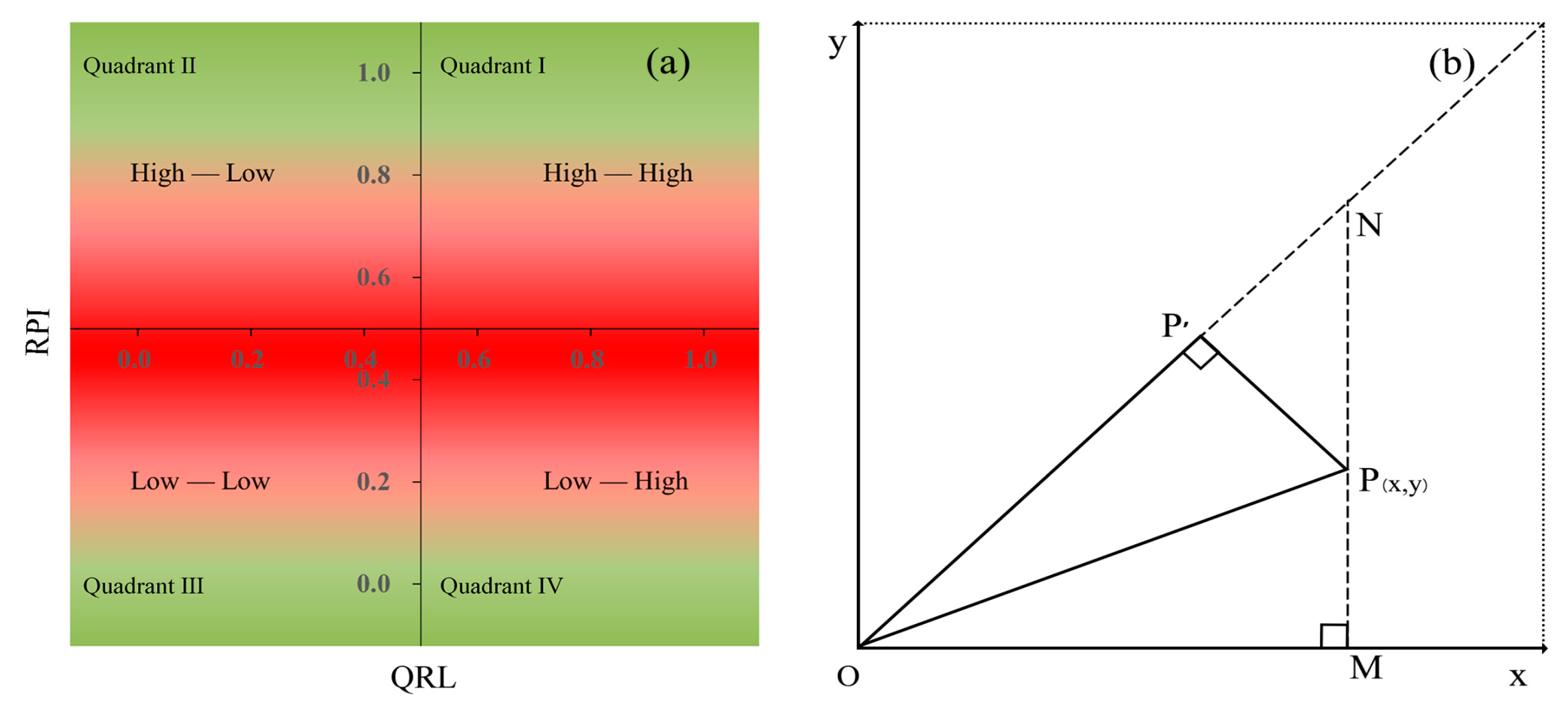
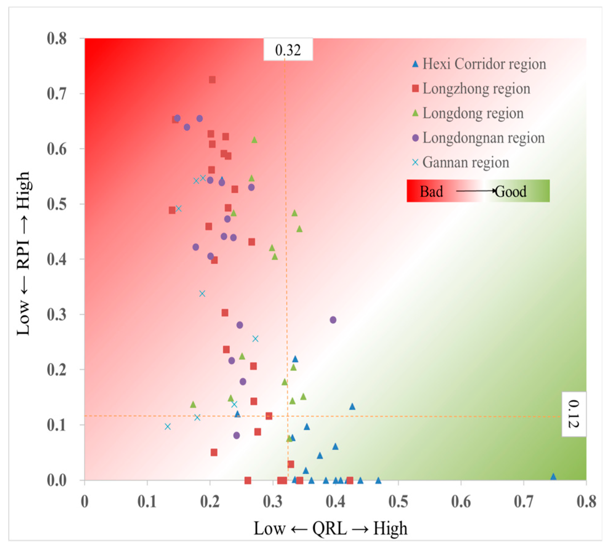
3.2.4. Importance–Performance Analysis

QRL and RPI reflect poverty in terms of living standard and economic development level respectively, but they cannot define the real poverty areas. In recent years, night light remote sensing data and GIS spatial analysis technology have made some progress in the identification of poverty-stricken areas [39], but the defects of the data itself have greatly hindered and weakened the accuracy of night light data in quantitative analysis [40]. On the basis of comprehensive comparison, this study uses the Importance–Performance Analysis (IPA) method to carry out the correlation analysis between the two, and identifies the poverty-stricken areas according to the IPA analysis chart. IPA was first proposed by Martilla and James in 1977 [31]. The basic idea is that a customer′s satisfaction with a product (or service) is determined by the importance that he or she attaches to its attributes and his or her judgment of attribute performance. IPA was first used in the marketing industry to evaluate corporate brands, products and services [41,42]. Due to its simple operation, IPA has currently been widely used in various fields [43,44]. The analysis results are often represented as IPA charts. An IPA chart is usually divided into four areas (Figure 2a): high-high area (the first quadrant), high-low area (the second quadrant), low-low area (the third quadrant) and low-high area (the fourth quadrant). Then reasonable decisions can be made for each area. The horizontal axis of IPA chart represents QRL and the vertical axis of IPA chart represents relative poverty. The QRL values of the 87 counties were arranged in ascending order and the RPI values of the 87 counties were arranged in descending order. Then, the 58th values in both sequences were taken as the coordinates of the origin of IPA chart. On this basis, we studied the distribution of counties in the four quadrants of IPA chart (high RPI-high QRL, high RPI-low QRL, low RPI-low QRL, and low RPI-high QRL). Generally, if a region is characterized by high quality-of-life, then its economic development is good and there is low occurrence of poverty. The counties in the fourth quadrant of IPA chart are examples. If a region is characterized by low quality-of-life and high relative poverty, then this region is considered as a poverty region. The counties in the second quadrant of IPA chart are examples.

3.2.5. Comprehensive Poverty Level

Rural poverty is affected by both QRL and RPI. IPA analysis method is mainly used to identify the poverty-stricken areas, and cannot obtain the specific poverty level of the poverty-stricken areas. This requires that QRL and RPI be “synthesized” into a comprehensive evaluation value through a specific mathematical function to reflect the comprehensive poverty level (CPL). At present, the main methods used are analytic hierarchy process, fuzzy comprehensive evaluation, grey comprehensive evaluation, data envelopment analysis and artificial neural network. Analytical methods [45], etc. Based on the above theoretical analysis, the interaction between QRL and RPI and its internal elements presents an uncertain and complex non-linear relationship. To solve this problem, this study constructs a comprehensive poverty assessment model [46,47]. As shown in Figure 2b, the origin (point O), as defined above, refers to a state in which a region just gets rid of poverty. In this study, the X-axis and Y-axis represent QRL and RPI of the ith county, respectively. Point P shows the QRL and relative poverty of a county. Point P′ is the projection of point P on the diagonal of the first quadrant. The length of line segment OP′ is defined as the comprehensive poverty level (CPL) of the county. The greater the value of OP′, the higher the comprehensive poverty level (CPL). The calculation procedures are as follows:

The length of OP and ON can be calculated according to the Pythagorean theorem:

$$\mathrm{OP}=\sqrt{{\mathrm{OM}}^2+{\mathrm{MP}}^2}$$

(13)

$$\mathrm{ON}=\sqrt{{\mathrm{OM}}^2+{\mathrm{MN}}^2}$$

(14)

According to the calculation method of the triangle area, we can obtain the following equation:

$$S_{△\mathrm{OMN}}=S_{△\mathrm{OPN}}+S_{△\mathrm{OMP}}$$

(15)

$$OM\times MN\times \frac{1}{2}=\mathrm{ON}\times {\mathrm{PP}}^{\prime }\times \frac{1}{2}+OM\times MP\times \frac{1}{2}$$

(16)

The length of PP′ can be calcultaed by the Equati

$$P{P}^{\prime }=\left(OM\times MN-OM\times MP\right)/ON$$

(17)

$$P{P}^{\prime }=\left(OM\times MN-OM\times MP\right)/\sqrt{{\mathrm{OM}}^2+{\mathrm{MN}}^2}$$

(18)

$$P{P}^{\prime }=\left(O{M}^2-OM\times MP\right)/\sqrt{2}\times OM$$

(19)

The length of OP′ can be calculated according to the Pythagorean theorem:

$${\mathrm{OP}}^{\prime }=\sqrt{{\mathrm{OP}}^2-{{\mathrm{OP}}^{\prime }}^2}$$

(20)

$${\mathrm{OP}}^{\prime }=\sqrt{{\mathrm{OM}}^2+{\mathrm{MP}}^2-\frac{{({\mathrm{OM}}^2-\mathrm{OM}\times \mathrm{MP})}^2}{2O{M}^2}}$$

(21)

The length of OM represents the value of QRL, the length of MP represents the value of RPI, and the length of OP′ represents the value of comprehensive poverty level. The final equation for CPL is as follows:

$$\mathrm{CPL}=\sqrt{{\mathrm{QRL}}^2+{\mathrm{RPI}}^2-\frac{{({\mathrm{QRL}}^2-\mathrm{QRL}\times \mathrm{RPI})}^2}{2QR{L}^2}}$$

(22)

4. Results

4.1. Spatial Variation of QRL and Relative Poverty

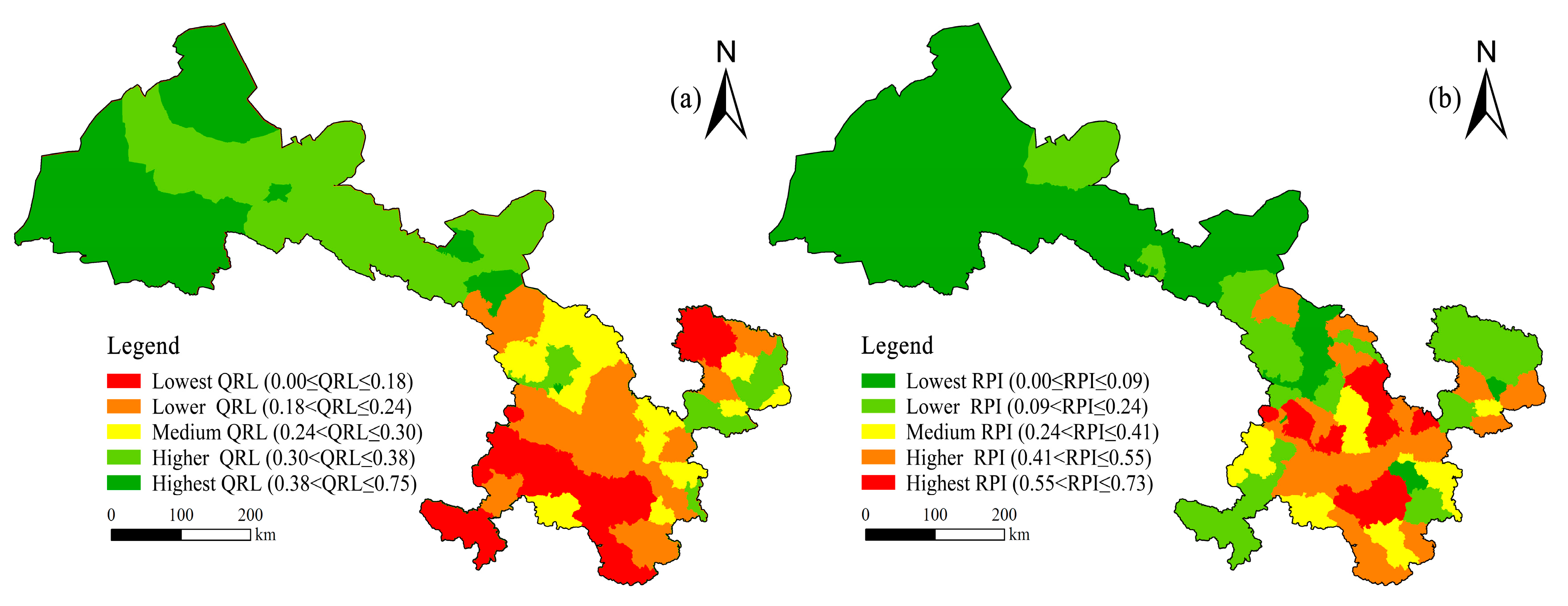
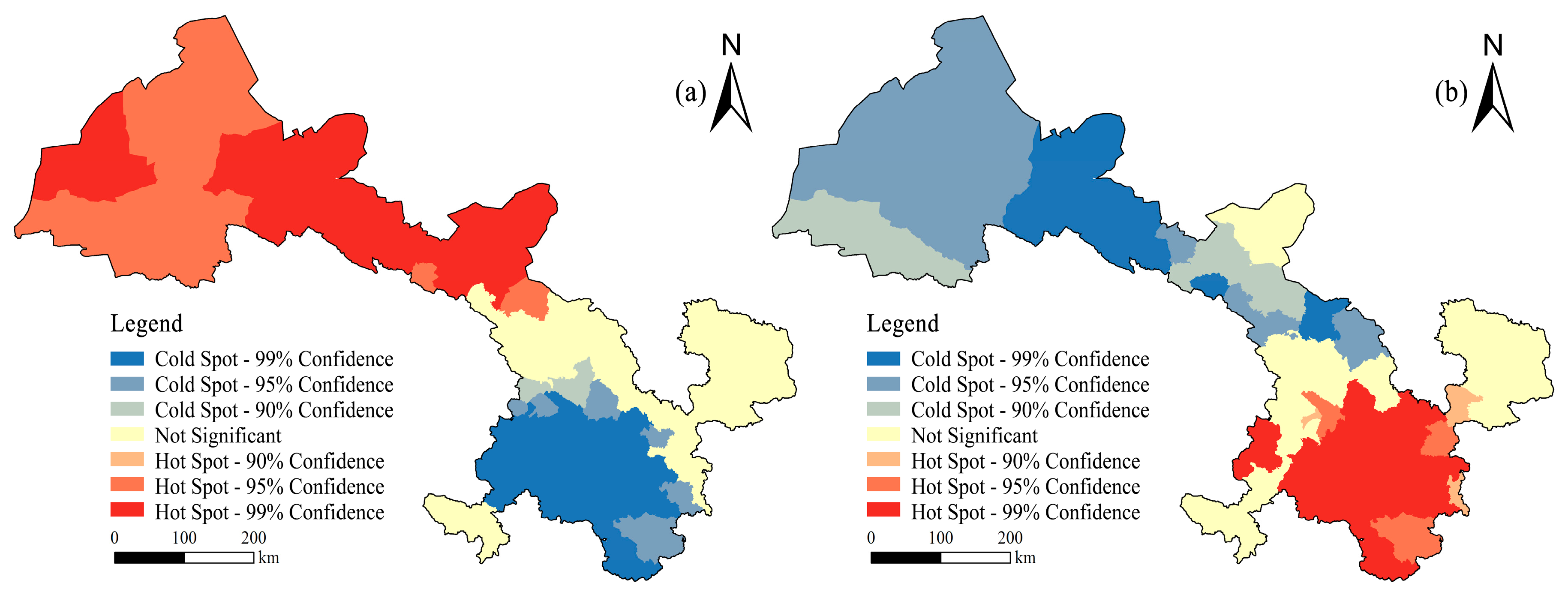
4.1.1. SPATIAL Variation of QRL

The QRL showed significant spatial variation in Gansu Province and the QRL value decreased from west to east (Figure 3a). Hexi Corridor was characterized by the highest QRL, Longzhong region with Lanzhou city as its center was characterized by relatively lower QRL, and Longdongnan, Longnan and Gannan regions were characterized by the lowest QRL. The average value of QRL was 0.2787. There were 35 counties with QRL greater than the average value, accounting for 40.23% of all counties. The counties presented great difference in QRL. Jinchuan district in Hexi Corridor showed the highest QRL of 0.7473. Jiayuguan city in Hexi Corridor showed the second highest QRL, which was about 0.2792 less than QRL value of Jinchuan district. Maqu county in Gannan region showed the lowest QRLof only 0.1322. In Hexi Corridor, 90% counties showed high or relatively high QRL. In both Longzhong and Longdong regions, many counties (50%) showed relatively low QRL. In Longdong and Gannan regions, the majority counties showed relatively high and low QRLe, respectively.

In 2016, the global Moran′s I of QRL was 0.4031 and Z-score was 1.19 (P < 0.01). Therefore, QRL presented positive spatial autocorrelation, spatial agglomeration and spatial heterogeneity. Counties with high QRL tended to be spatially close to counties with high QRL, and counties with low QRL tended to be spatially close to counties with low QRL. The hot spots and cold spots of QRL presented difference between west and east regions (Figure 4a). Specifically, the middle of Hexi Corridor was a primary hot spot of QRL (99% confidence level), and its west and east parts were secondary hot spots of QRL (95% confidence level). The primary cold spot region, including most of Longzhong, Longdongnan and Gannan regions, occupied a larger area than the secondary cold spot.

4.1.2. Spatial Variation of Relative Poverty

The spatial pattern of RPI was opposite to that of QRL (Figure 3b). The RPI values of regions with high QRL values were low. The average value of RPI was 0.2761. The number of counties with RPI less than the average value was 40, accounting for 45.98% of all counties. In 2016, Dongxiang county showed the highest RPI, reaching 0.73. The lowest RPI was found to be 0 and there were 17 counties with RPI of 0. RPI presented significant spatial variation in Gansu Province. In regions to the west of Lanzhou city, 95% of counties showed a RPI less than the average value, which indicates relatively good economic development. In Longzhong and Longdongnan regions to the east of Lanzhou City, counties showed relatively high RPI, and 48.84% of counties showed a RPI higher than the average value. Notably, all counties with high RPI were distributed in these regions. These results indicate poor economic development in these regions.

The global Moran′s I of RPI was 0.3461, and Z-score was 9.09 (P < 0.01). Therefore, RPI presented positive spatial autocorrelation, spatial agglomeration and spatial heterogeneity. The counties with the same level of RPI tended to be spatially close to each other. The spatial pattern of hot spots and cold spots of relative poverty was opposite to that of QRL (Figure 4b). Specifically, the middle of Hexi Corridor was a primary cold spot of the relative poverty (99% confidence level), and its west and east parts were the secondary cold spots of relative poverty (95% confidence level). Longzhong and Longdongnan were majorly hot spots of relative poverty and primary hot spots (99% confidence level) occupied a larger area than the secondary hot spots.

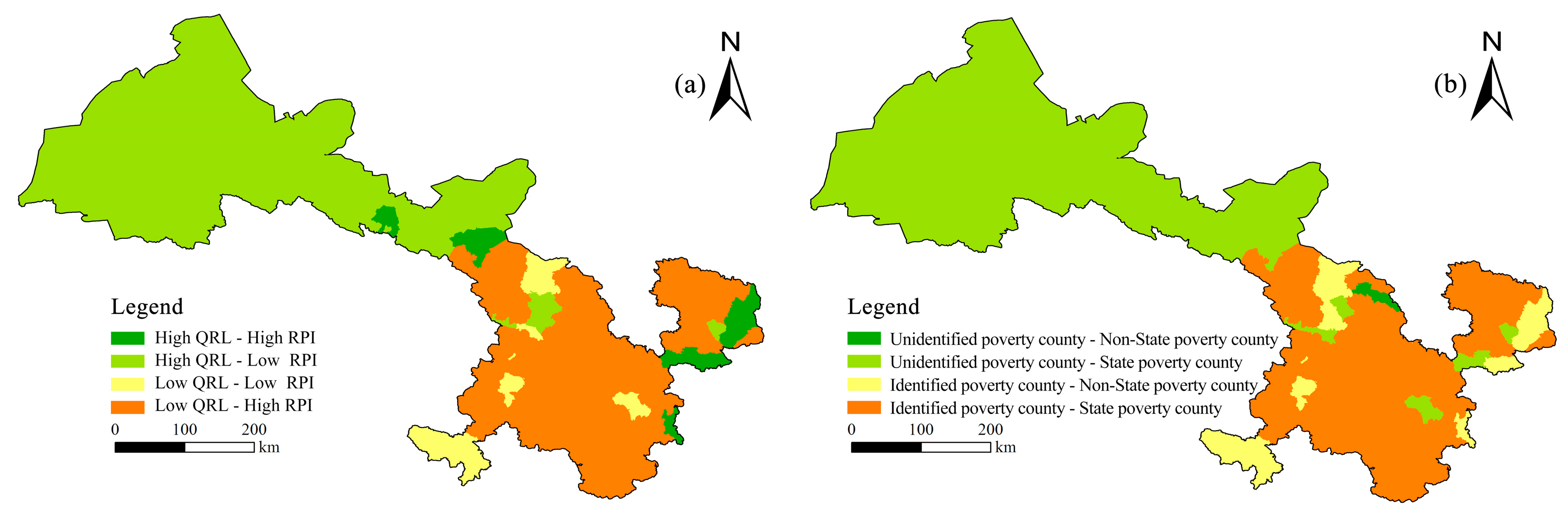
4.2. Identification of Poverty Objects

IPA was performed and the results are shown in Figure 5. The majority (81.61%) of counties were in the second and fourth quadrants. The first and third quadrants represent regions with low QRL and low relative poverty and regions with high quality-of-life and high relative poverty, respectively. There were eight counties in each of the two quadrants. Although the QRL and relative poverty in these counties presented certain inconsistency, their number was small and the accuracy of overall analysis results would not be affected. The second quadrant represents regions with low QRL and high relative poverty. There were 50 counties in this quadrant, accounting for 57.47% of all counties. Among the 50 counties, the majority were located in regions except Hexi Corridor, and especially 87.5% were located in Longdongnan region. The second largest proportion of these counties were located in Gannan region. The fourth quadrant represents regions with high QRL and low relative poverty. There were 21 counties in this quadrant, accounting for 24.14% of all counties. Among these 21 counties, 76.19% were located in Hexi Corridor (

Table 3. Results of identification of poverty objects in Gansu Province.

IPA Quadrants	Hexi Corridor Region	Long zhong Region	Long dong Region	Long dong nan Region	Gan nan Region	In Total
High QRL–High RPI	2	0	5	1	0	8
Low QRL–High RPI	2	19	9	14	6	50
Low QRL–Low RPI	0	5	0	1	2	8
High QRL–Low RPI	16	4	1	0	0	21
In total	20	28	15	16	8	87

). In sum, the regions with high QRL presented low relative poverty, and regions with low QRL presented high relative poverty, indicating good consistency. The 50 counties in the second quadrant satisfied the criteria outlined for poverty counties. Thus, we identified them as poverty counties in this paper.

According to the Development-oriented Poverty Reduction Program for Rural China (2011–2020), a total of 58 counties in Gansu Province were regarded as national poverty counties presenting spatial agglomeration. The spatial overlay analysis of these 58 counties and the 50 poverty counties identified here was shown in Figure 6b. All the identified poverty counties, except Pingchuan district, were national poverty counties identified in the Development-oriented Poverty Reduction Program for Rural China (2011–2020). Therefore, the accuracy of our identification reached 84.48%. The long-term poverty alleviation efforts have gradually achieved results.

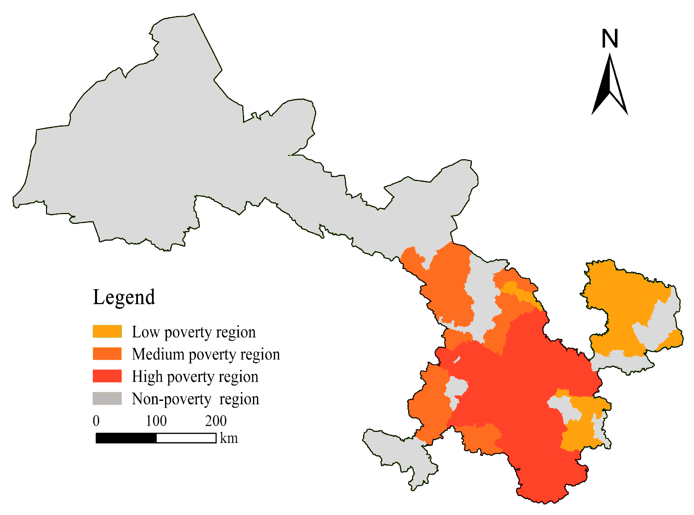
4.3. Comprehensive Poverty Level

Comprehensive poverty level model developed above was used to quantitatively determine the comprehensive poverty level of the 50 poverty counties. According to the spatial distribution characteristics of poverty in Gansu Province, the province was divided into three types of poverty regions and a non-poverty region by using the grouping analysis tool in the ArcGIS 10.2 Mapping Clusters toolset under the condition of ensuring spatial connectione. The three types of poverty regions were low poverty region, moderate poverty region and high poverty region. The number of poverty counties located in the high poverty region was the greatest and reached 30, accounting for 60% of all 50 poverty counties. The numbers of poverty counties located in the low poverty region and moderate poverty region were 11 and 9, respectively, accounting for 22% and 18% of all 50 poverty counties, respectively.

From a spatial perspective(Figure 7), poverty counties were mainly concentrated in the east region of Gansu Province. CPL presented a center-periphery pattern. CPL can also reflect the difficulty of poverty alleviation in poverty counties. It is difficult for counties with high CPL to get rid of poverty. We performed spatial overlay analysis of the classification results based on CPL and 23 deep poverty counties in Gansu Province identified by the government. 17 (73.91%) out of the 23 deep poverty counties were located in the high poverty region of the province. Among the remaining 6 deep poverty counties, 3 were in low poverty region and 3 in moderate poverty region. Therefore, the classification results based on CPL are relatively consistent with the actual situation of Gansu Province. In counties with higher CPL, the poverty level is deeper. It is more difficult to get rid of poverty.

5. Discussion

Poverty identification is the basis for poverty research and poverty reduction decision-making [12,48,49]. Due to its diverse causes, poverty can present different forms in different regions. Social development levels, natural conditions and regional conditions may affect the degree, manifestation and type of poverty [50,51]. These factors may change with time and space. From a perspective of QRL and relative poverty, this paper proposed to use IPA analysis to identify poverty objects. Compared with the case of previous research, our approach based on IPA chart to determine the comprehensive poverty level of a region presents certain innovations, and the results obtained are relatively reliable. Although the method of determining poverty-stricken counties using per capita net income is simple, it is effective in assessing poverty. Because the data used in this paper are more complex and difficult to obtain, considering the dynamic change of poverty, this paper proposes to combine the two methods to identify poverty. The QRL is determined by an individual′s subjective feelings, such as satisfaction with life, inner sense of contentment and self-realization in society [52,53,54]. In addition, it is determined by objective conditions, such as income and expenditure, living conditions and cultural life, rural infrastructure, public services and social security, as well as ecological environment [55,56]. Therefore, QRL is a comprehensive evaluation of one′s living standards. The subjective evaluation is also based on objective conditions. For example, people′s satisfaction with life depends on whether the external objective conditions can make people feel content. Therefore, this study majorly evaluated the QRL according to the objective conditions in rural regions, and paid attention to the relative poverty of regions. The results provide reference for reducing rural poverty.

However, there are still some problems that need further investigation [55]. First, we evaluated the QRL based on the availability of data, including the income, housing, facilities, security and so on in index selection, and excluding natural geographical elements. This should be addressed in future study. Second, due to the limited availability of some data, this paper studied the spatial variation of rural poverty in Gansu Province only in 2016. However, with the implementation of poverty alleviation and development polices, the spatial pattern of poverty and its influencing factors will undergo rapid changes. Future work should focus on the spatiotemporal variation of poverty, identify new factors and problems in the process of poverty reduction, and explore new mechanisms for poverty reduction. Thirdly, the selection of these indicators is based on the research of quality-of-life at home and abroad. According to the index system established by the indicators available in various yearbooks of Gansu Province, it is still difficult to fully extend them to other provinces. In the follow-up study, we will adjust the index system, and extend the study to the West and even the whole country. Fourth, although the comprehensive poverty level model based on IPA chart has achieved good results in this study, it needs to be verified in more regions..

Poverty reduction is a complex systematic and social program [57,58,59,60]. Gansu Province is a major agricultural production area and an important commodity grain base of China, and the poverty problem in Gansu Province cannot be ignored. This region is characterized by spatial agglomeration of poverty, high poverty level and difficult poverty reduction. In most cases, poverty is caused by diseases and the lack of lands. Considering these facts and the natural environment in Gansu Province, future efforts should aim to propose new poverty reduction strategies on the basis of traditional strategies such as development-oriented poverty reduction, specific poverty reduction, industrial poverty reduction and social poverty reduction. For example, a “will enhancement + technology support + personnel training” strategy can be adopted. Specifically, media can be used as a powerful tool to enhance the willingness of people to get rid of poverty [57]. Through such measures as public opinion guidance, skill training and financial support, the development-oriented poverty alleviation and the guarantee-oriented poverty alleviation can be carried out simultaneously. Not only can we guarantee their lives by funding, but also we should promote the development of their industries and create more jobs so as to enhance the poverty-stricken people′s independent poverty alleviation, as in the case of “blood transfusion” poverty alleviation. This can enhance the endogenous motivation of poverty-stricken people to get rid of poverty on their own, and realize the transition from “blood transfusion” of poverty alleviation to “hematopoietic” poverty alleviation. In addition, region-specific poverty reduction strategy should be developed according to the spatial pattern of poverty. Related resources should be carefully allocated to different regions to improve the quality of poverty reduction. We should encourage the innovation of different types of geographic unit production, living and ecological space reconstruction models, approaches and poverty reduction policies to overcome the different spatial poverty disadvantages, and fundamentally solve the problem of regional overall poverty.

6. Conclusions

This paper evaluated the QRL and relative poverty in Gansu Province, and used IPA to identify poverty objects. On this basis, a CPL model was proposed and used to quantitatively determine the CPL of each county. Further, the province was classified into several poverty regions according to the CPL calculation results. In sum, the following conclusions were drawn.

(1) QRL presented significant spatial variation in Gansu Province and decreased from west to east. It showed positive spatial autocorrelation, i.e., spatial agglomeration. Counties with high QRL tended to be spatially close to counties with high QRL, and counties with low QRL tended to be spatially close to counties with low QRL. The spatial pattern of RPI was opposite to that of QRL. Counties with high QRL showed low RPI.

(2) The hot spots and cold spots of QRL presented difference between west and east. The middle of Hexi Corridor was a primary hot spot of QRL, and its western and eastern parts were the secondary hot spots of QRL. The region to the east of Lanzhou city is a cold spot of QRL, and presented a circle layer structure, with center being primary cold spot and periphery being the secondary cold spot. The spatial pattern of hot spots and cold spots of RPI was opposite to that of QRL. Hexi Corridor was majorly a cold spot of PRI. Longzhong and Longdongnan regions were hot spots of RPI, and their peripheral regions were the secondary hot spots of RPI.

(3) Among the 87 counties, 71 (81.61%) were in the second and fourth quadrants of the IPA chart (with QRL as the horizontal axis and RPI the as vertical axis). There were 50 counties in the second quadrant of IPA chart. This represents that these counties showed low QRL and high RPI. Therefore, these counties were identified as poverty counties in this paper. Spatial overlay analysis revealed that 84.48% of these poverty counties were indeed national poverty counties identified by the country. Clearly, our poverty identification method has good accuracy.

(4) Gansu Province can be classified into a low poverty region, moderate poverty region, high poverty region and non-poverty region. Poverty counties in the high poverty region accounted for 60% of all poverty counties, and poverty counties in moderate and low poverty regions accounted for 22% and 18% of all poverty counties, respectively. CPL presented a center-periphery pattern. The central region presented high poverty level, the peripheral northwestern region presented moderate poverty level, and the peripheral southeastern region presented low poverty level. The classification results based on CPL were consistent with the actual situation of the province. In counties with higher CPL, the poverty level is deeper. It is more difficult to get rid of poverty.

References

1. Wang, X.L.; Sabina, A. Measurement of multiple-dimensional poverty in China: Evaluation and policy implication. Chin. Rural Econ. 2009, 12, 4–10. [Google Scholar]
2. Mokomane, Z.; Mokhele, T.; Mathews, C.; Makoae, M. Availability and accessibility of public health services for adolescents and young p eople in south africa. Child. Youth Serv. Rev. 2017, 74, 125–132. [Google Scholar] [CrossRef]
3. World Bank Group. Poverty and shared prosperity2016, taking on inequity. In Poverty and Shared Prosperity Series; World Bank Group: Washington, DC, USA, 2015. [Google Scholar]
4. Sapena, J.; Almenar, V.; Apetrei, A.; Escrivá, M.; Gil, M. Some reflections on poverty eradication, true development and sustainability within cst. J. Innov. Knowl. 2018, 3, 90–92. [Google Scholar] [CrossRef]
5. Ramírez, J.M.; Díaz, Y.; Bedoya, J.G. Property tax revenues and multidimensional poverty reduction in colombia: A spatial approach. World Dev. 2017, 94, 406–421. [Google Scholar] [CrossRef]
6. Tonmoy Islam, T.M. An exercise to evaluate an anti-poverty program with multiple outcomes using program evaluation. Econ. Lett. 2014, 122, 365–369. [Google Scholar] [CrossRef]
7. Wenlue, W.; Qian, R.; Jin, Y. Impact of the ecological resettlement program on participating decision and poverty reduction in southern shaanxi, china. For. Policy Econ. 2018, 95, 1–9. [Google Scholar]
8. Alkire, S.; Apablaza, M.; Chakravarty, S.; Yalonetzky, G. Measuring chronic multidimensional poverty. J. Policy Model. 2017, 39, 983–1006. [Google Scholar] [CrossRef] [Green Version]
9. Pasha, A. Regional perspectives on the multidimensional poverty index. World Dev. 2017, 94, 268–285. [Google Scholar] [CrossRef]
10. Alkire, S.; Roche, J.M.; Vaz, A. Changes over time in multidimensional poverty: Methodology and results for 34 countries. World Dev. 2017, 94, 232–249. [Google Scholar] [CrossRef]
11. Alkire, S.; Seth, S. Multidimensional poverty reduction in india between 1999 and 2006: Where and how? World Dev. 2015, 72, 93–108. [Google Scholar] [CrossRef]
12. Liu, Y.; Liu, J.L.; Zhou, Y. Spatio-temporal patterns of rural poverty in China and targeted poverty alleviation strategies. J. Rural Stud. 2017, 52, 66–75. [Google Scholar] [CrossRef]
13. Guo, Y.Z.; Zhou, Y.; Liu, Y.S. Targeted poverty alleviation and its practices in rural China: A case study of Fuping county, Hebei Province. J. Rural Stud. Corrected Proof (In Press). [CrossRef]
14. Li, E.L.; Deng, Q.Q.; Zhou, Y. Livelihood resilience and the generative mechanism of rural households out of poverty: An empirical analysis from Lankao County, Henan Province, China. J. Rural Stud. Corrected Proof (In Press). [CrossRef]
15. Zhang, Y.; Zhou, X.; Lei, W. Social capital and its contingent value in poverty reduction: Evidence from western china. World Dev. 2017, 93, 350–361. [Google Scholar] [CrossRef]
16. Chen, M.X.; Sui, Y.W.; Liu, W.D.; Liu, H.; Huang, Y.H. Urbanization patterns and poverty reduction: A new perspective to explore the countries along the Belt and Road. Habitat Int. 2019, 84, 1–14. [Google Scholar] [CrossRef]
17. Martin, R. On testing the scale sensitivity of poverty measures. Econ. Lett. 2015, 137, 88–90. [Google Scholar]
18. Filippo, D.; Francesca, C.; Sabrina, G. A new formulation of the dagum distribution in terms of income inequality and poverty measures. Physica A 2018, 511, 104–126. [Google Scholar]
19. Alkire, S.; Santos, M.E. Acute multidimensional poverty: A new index for developing countries. Equity Health Human Dev. 2011, 38. [Google Scholar] [CrossRef]
20. Huang, H.; Liu, S.Q.; Cui, X.X.; Zhang, J.F.; Wu, H. Factors associated with quality-of-life among married women in rural china: A cross-sectional study. Qual. Life Res. 2018, 27, 3255–3263. [Google Scholar] [CrossRef] [PubMed]
21. Janmaimool, P.; Denpaiboon, C. Rural villagers’ quality-of-life improvement by economic self-reliance practices and trust in the philosophy of sufficiency economy. Societies 2016, 6, 26. [Google Scholar] [CrossRef]
22. Tran, T.Q.; Nguyen, C.V.; Van Vu, H. Does economic inequality affect the quality-of-life of older people in rural vietnam? J. Happiness Stud. 2017, 19, 781–799. [Google Scholar] [CrossRef]
23. Bi, A.P. Research Progresses of Rural Regional-System Degradation. Chin. Agric. Sci. Bull. 2014, 30, 112–116. [Google Scholar]
24. Li, H.B.; Zhang, X.L. Spatial Extension in the Context of Urban and Rural Development: Village Recession and Reconstruction. Reform 2012, 1, 148–153. [Google Scholar]
25. Watson, P.; Deller, S. Economic diversity, unemployment and the great recession. Q. Rev. Econ. Financ. 2017, 64, 1–11. [Google Scholar] [CrossRef]
26. Yang, Z.; Jiang, Q.; Liu, H.M.; Wang, X.X. Multi-Dimensional Poverty Measure and Spatial Pattern of China’s Rural Residents. Econ. Geogr. 2015, 35, 148–153. [Google Scholar]
27. Wang, X.W.; He, M.H.; Li, Y.J. Re-selection of Poverty Alleviation Model Based on the Perspective of Spatial Poverty—Taking Gansu as an Example. Gansu Soc. Sci. 2012, 6, 95–98. [Google Scholar]
28. Xinhua News Agency. Fan Xiaojian, Director of the State Council Office of Poverty Alleviation, Explained the New Standard of Poverty Alleviation of 2,300 yuan. Available online: Http://www.gov.cn/jrzg/2011-12/02/content_2009471.htm (accessed on 28 July 2019).
29. Gansu Provincial Poverty Alleviation and Development Office. List of Poor Counties in Gansu Province. Available online: http://fpb.gansu.gov.cn/helpnews/viewnews-14405.html (accessed on 28 July 2019).
30. Gansu Development Yearbook Editorial Board. Gansu Province Development Yearbook 2017; China Statistics Press: Beijing, China, 2017.
31. Sun, H.W.; Lv, C.H.Y.; Qi, A.G.; Cao, G.H.; Han, C.H.L. Research on the principles of data standardization in comprehensive evaluation. Chin. J. Health Stat. 2015, 32, 342–344. [Google Scholar]
32. Liu, J.Y.; Zhang, K.; Wang, G.H. Comparative Study on data standardization methods in comprehensive evaluation. Digit. Technol. Appl. 2018, 36, 84–85. [Google Scholar]
33. Bianca, B.; Maria, G.L.; Marta, M. Urban Quality-of-life and Capabilities: An Experimental Study. Ecol. Econ. 2018, 150, 137–152. [Google Scholar]
34. Sirgy, M.J.; Terri, C. How neighborhood features affect quality-of-life. Soc. Indic. Res. 2002, 59, 79–114. [Google Scholar] [CrossRef]
35. Robert, C.; Brendan, F.; Saleem, A. Quality-of-life: An approach integrating opportunities, human needs, and subjective well-being. Ecol. Econ. 2007, 61, 267–276. [Google Scholar]
36. Zhou, G.H.; Liu, C.; Tang, C.L.; He, Y.H.; Wu, J.M.; He, L. Spatial pattern and influencing factors of quality-of-life in rural areas of Hunan province. Geogr. Res. 2019, 37, 2475–2489. [Google Scholar]
37. Zhong, S.X.; Hu, P.; Xue, X.M.; Yang, S.; Zhu, P.J. Multi-factor comprehensive evaluation model based on the selection of objective weight assignment method. Acta Geogr. Sin 2015, 70, 2011–2031. [Google Scholar]
38. Ministry of Finance of the People’s Republic of China. Central Financial Special Poverty Alleviation Fund Management Measures. Available online: http://fgk.mof.gov.cn/law/getOneLawInfoAction.do?law_id=84519 (accessed on 13 March 2017).
39. Pan, J.H.; Hu, Y.X. Spatial Identification of Multidimensional Poverty in China Based on Nighttime Light Remote Sensing Data. Econ. Geogr. 2016, 36, 124–131. [Google Scholar]
40. Chen, Y.B.; Zheng, Z.H.; Wu, Z.F.; Qian, Q.L. Review and prospect of application of nighttime light remote sensing data. Prog. Geogr. 2019, 38, 205–223. [Google Scholar]
41. Yu, B.; Che, S.; Xie, C.; Tian, S. Understanding Shanghai Residents’ Perception of Leisure Impact and Experience Satisfaction of Urban Community Parks: An Integrated and IPA Method. Sustainability 2018, 10, 1067. [Google Scholar] [CrossRef]
42. Deng, J.; Pierskalla, C.D. Linking Importance–Performance Analysis, Satisfaction, and Loyalty: A Study of Savannah. GA. Sustainability 2018, 10, 704. [Google Scholar] [CrossRef]
43. Wang, X.Y.; Zhu, W.L. Study on the identification of poverty—Stricken areas and the development potential of rural tourism in southern shandong province. Chin. J. Agric. Resour. Reg. Plan. 2018, 39, 269–275. [Google Scholar]
44. Huang, Y.Y. Environmental risks and opportunities for countries along the Belt and Road: Location choice of China’s investment. J. Clean. Product. 2019, 21, 14–26. [Google Scholar] [CrossRef]
45. Zhou, Y.; Guo, Y.Z.; Liu, Y.S. Comprehensive measurement of county poverty and anti-poverty targeting after 2020 in China. Acta Geogr. Sin 2018, 73, 1478–1493. [Google Scholar]
46. Eskildsen, J.K.; Kristensen, K. Enhancing importance–Performance analysis. Int. J. Product. Perform. Manag 2006, 55, 40–60. [Google Scholar] [CrossRef]
47. Deng, W.J. Using a revised importance–Performance analysis approach: The case of Taiwanese hot springs tourism. Tour. Manag. 2007, 28, 1274–1284. [Google Scholar] [CrossRef]
48. Liu, Y.; Xu, Y. A geographic identification of multidimensional poverty in rural china under the framework of sustainable livelihoods analysis. Appl. Geogr. 2016, 73, 62–76. [Google Scholar] [CrossRef]
49. Maleček, P.; Čermáková, K. In-work poverty in the czech republic: Identification of the most vulnerable groups. Proced. Econ. Financ. 2015, 30, 566–572. [Google Scholar] [CrossRef]
50. Glauben, T.; Herzfeld, T.; Rozelle, S.; Wang, X. Persistent poverty in rural china: Where, why, and how to escape? World Dev. (Oxf.) 2012, 40, 784–795. [Google Scholar] [CrossRef]
51. Drèze, J.; Srinivasan, P.V. Widowhood and poverty in rural india: Some inferences from household survey data. J. Dev. Econ. 1995, 54, 217–234. [Google Scholar] [CrossRef]
52. Gazeley, I.; Verdon, N. The first poverty line? Davies’and eden’s investigation of rural poverty in the late 18th-century england. Explor. Econ. Hist. 2014, 51, 94–108. [Google Scholar] [CrossRef]
53. Liang, Z.X.; Hui, T.K. Residents’ quality-of-life and attitudes toward tourism development in china. Tour. Manag. 2016, 57, 56–67. [Google Scholar] [CrossRef]
54. Martilla, J.A.; James, J.C. Importance–Performance analysis. J. Mark. 1997, 41, 77–79. [Google Scholar] [CrossRef]
55. Wu, X.Y.; Qi, X.H.; Yang, S.; Ye, C.; Sun, B. Research on the Intergenerational Transmission of Poverty in Rural China Based on Sustainable Livelihood Analysis Framework: A Case Study of Six Poverty-Stricken Counties. Sustainability 2019, 11, 2341. [Google Scholar] [CrossRef]
56. Ministry of Finance of the People’s Republic of China. Notice on Printing and Distributing the Measures for the Administration of Special Funds for Poverty Alleviation by Finance (2011–2016). Available online: http://www.gov.cn/gzdt/2011-11/29/content_2006260.Htm (accessed on 10 March 2019).
57. Yang, R.; Wen, Q.; Wang, C.; Du, G.M.; Li, B.H.; Qu, Y.B.; Li, H.B.; Xu, J.W.; He, Y.H.; Ma, L.B.; et al. Discussions and thoughts of the path to China’s rural revitalization in the new era: Notes of the young rural geography scholars. J. Nat. Resour. 2019, 34, 890–910. [Google Scholar]
58. Liu, Y.S.; Guo, Y.; Zhou, Y. Poverty alleviation in rural China: Policy changes, future challenges and policy implications. China Agric. Econ. Rev. 2018, 10, 241–259. [Google Scholar] [CrossRef]
59. Yang, Z.; Guo, Y.; Liu, Y.; Wu, W.; Li, Y. Targeted poverty alleviation and land policy innovation: Some practice and policy implications from china. Land Use Policy 2018, 74, 53–65. [Google Scholar]
60. Chen, J.; Wang, Y.; Wen, J.; Fang, F.; Song, M. The influences of aging population and economic growth on chinese rural poverty. J. Rural Stud. 2016, 47, 665–676. [Google Scholar] [CrossRef]
Figure 1. Location map of Gansu Province at China.
Sustainability 11 04547 g001
Figure 2. (a) IPA chart; and (b) schematic of comprehensive poverty level evaluation.
Sustainability 11 04547 g002
Figure 3. Spatial distribution of (a) QRL and (b) RPI in Gansu Province in 2016.
Sustainability 11 04547 g003
Figure 4. Hot spot detection of QRL (a) and RPI (b) in Gansu Province in 2016.
Sustainability 11 04547 g004
Figure 5. Distribution of counties in IPA chart.
Sustainability 11 04547 g005
Figure 6. Identification of (a) poverty objects and (b) spatial overlay analysis results.
Sustainability 11 04547 g006
Figure 7. Classification of Gansu Province into four regions according to CPL calculation results.
Sustainability 11 04547 g007