Development of a Cost Forecasting Model for Air Cargo Service Delay Due to Low Visibility

Abstract

The air cargo market is growing due to the spread of information technology (IT) products, the expansion of e-commerce, and high value-added products. Weather deterioration is one factor with a substantial impact on cargo transportation. If the arrival of cargo is delayed, supply chain delays occur. Because delays are directly linked to costs, companies need precise predictions of cargo transportation. This study develops a forecasting model to predict delay times and costs caused by the delayed arrival of cargo due to severe weather in the air cargo service environment. A seasonal autoregressive integrated moving average (SARIMA) model is developed and analyzed to address delay reductions in cargo transportation. Necessary data are identified and collected using time series data provided by Incheon International Airport Corporation, with an emphasis on monthly data on cargo throughput at Incheon International Airport from January 2009 to December 2016. The model makes forecasts for further analysis. The model stands to provide decision makers with strategic and sustainable insights for cargo transportation planning and other similar applications.

1. Introduction

In the first decades of the 21st century, the air cargo market has grown rapidly due to the spread of information technology (IT) products, the expansion of e-commerce, and high value-added products. The world’s air traffic will increase by 4.7 percent annually over the next 20 years, and it will double by 2035. In order to reduce the delay, airports and airlines can adjust their flight schedules, expand airport terminals, and introduce weather observation equipment to reduce such delays [1]. Cargo exports in South Korea amounted to US $175 billion in 2017, an increase of 30.3% over the previous year. The industry also recorded a high annual growth rate of 8.1% across a preceding period of five years. During that period of growth, wireless communication equipment and computers accounted for 70% of total cargo exports, mainly in semiconductors, and cargo exports of high value-added products such as pharmaceuticals and cosmetics also increased significantly. Among trading partners, Vietnam grew strongly, and China and Hong Kong topped the list. These three countries accounted for 64% of total cargo exports in South Korea during the period of observation [2,3,4].

Experts predict that cargo exports will continue to increase as the demand for semiconductors, IT products, and special cargo expansions on the back of global economic recovery and the growth of the reverse-purchase market. Therefore, Korean exporters have the potential to continue to expand the export of high-end consumer goods by positively utilizing air cargo transportation [5,6].

Air cargo transportation has the advantages of maintaining constant quality in products during transportation with low risks of damage due to a promptness of delivery and supply chain timeliness. However, because air cargo costs are relatively high, air cargo mainly operates in a small sector of transportation centered on IT, high value-added products, and products sensitive to physical environmental conditions. High value-added products, such as semiconductors, computers, and wireless communication devices, are usually transported by air because the longer the period of transportation, the greater the risk of breakage in these types of products. In the case of medicines, cosmetics, or dangerous goods (such as lithium batteries), air transportation is preferred because it allows for greater control over certain aspects of the external environment, including temperature [7,8].

In recent years, as consumers’ desire for rapid delivery has increased and the development of comprehensive logistics has reduced cargo rates in comparison to the past, air transportation has expanded around small consumer goods. As the link between air transport and land transport closes, consumer needs can be met by the rapid delivery of products at lower fares. ICB is the official partner of Cainiao, the logistics company of China’s Alibaba Group. This partnership has made possible the construction of a logistics warehouse close to the airport to shorten the distance between land transportation and air transportation and has allowed for the use of China’s extensive logistics system by way of professional cooperation [9,10].

According to the International Air Transport Association (IATA), freight ton kilometers (FTK) handled by airlines around the world in September 2018 fell 0.3% from the previous month, and global air cargo growth was 2.0% higher than in September 2017 [11,12]. Air cargo volume has been reported to have maintained a robust growth due to strong consumer confidence, investment growth, and e-commerce activity. Additionally, air cargo competition is increased, and cargo market itself is becoming important for a sustainability of the airport industry [13,14]. Delays incur costs, so airlines’ management plan operations to minimize delay time. There are several delays such as weather, internal, passenger/baggage, cargo/mail, handling, technical, damage/failure, operation, air traffic control, and others. There are various reasons to delay, such as due to late arrival (about 40%), air carrier (about 32%), aviation system (about 23%), weather (about 5%) and security (about 0.1%). The weather accounts for about 5% of the total delay, but 58% of the cancellation [15,16]. Thus, weather deterioration around airports has substantial effects on cargo transportation. However, few previous studies have explored predicting delay times and costs caused by weather.

The purpose of this study is to develop a forecasting model to predict delay times and costs caused by the delayed arrival of cargo due to low visibility environments, especially low visibility by fog. Weather deterioration due to low visibility by fog around airports occasionally prohibits the use of airports, potentially causing crises for companies in the global supply chain environment. If the arrival of cargo is delayed, supply chain delays occur. Because delays are directly linked to costs, companies need precise predictions of cargo transportation. Costs that are caused by delay are extra air cargo fuel, air cargo maintenance cost, air crew cost, airport usage cost, and compensation cost. Thus, airport corporation and airline companies need to cooperate to build strategies of airline scheduling, terminal expansions, and weather forecasting facilities for proper cargo transportation in order to minimize the related costs. Thus, this study will provide business decision-makers with strategic insights in order to improve the quality of service and sustainable operations in current airports, airline companies, and other similar settings.

2. Literature Review

2.1. ARIMA Model and Seasonal ARIMA Model

Our method involves a seasonal autoregressive integrated moving average (SARIMA) model, which is used when there are trends and seasonalities in time series data. The SARIMA incorporates seasonal terms in a general autoregressive integrated moving average (ARIMA) model. The ARIMA model combines an autoregressive (AR) model with a moving average (MA) model, starting from the concept that recent observations have a strong influence on future predictions.

The ARIMA model is more suitable for short-term prediction than long-term prediction because it gives more weight to historical observations that are closer to recent times than to the distant past. More recent weight for events observed in the near past means that long-term predictive values obtained from the ARIMA model are less reliable than short-term predictive values. The ARIMA model can also be used to predict seasonal or periodic fluctuations in time series data. The work of Box and Jenkins [17] suggests that an appropriate sample size is required to set up the ARIMA model and that at least 50 observations are required for the sample to be used. Particularly in cases involving seasonal fluctuations, larger samples are required.

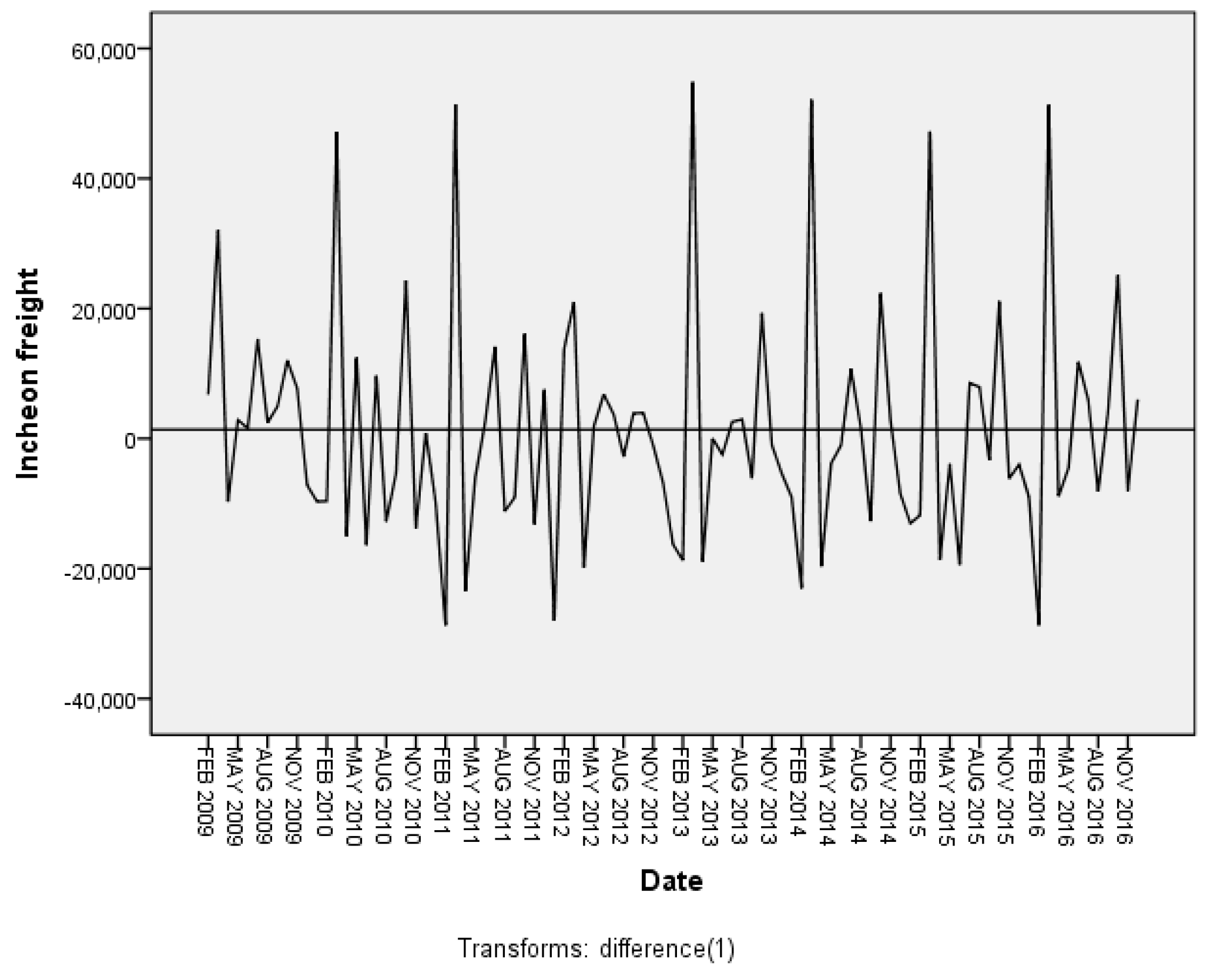
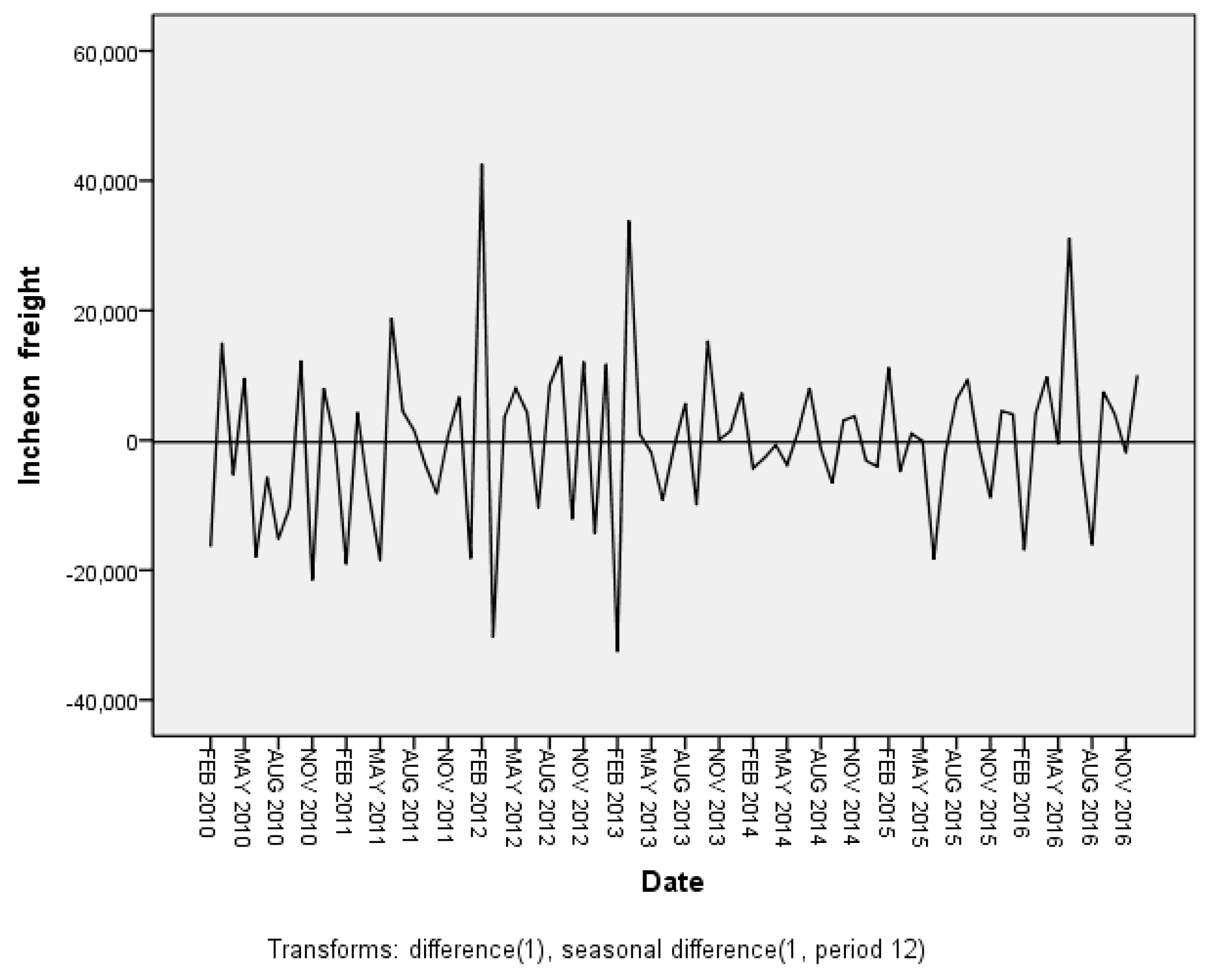
In order to construct the ARIMA model, the first step is to satisfy the stationarity of the average and the variance of data. In the presence of non-stationarity and seasonality, non-seasonal differences (d) and seasonal differences (D) ensure a steady state. The difference is obtained by subtracting the value of a past specific time from the value of the present time point and replacing the value with the new value. Thus, the more the number of times of the difference (d, D), the more the data are damaged.

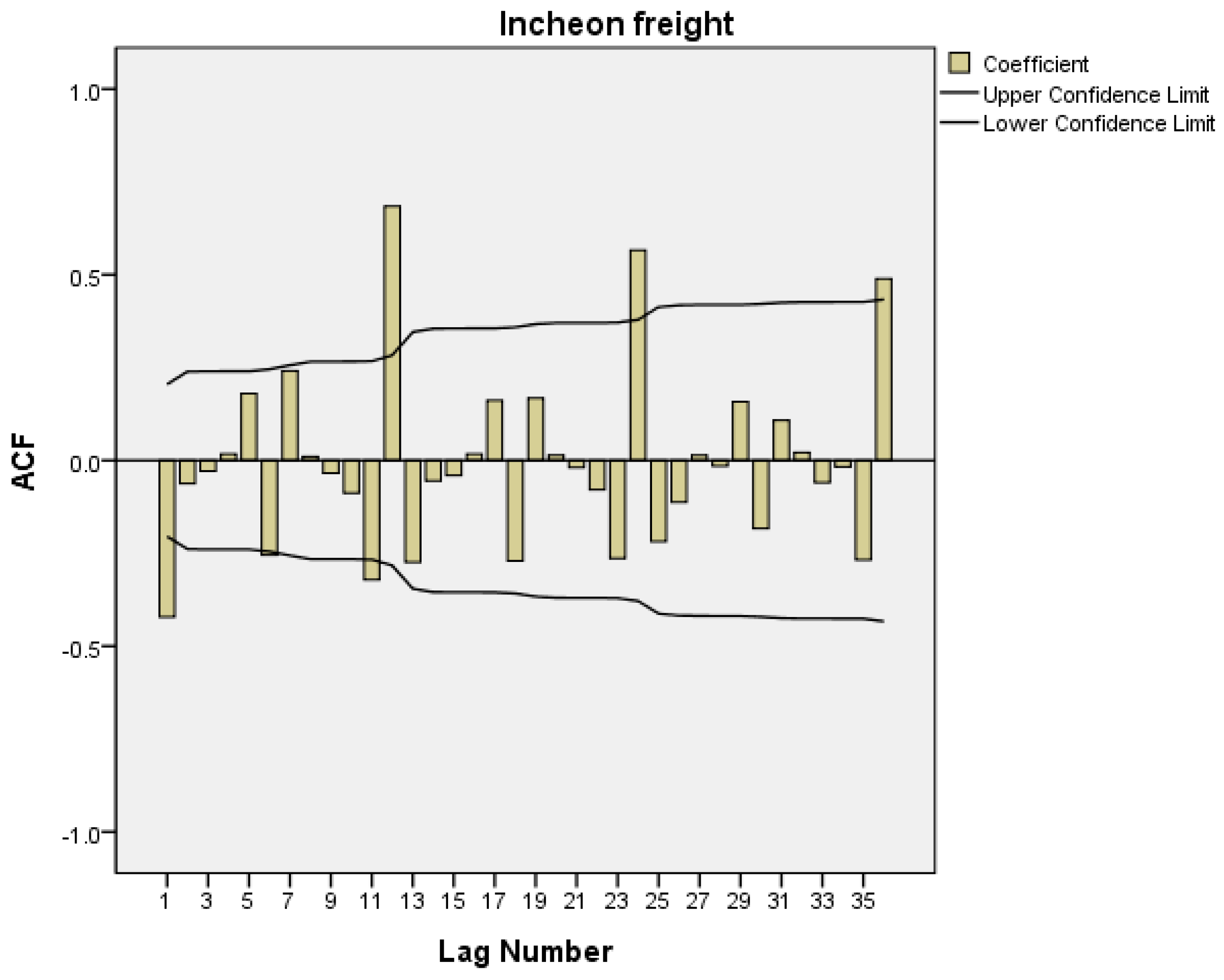
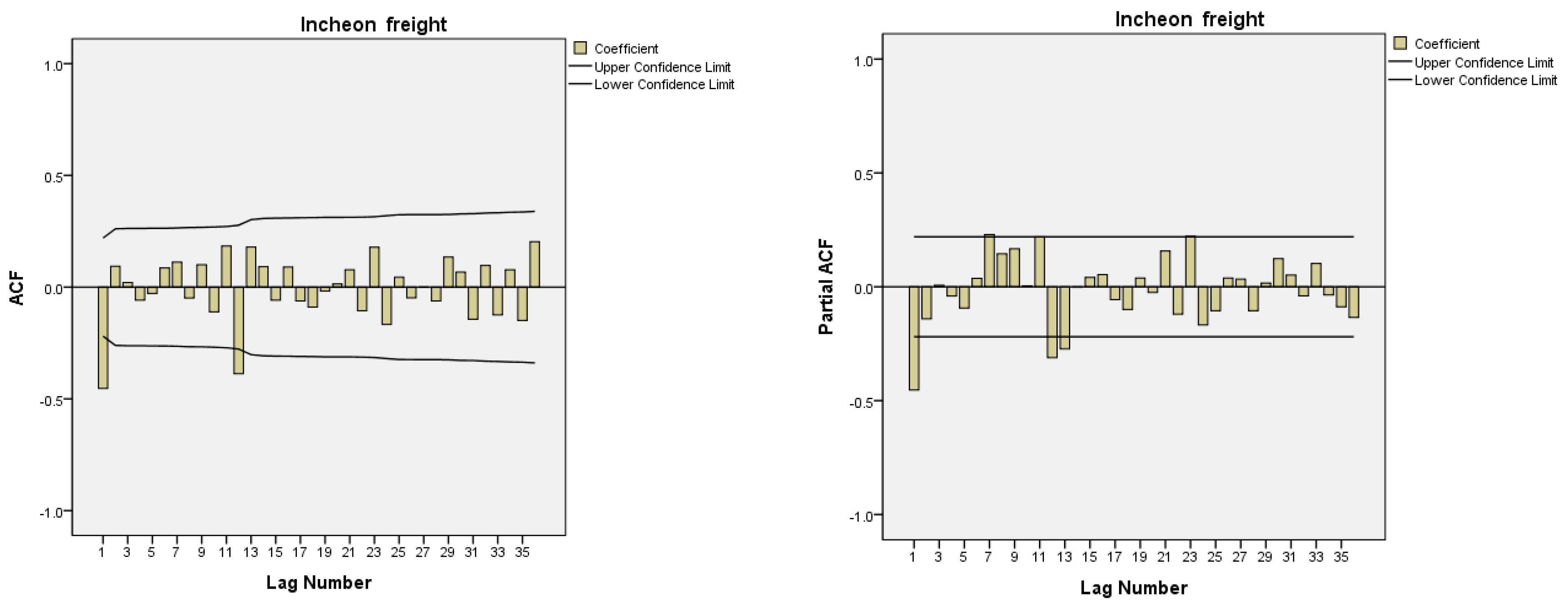
The second step is an identification step in which the correlation between observed values in the time series is measured to temporarily determine autoregressive (AR) elements, p, P, and moving average (MA) elements, q, Q. Correlation is measured by an autocorrelation function (ACF) and a partial autocorrelation function (PACF). The third step is an estimation step which estimates the coefficients of the model selected in the identification step and determines the statistical significance of the estimated parameters. Here, if the estimated parameters are not statistically significant, we must go back to the identification step and temporarily select another ARIMA model. The fourth step is to determine whether the estimated model is statistically appropriate. The fourth step validates the independence of white noise through verification methods such as residual autocorrelation functions, t-test statistics, and chi-squared tests (Ljung–Box Q-tests). The model that matches the verification results is rejected, and the three steps of identification, estimation, and model verification are repeated until a final model is found. Predicted values are obtained based on the model that is finally confirmed.

Lim and McAleer [18] predicted travel demand in Asia–Australia routes through the traditional ARIMA model and the seasonal ARIMA (SARIMA) model. Coshall [19] predicted UK passenger demand for routes connecting 16 main countries to Japan, Canada, the United States, and the Canary Islands. Yüksel [20] predicted the demand for five-star hotel rooms in Ankara, Turkey, based on an ARIMA model.

The seasonal ARIMA (SARIMA) model involves the addition of seasonal terms to the ARIMA model. The process of constructing the model is almost the same as the process of constructing the non-seasonal ARIMA model. In the identification step, two estimated correlation functions are calculated and one or more temporal models are selected by comparing them with two theoretical correlation functions. After estimating the parameters included in the model, the independence of white noise is verified through the residual autocorrelation function. If the null hypothesis is rejected, then another model is temporarily re-identified through the residual autocorrelation function. Unlike non-seasonal time series data, seasonal time series data are correlated with each other at intervals of the length of periodicity (s). By adding seasonality to the general ARIMA model, the SARIMA model is expressed as $\mathrm{ARIMA}\left(\mathrm{p},\mathrm{d},\mathrm{q}\right) {\left(\mathrm{P},\mathrm{D},\mathrm{Q}\right)}_s,$ where $\left(\mathrm{p},\mathrm{d},\mathrm{q}\right)$ represent non-seasonal orders and $\left(\mathrm{P},\mathrm{D},\mathrm{Q}\right)$ represent seasonal orders. This is expressed in the following Equation (1).

$$\begin{array}{l}{\varphi }_p\left(B\right)=\left(1-{\varphi }_{1}B-{\varphi }_2{B}^2-\cdots -{\varphi }_p{B}^p\right)\\ {\mathsf{\Phi }}_P\left(B^s\right)=\left(1-{\mathsf{\Phi }}_s{B}^s-{\mathsf{\Phi }}_{2s}{B}^{2s}-\cdots -{\mathsf{\Phi }}_{Ps}{B}^{Ps}\right)\\ {\nabla }^d={\left(1-B\right)}^d\\ {\nabla }_s^D={\left(1-B^s\right)}^D\\ {\mathsf{\Theta }}_Q(B^s)=\left(1-{\mathsf{\Theta }}_s{B}^s-{\mathsf{\Theta }}_{2s}{B}^{2s}-\cdots -{\mathsf{\Theta }}_{Qs}{B}^{Qs}\right)\\ {\theta }_q\left(B\right)=\left(1-{\theta }_{1}B-{\theta }_2{B}^2-\cdots -{\theta }_q{B}^q\right)\end{array}$$

(1)

Here, ${\varphi }_p\left(B\right)$ is the non-seasonal AR part, ${\mathsf{\Phi }}_P\left(B^s\right)$ is the seasonal AR part, ${\mathsf{\Theta }}_Q(B^s)$ is the seasonal MA part, ${\theta }_q\left(B\right)$ is the non-seasonal MA part, d is the non-seasonal difference order, D is the seasonal difference order, and s is the length of the cycle. The term ${ϵ}_t$ follows a white noise process with a mean of 0 and a variance of ${\sigma }_{ϵ}^2$, assuming that ${ϵ}_t$ and $y_{t-1}, y_{t-2}$, are independent of each other. The term ${\nabla }^d{\nabla }_s^D\widetilde{y_t}$ denotes a normalized time series obtained through non-seasonal and seasonal differential methods to normalize the abnormal time series $\widetilde{\left(y_t\right)}$.

2.2. Delay Time and Delay Cost Analysis

2.2.1. Delay Reduction Model

There are three typical methods for analyzing delay times in flight service due to dangerous weather. First, the delay time may be calculated from the actual departure/arrival time of the flight schedule of any flight corresponding to alarm times announced by the Meteorological Administration. However, there are dozens and dozens of alarms per airport, leading to difficulties in calculation because dozens (hundreds) of aircrafts arrive and depart from various airports during the course of each alarm. The second method is to calculate the actual departure/arrival delay time of a delayed flight from data classified as dangerous aircraft data according to causes of aircraft delay announced by the Korea Airports Corporation (KAC). These data are limited, however, in that they only include cases where the delay time is more than one h. Finally, the delayed model is used as a representative delay analysis model. The method involves a calculation based on time, which affects the number of airports handling departures and arrivals of aircraft in dangerous conditions together with the number of arrivals and departures of aircraft in dangerous conditions. This is an effective method to analyze time-based delay times affecting the number of arrivals/departures and the number of flights under conditions of severe weather [21,22].

This study looks at the basics of the delay reduction model proposed by Evans [23] using the delay reduction model. Delays occur due to several reasons, resulting in aircraft turnaround, industrial actions and operational efficiency. Weather conditions reduce the capacity of an airport terminal for a certain period of time. Fog is main low visibility source, and other main sources are gale, snowfall, rainfall and typhoon. If severe weather lasts for two h, causing aircraft that need to depart from the airport not to depart, as well as situations where landing aircraft cannot land as scheduled, then the resulting “aircraft delay” lasts until grounded aircraft take off and arrive at set destinations [24,25,26].

At this time, if the minimum flight time of the aircraft on the ground is 1 h, then the total delay time is 3 h. The sum of these aircraft delay times can be expressed by the following Equation (2).

$$\mathrm{Z}=0.5T^2\left(D-C_W\right)\left(C_V-C_W\right)/\left(C_V-D\right)$$

(2)

where

• $\mathrm{Z}=\mathrm{Time}\mathrm{of}\mathrm{flight}\mathrm{delays}$(h/month)
• $\mathrm{D}=\mathrm{Number}\mathrm{of}\mathrm{flights}$ (monthly fights/operating time)
• $C_W=\mathrm{Terminal}\mathrm{capacity}\mathrm{on}\mathrm{severe}\mathrm{weather}$ (no. of fights/h)
• $C_V=\mathrm{Terminal}\mathrm{capacity}\mathrm{on}\mathrm{good}\mathrm{weather}$(no. of fights/h)
• $\mathrm{T}=\mathrm{Severe}\mathrm{weather}\mathrm{alert}\mathrm{time}$(h/month)

The term T is the square; thus, if we can reduce alert times for severe weather via more accurate weather forecasts, then delay times of flights will be greatly reduced. The delay reduction model is effective in responding to air traffic management and terminal capacity reduction at airports, and it is advantageous in various studies for its easy calculation of delay times. The work of Allan et al. [27] used a delay reduction model to calculate the economic benefits of flight delays when using the Integrated Terminal Weather System (ITWS) at LaGuardia and John F. Kennedy International airports in New York City. Allan and Evans [28] used this model to calculate operating profits generated when using the ITWS at Atlanta International Airport. Robinson et al. [29] used a delay reduction model to measure delay reduction effects caused by a Route Availability Planning Tool (RAPT) in New York City airports.

2.2.2. Delay Cost Analysis

The cost of flight delays in South Korea is calculated by assigning weights to the frequency of occurrence and setting a representative value in a scenario under the standards of consumer dispute resolution. South Korea’s delay costs are not analyzed according to precise criteria and do not include the opportunity costs of passengers, which is insufficient to produce a clear picture of total economic loss. In general, the method of calculating flight delay costs is mainly based on a method proposed by the European Organization for the Safety of Air Navigation (commonly known as Eurocontrol) that analyzes delay costs by dividing delay costs into three situations [30].

The first situation is a delay situation in which network effects are not reflected. This means that the scenario does not take into account that chain delays are caused by a single original delay. The second situation is a delay situation that reflects network effects. This is a case where chain delays occur due to network effects, such as a delay in a preceding flight affecting a delay in a subsequent flight. The third and final delay situation aims to adjust flight plans by predicting delays. This means that delays are minimized by predicting delays and adjusting flight schedules in advance. Here, delays are categorized as ground delays or in-flight delays, with ground delays defined as delays before and after the landing of flights. In-flight delays refer to delays in route and arrival. In a study on the economic loss of aircraft based on Eurocontrol standards, Cook and Tanner [31] compared the management costs of takeoff delays and in-flight delays. The work of Ferguson et al. [32] used Eurocontrol criteria to analyze delays over a period of time at 19 major airports in the United States by type of aircraft, time of day, and route.

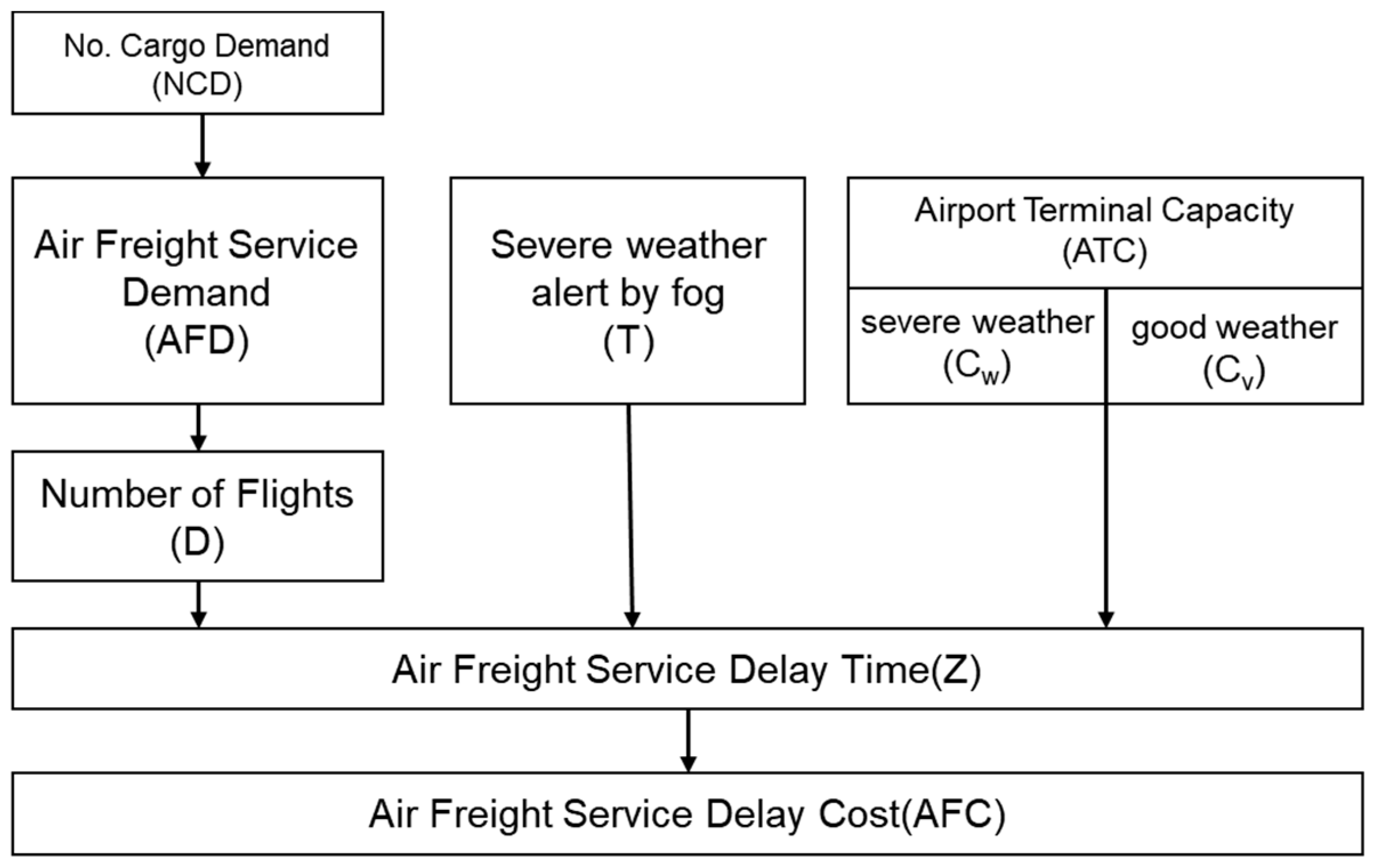
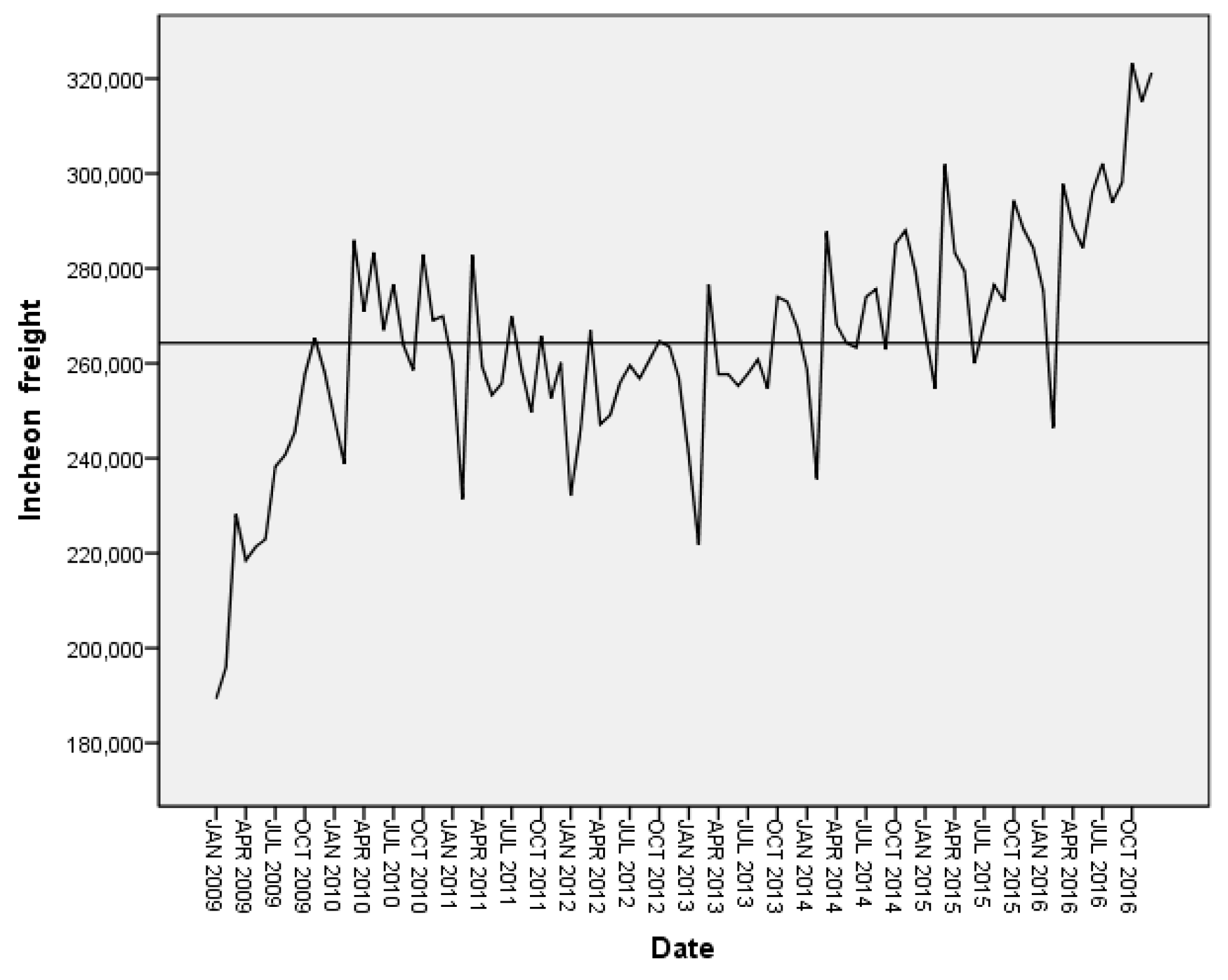
In the current study, demand for air cargo service (cargo throughput) at Incheon International Airport, selected because it has the largest terminal capacity in South Korea, was inputted into the seasonal ARIMA (SARIMA) model for forecasting purposes. We also developed a regression model that predicts the number of flights by regression analysis between air cargo service demand and number of flights. We predicted the delay times of flights by substituting the predicted number of flights and severe weather (i.e., low visibility) alert times into a delay reduction model. This delayed time was calculated according to the delay cost calculation criterion of Eurocontrol, and a model was developed to quantitatively calculate delay costs in air cargo service caused by severe weather conditions.

3. Methodology

3.1. Research Process

The research process to develop a cost forecasting model based on delayed flight service is shown in Figure 1. The first step is forecasting the cargo demand for air cargo service, which is termed air freight demand (AFD). For this purpose, we developed a model to predict cargo demand in aviation operation services using a seasonal ARIMA (SARIMA) model. To ensure the validity of the model, the statistical significance between the predicted values and the observed values was determined through independent sample t-tests.

The second step was forecasting the number of flights (D). A regression model was used to predict the number of flights, and the model was developed based on data predicted in the previous step. For this purpose, observation values of aviation service demand were used as independent variables, and observation values of the number of flights were used as dependent variables. As in the first step, the statistical significance between predicted and observed values was determined through independent sample t-tests to ensure model validity.

The third step was to calculate the air cargo service delay time (Z). At this stage, we developed a model to derive delay times using the delay reduction model established by the Massachusetts Institute of Technology (MIT) Lincoln Laboratory. To ensure the validity of the model, we compared actual delay time data with delay times calculated by the model.

Finally, the delay cost of air freight service (AFC) was calculated based on delay cost calculation standards of Eurocontrol. Analysis herein involved three domestic airports with the largest demand for air cargo service at the airport complex of Incheon International Airport (ICN) in South Korea.

4. Analysis Results

4.1. Aviation Service Demand Forecasting Model

4.1.1. Stationarity Verification

This study focused on developing a cost forecasting model for air cargo service delay due to low visibility. Data used in this study were time series data provided by Incheon International Airport Corporation, with monthly data on cargo throughput at Incheon International Airport from January 2009 to December 2016. Four hundred and fifty-seven (4.61%) of 9908 flights in 2017 and 470 (5.24%) of 8972 flights in 2018 were delayed due to low visibility by fog at Incheon International Airport [16].

Before building the forecasting model, we used time series charts and autocorrelation functions to check for the presence of trends and seasonality in time series data. Figure 2 shows the time series chart of cargo throughput at Incheon International Airport. We verified that patterns with a one-year cycle were repeated and that cargo throughput increased over time. It was necessary to establish these data as a normal time series because it was a seasonal anomalous time series which combined general time differences and seasonal time differences. Statistical software SPSS 21.0 (IBM Inc, Chicago, USA) was used for data analysis herein. Figure 2 shows the cargo throughput at Incheon airport form January 2009 to December 2016.

To ensure stationarity in these time series data, the first non-seasonal difference was applied, with results as shown in Figure 3; Figure 4. Using the autocorrelation function (ACF), a pattern that was repeated after the first non-seasonal difference was identified. This means that there was a seasonal pattern in these data. Therefore, a seasonal difference was additionally required.

Figure 5 is a time series chart that shows stationarity with the non-seasonal first difference and seasonal first difference in Incheon Airport data. In this chart, the cargo throughput at Incheon International Airport fluctuates around an average. This implies that the trend and seasonality have been removed and transformed to normal time series data. Accordingly, model estimation was performed based on this observation.

4.1.2. Model Estimation

Based on the time series data with stationarity, we estimated the model by using an ACF and a partial autocorrelation function (PACF) results for non-seasonal and seasonal first differences. Based on the results shown in Figure 6, two models of $\mathrm{ARIMA}\left(0,1,1\right){\left(1,1,0\right)}_{12}$ and $\mathrm{ARIMA}\left(1,1,0\right){\left(1,1,0\right)}_{12}$ were considered and were found to be statistically insignificant. The constant term was excluded from the model. In order to objectively evaluate the model, the normalized Bayesian information criterion (BIC) based on the Bayesian method was used.

Table 1. Model statistics.

Model	$\mathbf{Stationary}{\mathit{R}}^2$	Ljung–Box Q
		Statistics	DF	p-value
$\mathrm{ARIMA}\left(0,1,1\right){\left(1,1,0\right)}_{12}$	0.335	24.670	16	0.076
$\mathrm{ARIMA}\left(1,1,0\right){\left(1,1,0\right)}_{12}$	0.358	22.974	16	0.114

shows the BIC values for validation of selected models. Among them, the $\mathrm{ARIMA}\left(1,1,0\right){\left(1,1,0\right)}_{12}$ model with a small BIC value of 18,616 was identified as the optimal model.

Table 2. Model estimation.

Model		Estimate	S.E.	t-Value	p-Value
$\mathrm{ARIMA}\left(0,1,1\right){\left(1,1,0\right)}_{12}$	MA, Difference 1	0.436	0.103	4.245	0.000
	AR, Seasonal Difference 1	−0.467	0.108	−4.331	0.000
$\mathrm{ARIMA}\left(1,1,0\right){\left(1,1,0\right)}_{12}$	AR, Difference 1	−0.500	0.097	−5.163	0.000
	AR, Seasonal Difference 1	−0.505	0.107	−4.735	0.000

;

Table 3. Model fit.

Fit Statistics	$\mathbf{ARIMA} \left(0,1,1\right) {\left(1,1,0\right)}_{12}$	$\mathbf{ARIMA} \left(1,1,0\right) {\left(1,1,0\right)}_{12}$
Stationary $R^2$	0.335	0.358
$R^2$	0.722	0.731
RMSE	10,360.267	10,180.321
MAPE	3.088	3.153
MaxAPE	11.103	10.989
MAE	8136.959	8331.520
MaxAE	27,181.964	25,428.234
Normalized BIC	18.651	18.616

show model estimates and fit with estimated model parameters. The estimated parameters of the $\mathrm{ARIMA}\left(1,1,0\right){\left(1,1,0\right)}_{12}$ model were statistically significant.

Based on the above results, the final forecasting Equation (3) used to predict cargo demand at Incheon International Airport can be derived.

$$\left(1+0.500B\right)\left(1+0.505B^{12}\right)\left(1-B\right)\left(1-B^{12}\right)\widetilde{y_t}={ϵ}_t$$

(3)

The $\mathrm{ARIMA}\left(1,1,0\right){\left(1,1,0\right)}_{12}$ showed an explanatory power of about 88.6%, and the significance probability was greater than the significance level of 0.05. Therefore, it is confirmed that white noise existed independently and the $\mathrm{ARIMA}\left(1,1,0\right){\left(1,1,0\right)}_{12}$ was suitable as a prediction model. Based on the cargo demand forecasting model developed in this study for Incheon International Airport, predicted values from January 2017 to December 2018 were derived. As shown in

Table 4. Forecasting results of cargo demand at Incheon International Airport.

Time	Observed Values	Expected Values	Error Rate
Jan-17	299,986	303,021	−1.01%
Feb-17	283,220	284,485	−0.45%
Mar-17	329,998	330,020	−0.01%
Apr-17	313,415	316,469	−0.97%
May-17	304,547	309,758	−1.71%
Jun-17	309,066	301,638	2.40%
Jul-17	319,864	310,979	2.78%
Aug-17	319,227	317,540	0.53%
Sep-17	327,607	319,142	2.58%
Oct-17	320,731	345,728	−7.79%
Nov-17	339,410	328,145	3.32%
Dec-17	339,180	326,296	3.80%
Jan-18	320,168	324,061	−1.22%
Feb-18	283,739	298,485	−5.20%
Mar-18	341,633	338,919	0.79%
Apr-18	323,687	323,832	−0.04%
May-18	322,925	319,041	1.20%
Jun-18	320,663	327,464	−2.12%
Jul-18	331,671	333,525	−0.56%
Aug-18	329,016	324,915	1.25%
Sep-18	329,946	333,431	−1.06%
Oct-18	344,526	341,677	0.83%
Nov-18	339,216	346,035	−2.01%
Dec-18	330,741	346,576	−4.79%

, the actual values of Incheon International Airport from January 2007 to December 2018 were similar to those predicted using $\mathrm{ARIMA}\left(1,1,0\right){\left(1,1,0\right)}_{12}$.

4.2. Forecasting Model for Number of Flights

We developed a regression model that forecasts the number of flights based on the demand for air cargo service (cargo throughput). The independent variable was the cargo throughput, the dependent variable was the number of flights, and data from January 2009 to December 2016 were used in Incheon International Airport Corporation. Time series data that change with time may not follow a normal distribution, so logarithm and regression analysis may be performed if necessary. For this analysis, we assumed the aircraft type to be freighter of the airliner and freighter. Additionally, cargo type was assumed to be air cargo. The size of the aircraft was not included in the assumption. The number of delays due to A/C (Air Craft) connection was also excluded from the total number of delayed units. Regression analysis results for Incheon International Airport are shown in

Table 5. Regression analysis for forecasting the number of flights.

Model	Unstandardized Coefficients		Standardized Coefficients	t (p)
	B	S.E.	$\mathsf{\beta }$
(Constant)	−9.281	1.235		−7.515 ***
log_cargo	1.544	0.099	0.822	15.654 ***

F = 245.062 ***; R² = 0.675; Adjusted R² = 0.672; p < 0.01.

.

Independent sampling t-tests were performed on the observed values of the number of airline flights and the predicted values calculated by the regression model. According to the results, there was no statistically significant difference between the predicted values and the observed values (p > 0.05). Therefore, the regression model for Incheon International Airport is reasonable for analyzing forecast values. The estimated and observed values from January 2017 to December 2018, which were derived from the proposed regression model for Incheon International Airport and the predicted demand for air cargo services, are shown in

Table 6. Forecasting results of number of flights at Incheon International Airport.

Time	Observed Values	Expected Values	Error Rate
Jan-17	30,340	27,084	10.7%
Feb-17	27,478	24,569	10.6%
Mar-17	29,336	30,899	−5.3%
Apr-17	28,187	28,962	−2.7%
May-17	29,440	28,019	4.8%
Jun-17	28,910	26,893	7.0%
Jul-17	31,175	28,190	9.6%
Aug-17	31,893	29,113	8.7%
Sep-17	30,117	29,340	2.6%
Oct-17	31,396	33,199	−5.7%
Nov-17	30,127	30,628	−1.7%
Dec-17	31,896	30,362	4.8%
Jan-18	33,171	30,041	9.4%
Feb-18	29,902	26,460	11.5%
Mar-18	32,383	32,194	0.6%
Apr-18	31,200	30,009	3.8%
May-18	32,089	29,326	8.6%
Jun-18	31,641	30,530	3.5%
Jul-18	33,029	31,407	4.9%
Aug-18	33,804	30,164	10.8%
Sep-18	31,721	31,393	1.0%
Oct-18	33,081	32,600	1.5%
Nov-18	32,144	33,244	−3.4%
Dec-18	33,568	33,324	0.7%

. The average error rate of the estimated number of flights at Incheon International Airport was 4%.

4.3. Delay Time and Cost Analysis Model

We calculated delay time in aviation services by using a delay reduction model. Based on the cost calculation standards of Eurocontrol (100.65 €/min), delay costs were calculated via multiplication of values with delay times [29]. The currency standard of Eurocontrol is the euro (€). The results from January 2017 to December 2018 are shown in

Table 7. Forecasting result of delay time and cost by low visibility at Incheon International Airport.

Time	Delay Time (min)	Delay Cost ($)
Jan-17	-	-
Feb-17	-	-
Mar-17	367	41,730.13
Apr-17	4318	490,618.65
May-17	-	-
Jun-17	8378	952,043.18
Jul-17	-	-
Aug-17	-	-
Sep-17	-	-
Oct-17	7755	881,215.00
Nov-17	-
Dec-17	1407	159,913.25
Total	22,225	2,525,520.20
Jan-18	-	-
Feb-18	-	-
Mar-18	76,772	9,120,660.50
Apr-18	525	62,395.62
May-18	-	-
Jun-18	449	53,382.04
Jul-18	11,457	1,361,047.64
Aug-18	-	-
Sep-18	-	-
Oct-18	-	-
Nov-18	-	-
Dec-18	-	-
Total	89,203	10,597,485.80

. The total delay time in aviation services in 2017 due to low visibility at Incheon International Airport was estimated to have been 22,225 min (370.42 h), and the total delay costs resulting from this delay time was estimated to be around $2.53 million. The total delay time in 2018 was estimated to have been 89,203 min (1486.72 h), with total estimated delay costs around $10.60 million.

5. Conclusions

In recent years, consumer demand for rapid delivery has grown, and the development of comprehensive logistics has led to an increase in air cargo transportation. In the past, the cost of air cargo was relatively high, mainly operated by a small sector of transportation centered on IT and high-value products. Today, however, the connection between air transportation and land transportation has been enhanced to improve the speed and timeliness of cargo transportation.

In an environment where supply chain globalization has expanded and the importance of air cargo transportation has increased, weather factors are very important factors affecting operating costs. This study selected low visibility due to fog as a representative factor affecting air cargo transportation delay for analysis. The purpose of this study was to suggest implications for the cost aspect of air cargo operation by predicting delay costs based on delay times caused by low visibility.

In airports, multitudinous delays in flight service are due to many types of dangerous conditions for aviation operation. This study developed a model that quantitatively calculates and predicts delay costs in air navigation service at a South Korean airport (i.e., the Incheon airport complex due to low visibility). In this study, we estimated and forecasted delay costs based on weather factors in order to make strategic decisions about operational costs to improve air cargo service. The model for the prediction of delay costs developed herein can be further utilized to quantitatively estimate economic loss due to delays caused by factors other than low visibility. March of 2018 had a heavy influence on total delay of 2018 and therefore on the cost of delay. This value was very exceptionally high, but it was not a persistent situation of low visibility. Incheon International Airport is located in the western part of Korea. In March 2018, the Meteorological Administration and Incheon International Airport (KICA) confirmed that a number of low-visibility alerts of Incheon were issued due to the heavy fog and fine dust caused by the west coast, resulting in high delay time. There are several ways to improve the service delay in an air transportation. One way is to properly utilize the ILS (instrumental landing system) category possessed by the airport, which obviously influences the total amount of delay. The ILS is the most popular landing aid in the world. It is a distance-angled support system for landing in reduced visibility, and its task is the safe conduct of the aircraft from the prescribed course landing on the approach path. Additionally, a target operation under low visibility conditions may be allowed, depending on the lowest figure among airport ILS, aircraft onboard equipment and pilot certification.

In conclusion, delay costs caused by low visibility have been shown to increase, depending on air cargo service. Thus, service delays due to low visibility should be improved. Our proposed model estimates economic losses for strategic decisions aiming to improve air cargo service. This model is applicable to other similar settings as well.

References

1. IATA. Air Freight Market Analysis; IATA: Montreal, QC, Canada, 2019. [Google Scholar]
2. Alkaabi, K.A.; Debbage, K.G. The geography of air freight: Connections to U.S. metropolitan economies. J. Transp. Geogr. 2011, 19, 1517–1529. [Google Scholar] [CrossRef]
3. Baker, D.A.; Crompton, J.L. Quality, satisfaction and behavioral intentions. Ann. Tour. Res. 2000, 27, 785–804. [Google Scholar] [CrossRef]
4. Hong, S.; Zhang, A. An efficiency study of airlines and air cargo/passenger divisions: A DEA approach. World Rev. Intermodal Transp. Res. 2010, 3, 137–149. [Google Scholar] [CrossRef]
5. Becker, B.; Dill, N. Managing the complexity of air cargo revenue management. J. Revenue Pricing Manag. 2007, 6, 175–187. [Google Scholar] [CrossRef]
6. Yang, T.H. Stochastic air freight hub location and flight routes planning. Appl. Math. Model. 2009, 33, 4424–4430. [Google Scholar] [CrossRef]
7. Kasilingam, R. Air cargo revenue management: Characteristics and complexities. Eur. J. Oper. Res. 1997, 96, 36–44. [Google Scholar] [CrossRef]
8. Suryani, E.; Chou, S.Y.; Chen, C.H. Dynamic simulation model of air cargo demand forecast and terminal capacity planning. Simul. Model. Pr. Theory 2012, 28, 27–41. [Google Scholar] [CrossRef]
9. Rondinelli, D.; Berry, M. Multimodal transportation, logistics, and the environment: Managing interactions in a global economy. Eur. Manag. J. 2000, 18, 398–410. [Google Scholar] [CrossRef]
10. Chang, Y.H.; Yeh, C.H.; Wang, S.Y. A survey and optimization-based evaluation of development strategies for the air cargo industry. Int. J. Prod. Econ. 2007, 106, 550–562. [Google Scholar] [CrossRef]
11. Alexander, D.W.; Merkert, R. Challenges to domestic air freight in Australia: Evaluating air traffic markets with gravity modelling. J. Air Transp. Manag. 2017, 61, 41–52. [Google Scholar] [CrossRef]
12. Boonekamp, T.; Burghouwt, G. Measuring connectivity in the air freight industry. J. Air Transp. Manag. 2017, 61, 81–94. [Google Scholar] [CrossRef]
13. Hong, S.-J.; Randall, W.; Han, K.; Malhan, A.S. Estimation viability of dedicated freighter aircraft of combination carriers: A data envelopment and principal component analysis. Int. J. Prod. Econ. 2018, 202, 12–20. [Google Scholar] [CrossRef]
14. Lange, A. Does cargo matter? The impact of air cargo operations on departure on-time performance for combination carriers. Transp. Res. Part. A: Policy Pr. 2019, 119, 214–223. [Google Scholar] [CrossRef]
15. Bureau of Transportation Statistics. U.S. Airport Delays by Cause; US Department of Transportation: Washington, DC, USA, 2017.
16. Incheon International Airport Corporation (IIAC). Incheon International Airport Statistics; Airport Research Center: Incheon, South Korea, 2019. [Google Scholar]
17. Box, G.E.P.; Jenkins, G. Time Series Analysis, Forecasting and Control; Holden-Day: San Francisco, CA, USA, 1970. [Google Scholar]
18. Lim, C.; McAleer, M. Time series forecasts of international travel demand for Australia. Tour. Manag. 2002, 23, 389–396. [Google Scholar] [CrossRef]
19. Coshall, J. Time Series Analyses of UK Outbound Travel by Air. J. Travel Res. 2006, 44, 335–347. [Google Scholar] [CrossRef]
20. Yuksel, S. An integrated forecasting approach to hotel demand. Math. Comput. Model. 2007, 46, 1063–1070. [Google Scholar] [CrossRef]
21. National Research Council, National Aviation Weather Services Committee. Aviation Weather Services: A Call for Federal Leadership and Action; National Academies Press: Washington, DC, USA, 1995. [Google Scholar]
22. Robinson, M.; Evans, J.; Crowe, B.; Klingle-Wilson, D.; Allan, S. Corridor Integrated Weather System Operational Benefits 2002–2003: Initial Estimates of Convective Weather Delay Reduction; MIT Lincoln Laboratory: Lexington, MA, USA, 2004. [Google Scholar]
23. Evans, J. Measuring the Economic Value of Aviation Meteorological Products. In Proceedings of the 14th Conference on Weather Analysis and Forecasting, Dallas, TX, USA, 2–6 January 1995. [Google Scholar]
24. Malandri, C.; Mantecchini, L.; Reis, V. Aircraft turnaround and industrial actions: How ground handlers’ strikes affect airport airside operational efficiency. J. Air Transp. Manag. 2019, 78, 23–32. [Google Scholar] [CrossRef]
25. Herman, G.R.; Schumacher, R.S. Using Reforecasts to Improve Forecasting of Fog and Visibility for Aviation. Weather. Forecast. 2016, 31, 467–482. [Google Scholar] [CrossRef]
26. Wang, F.; Zhuo, X.; Niu, B. Strategic entry to regional air cargo market under joint competition of demand and promised delivery time. Transp. Res. Part. B: Methodol. 2017, 104, 317–336. [Google Scholar] [CrossRef]
27. Allan, S.S.; Gaddy, S.G.; Evans, J.E. Delay Causality and Reduction at the New York City Airports Using Terminal Weather Information Systems; MIT Lincoln Laboratory: Lexington, MA, USA, 2001. [Google Scholar]
28. Allan, S.; Evans, J. Operational Benefits of the Integrated Terminal Weather System (ITWS) at Atlanta; MIT Lincoln Laboratory: Lexington, MA, USA, 2005. [Google Scholar]
29. Robinson, M.; DeLaura, R.; Evans, J.; McGettigan, S. Operational Usage of the Route Availability Planning Tool During the 2007 Convective Weather Season; MIT Lincoln Laboratory: Lexington, MA, USA, 2008. [Google Scholar]
30. EuroControl. Standard Input for EUROCONTROL Cost-Benefit Analyses; EuroControl: Brussels, Belgium, 2015. [Google Scholar]
31. Cook, A.J.; Tanner, G. The Challenge of Managing Airline Delay Costs. In Proceedings of the Conference on Air Traffic Management Economics, Belgrade, Serbia, 10–11 September 2009. [Google Scholar]
32. Ferguson, J.; Kara, A.Q.; Hoffman, K.; Sherry, L. Estimating domestic US airline cost of delay based on European model. Transp. Res. C: Emerg. Technol. 2013, 33, 311–323. [Google Scholar] [CrossRef]
Figure 1. Proposed cost forecasting model framework for delays due to low visibility.
Sustainability 11 04390 g001
Figure 2. Cargo throughput at Incheon airport.
Sustainability 11 04390 g002
Figure 3. First non-seasonal difference in Incheon airport cargo throughput.
Sustainability 11 04390 g003
Figure 4. Autocorrelation function (ACF) results of the first non-seasonal difference.
Sustainability 11 04390 g004
Figure 5. Non-seasonal and seasonal first differences in Incheon cargo throughput.
Sustainability 11 04390 g005
Figure 6. ACF and partial autocorrelation function (PACF) results of non-seasonal and seasonal first differences.
Sustainability 11 04390 g006