Exploring the Relationship between Urban Vitality and Street Centrality Based on Social Network Review Data in Wuhan, China

Abstract

This study investigates the association between urban vitality and street centrality in Wuhan, China. Urban vitality was measured with social network review data. Street centrality was evaluated in terms of closeness, straightness, and betweenness in walking and driving mode. We constructed a square mesh to convert datasets of street centrality (segments) and urban vitality (points) into one unit for analysis. Geospatial visualization, a chi-square test, and correlation analysis were first employed to obtain an initial understanding of the spatial coupling relationship between urban vitality and street centrality. Then spatial regression models were applied to evaluate the significances and directions of the influences of street centrality on urban vitality. A geographical detector technique was utilized to further evaluate the magnitudes of these influences. The results suggest that street centrality plays an important role in shaping the spatial organization of urban vitality, and various street centralities presented marked differences in their association with urban vitality. More specifically, when considering street centrality in walking mode, betweenness affected urban vitality the most, followed by closeness and straightness. When considering street centrality in driving mode, straightness had the greatest influence on urban vitality, followed by closeness and betweenness.

1. Introduction

1.1. Urban Vitality

Urbanization processes in most Chinese cities share common characteristics, such as rapid and poor-quality sprawling, while vitality has commonly been underappreciated by urban planners and designers [1]. With a rise in income and enrichment in material wealth, people have begun to reconsider previous city development patterns and have called for creating vibrant and energetic urban space [2]. By providing viable places for sociability, connections, and involvement in multiple activities, the vibrant urban environment is beneficial to the economy and people’s social and economic lives [3,4].

Although the benefit of vitality has been recognized and extensive research has been done on urban vitality, it is difficult to capture the rich meaning of urban vitality in a specific definition. Jacobs [5] described urban vibrancy as the intensity of pedestrian activity on city streets, and well-organized dense functional spaces could generate adequate interactions and activities for creating vibrancy. Based on Jacobs’s view, Montgomery [6] promoted viable street life, which includes pedestrian flows on the street and the presence of small-scale business activities. Urban vitality has also been regarded as the raw power and energy within a city [7], human activities in different places [8], and essential elements for achieving an urban quality of life [9].

Various measurements have been proposed to evaluate urban vitality. Wang and Guldmann [10] used a combination of population and employment density to measure urban vitality. Braun and Malizia [11] created an urban vibrancy index by compositing compactness, density, regional and local connectivity, destination accessibility, land use mix, and social diversity. Other measurements of urban vitality have included nighttime light data [12], population census data [13], and land price [14]. However, these measurements have some flaws: traditional data acquisition methods such as surveying and interviewing are time-consuming and laborious, and land use and nighttime light data are usually obtained on a regional scale, so they cannot capture the local spatial variation of urban vitality.

In recent studies, geotagged food facilities have been frequently used to estimate urban vitality [1,15,16]. Research has demonstrated that food facility is an essential component of urban life, and it can effectively indicate the attractiveness of a location [17]. The validity of using food facilities to proxy urban vitality can be explained from three perspectives. First, the success of a business depends to a great extent on location [18]. Central place theory indicates that stores tend to locate in accessible places that attract dense and diverse streams of people, and these crowds are directly related to the survival and development of the catering business [19,20]. Therefore, the spatial organization of food facilities can reflect the variation of human activity to a great extent. Second, the locations of large-sized buildings such as supermarkets and entertainment centers are usually selected based on market and symbolic reasons, which makes them unsuitable for measuring urban vitality. The building sizes of food facilities in Chinese cities, however, are usually not large enough to (re)shape the neighboring architecture configuration. Therefore, food facilities can better reflect existing urban vitality [1]. Finally, the spatial organization of food facilities is formed by the common effect of business owners and the public, who are all self-motivated people. Food facilities, therefore, are suitable as “indicator businesses” for lively urban areas.

Emerging sources from social network data provide us a new lens for understanding the vibrancy of a city. Social network data are accessible and convenient for gathering crucial information in a short time [21]: studies have confirmed that promising results could be generated by taking advantage of social network data, which are based on a massive number of users [22,23]. Some popular websites such as Yelp (founded in the U.S.) and Dianping (founded in China) provide platforms for people to publish their comments on commercial facilities. The number of reviews on food facilities are usually far more than on other commercial facilities. This is probably because people are more willing to comment on food facilities after they visit these places [15]. Compared to food facilities with few reviews, food facilities with more reviews tend to attract more customers, and human activities in these locations are hence more intense. The level of activity intensity can be used as a proxy for urban vibrancy [24].

In line with previous studies, urban vitality in the context of this study indicates the concentration of people. The total number of social network reviews of food facilities in a location are used as a proxy for urban vibrancy.

1.2. Relationship between Urban Vitality and Street Centrality

Immaterial city life is significantly affected by physical urban space, i.e., the built environment [25]. Urban vitality, in this regard, has been widely recognized to be closely related to urban form [1,26]. Different regions have different levels of vitality due to different urban structures. Therefore, it is necessary to explore the relationship between city form and urban vitality to better understand how the built environment affects human activity.

A road network serves as the “skeleton” of a city because it reveals where most of the crucial components of a city are located, and movements of people are largely constrained along streets as they travel from one place to another [27]. Street centrality is a valid measurement of spatial accessibility and location advantage in a city [28]. A central location can be accessed easily from other locations by people living or working in the city. Additionally, many studies have demonstrated the significant role of street centrality in shaping the intraurban variation in vitality. For instance, Cui et al. [29] investigated karaoke bars’ location patterns in Nanjing, China, and found that street network centrality exerted a crucial impact on the distribution of karaoke bars. A study of the influence of street network configuration on walking volume in Seoul, Korea, demonstrated that locations with high accessibility had high walking volumes [30]. An experimental study of the associations between street centrality and population (residential) and employment (business) densities in Baton Rouge, Louisiana, revealed that they were highly associated with each other in space [31]. Many other studies have also confirmed the significant role of street centrality in facilitating urban vitality [1,32,33,34].

How to mathematically characterize complex street network structures is the premise of studying the relationship between street networks and related geographic events. Porta et al. [35] proposed a multiple centrality assessment (MCA) model to measure location advantages in a city. The MCA is composed of three network-based centrality indices, i.e., closeness, straightness, and betweenness. Three indices evaluate street centrality from different perspectives. Closeness measures the degree to which a location is close to other locations along the shortest routes in the street network. Straightness indicates the extent to which a location is accessible via straight paths to other locations. Betweenness evaluates the frequency of a location being traversed along the shortest paths connecting other locations. Compared to single-index measurements such as street density [36], street connectivity [37], and gravity-based accessibility [38], the MCA provides a more comprehensive and profound interpretation of street configuration. As a widely used model, the validity of the MCA has been verified thoroughly by previous studies. For example, Rui and Ban [28] demonstrated that three street centrality indices provided by the MCA model could efficiently capture the spatial distribution features of urban activities: the MCA is, therefore, useful in characterizing urban structure. Based on the MCA model, Wang et al. [34] analyzed the relationships between densities of various retail stores and street centralities in Changchun, China. The resulting strong associations confirmed the effectiveness of the MCA in revealing the inter-relationship between street networks and retail stores in an urban environment. Another study in Guangzhou, China, also demonstrated the significant role of street centrality in affecting the spatial distribution of retail stores. Additionally, different types of stores have different centrality orientations [33]. Street centrality is the core of the space syntax theory through the concepts of “visibility” and “integration” [39]. In addition, the MCA model shares with space syntax essential values that refer to the structural interpretation of urban spaces, while offering a new and deeply alternative technical perspective [40].

Many studies have explored the association between urban vitality and street centrality. However, these research works still have had some limitations. First, urban vitality is usually proxied by point of interest (POI) data such as retail and food stores. The attractiveness differences between stores are ignored, as each point feature is treated with equal importance [33,34]. Second, most studies used bivariate linear correlation analysis methods such as the Pearson correlation coefficient to examine the relationship between street centrality and urban vitality [31,40]. Many other important influences of urban vitality are omitted, making it impossible to single out the effect of street centrality. Third, people may perceive street layouts differently in different travel modes (e.g., walking and driving). However, most studies so far have measured street centrality without distinguishing travel modes. Finally, urban vitality is a type of typical geographic event that is autocorrelated in space [41]. Very little research has paid attention to this effect.

The main contributions of this study are as follows: (1) A rich set of social network review data on food facilities was collected to proxy urban vitality, in which each facility was weighted by its attractiveness (i.e., number of reviews); and (2) the MCA model was utilized to measure street centrality from three perspectives (closeness, straightness, and betweenness). Notably, different network distance thresholds were used to differentiate street centrality in walking and driving mode and subsequently (3) explore the association between urban vitality and street centrality in walking and driving mode. More specifically, we first created a fine square mesh to convert urban vitality (at point) and street centrality (at segment) datasets into one analysis unit, based on which an exploratory spatial coupling analysis and a correlation analysis were conducted to obtain an initial understanding of the urban vitality–street centrality relationship. Considering the spatial autocorrelation effect, we employed spatial regression models to obtain a robust estimation of the effect of street centrality on urban vitality. To single out the influences of street vitality, a set of control variables was collected and included in these models. Finally, a geographical detector technique was used to evaluate the magnitudes of the effects of these variables. This study focused on Wuhan, the largest city in Central China. We hope to provide useful information for planning and design practice as well as a reference for future research.

2. Materials and Methods

2.1. Study Area and Data Preparation

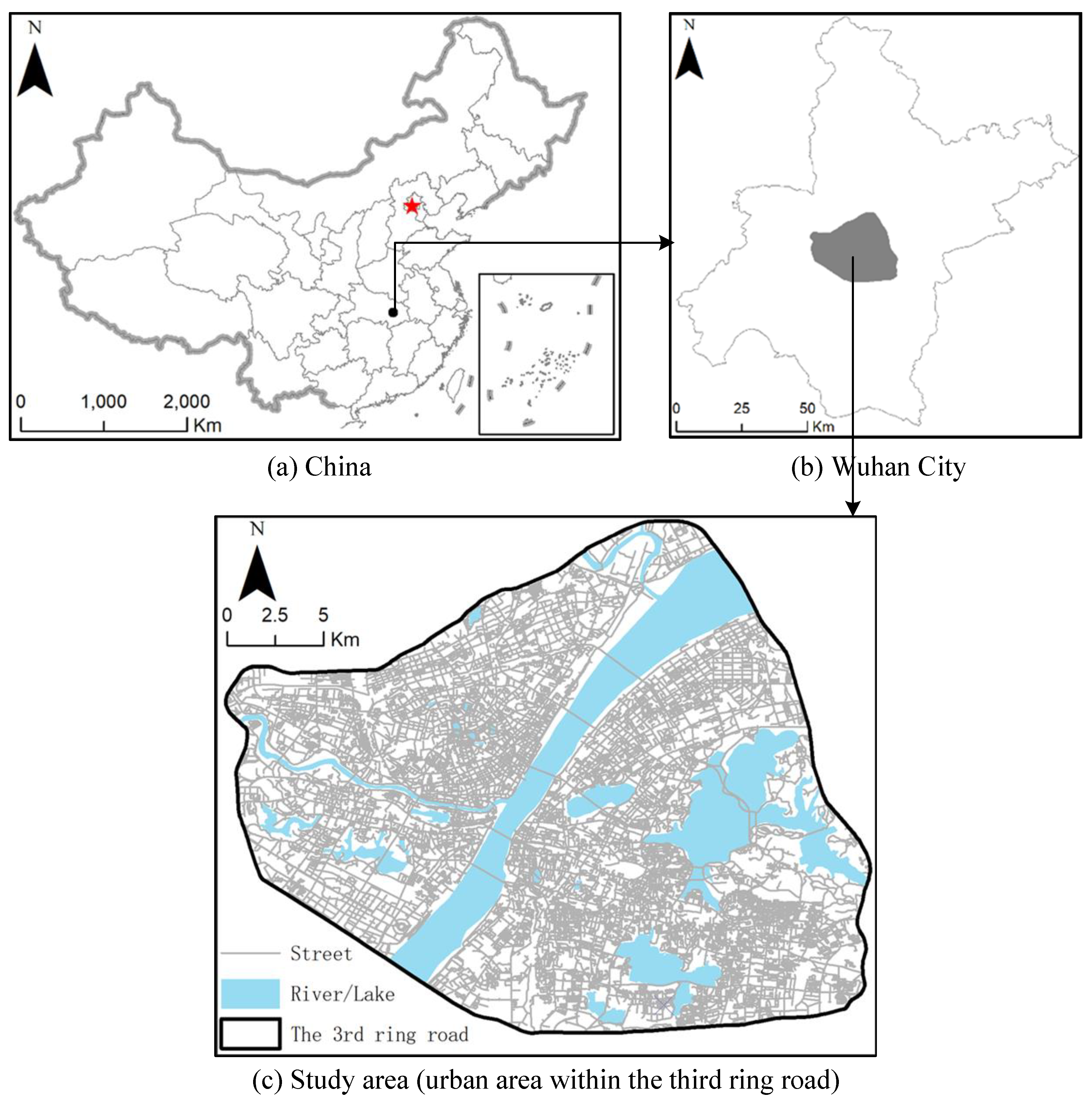
2.1.1. Study Area

Wuhan (29°58′–31°22′ N, 113°41′–115°05′ E), as the capital of Hubei Province, is the largest city in Central China. It covers an area of 8569 km² and had a population of 10.89 million in 2017. After four decades of steady economic growth since reforms and the opening up of China, Wuhan’s GDP reached 1341 billion RMB in 2017, which ranked eighth in China [42]. Wuhan’s per capita disposable income was 38,642 RMB in 2017, which was 48.77% higher than the average level in China (25,974 RMB). As the central government advocated for “building an ecological civilization” in 2007, the economic development of Wuhan is transforming from a high reliance on traditional industries such as the steel and automobile industries to an emphasis on environmentally friendly industries such as catering, retail, and the tourism industry. The proportion of tertiary industry to GDP in Wuhan rose from 49.9% in 2007 to 53.3% in 2017. The emerging catering, tourism, and financial industries have created abundant jobs and have attracted people from nearby cities to work and live here. In 2017, the migrant population was 2.36 million in Wuhan, which accounted for 21.67% of the total population [42]. Among these migrant people, 1.2 million were college students, and this number was first in the world. Additionally, Wuhan was visited by more than 257.14 million domestic travelers and 2.5 million foreign travelers in 2017. A large number of tourists, together with young college students and local residents in this city, have a strong demand for consumption, entertainment, and travel. All of these economic and demographic factors promote the vitality of Wuhan.

As presented in Figure 1, this study focuses on the region within the Third Ring Road. We chose this region because it is the most urbanized part of Wuhan and has a large size of 525 km².

2.1.2. Social Network Review Data

Dianping (http://www.dianping.com) is the largest independent third-party consumer reviews website in China. Similarly to Yelp, it provides a platform for users to publish business information and consumer reviews on commercial facilities [15]. On the Dianping website, food facilities receive far more reviews than other commercial facilities. Through the web crawler technique, we obtained 21,107 records of food facilities in the study area in 2017. Each record had these attributes: shop ID, shop name, address, coordinates, and the number of reviews. Each review represented a customer trip. Therefore, a facility with more reviews could attract more customers and contribute more to urban vitality. This study utilized the number of reviews of food facilities as a proxy for urban vitality. Previous studies have used the number of facilities to measure urban vitality. This was deficient, as they failed to distinguish facilities with high vitality from facilities with low vitality.

2.1.3. Centrality Assessment of Street Network

This study uses the primal approach to represent a road network: road intersections are expressed as nodes, and road segments are expressed as edges with lengths that connect nodes [43]. The primal approach can intuitively reveal the real road network and preserve its metric nature. The number of nodes (street intersections) and edges (street segments) of the street network in the study area was 17,903 and 25,096, respectively.

Three indices provided by the MCA model were used to comprehensively measure street centrality: closeness, straightness, and betweenness.

Closeness C^C evaluates how close a street segment is to other segments along the shortest paths [44]. C^C of segment i is formulated as

$$C_i^C=\frac{N-1}{{{\displaystyle \sum }}_{j=1,j\ne i}^N{d}_{ij}}\left(d_{ij}\le b\right),$$

(1)

where $C_i^C$ is the closeness of segment i, $d_{ij}$ is the minimum network distance between the centroid of segment i and the centroid of segment j, N is the total number of segments, and b is a network distance threshold. A segment with a large closeness has high accessibility or proximity.

Straightness C^S measures the difference between the lengths of the shortest routes from a segment to other segments and the lengths of virtual straight lines connecting them. It is defined as

$$C_i^S=\frac{1}{N-1}{{\displaystyle \sum }}_{j=1,j\ne i}^N\frac{d_{ij}^{Eucl}}{d_{ij}} \left(d_{ij}\le b\right),$$

(2)

where $d_{ij}^{Eucl}$ means the Euclidean distance between the centroid of segment i and the centroid of segment j. A segment with high straightness has high efficiency or legibility [45].

Betweenness C^B indicates how frequently a segment is traversed by the shortest paths between any two segments. It is calculated as,

$$C_i^B=\frac{1}{\left(N-1\right)\left(N-2\right)}{{\displaystyle \sum }}_{j=1,k=1,j\ne k\ne i}^N\frac{n_{jk}\left(i\right)}{n_{jk}}\left(d_{jk}\le b\right),$$

(3)

where n_jk means the number of shortest paths connecting segment j and k, and n_jk(i) is the number of paths that traverse segment i. Betweenness measures a segment’s through-traffic volume [46].

People may perceive the configuration of a street network differently when they are in different travel modes. Based on previous research, this study selected a network distance threshold of 2 km and 15 km for the calculation of street centrality in walking and driving mode, respectively [32]. We used the urban network analysis tool provided by Sevtsuk et al. [47] to compute street centrality. The results were fed back to ArcGIS for mapping and spatial analysis in the next phase.

2.1.4. Convert Data into One Analysis Unit by Creating A Square Mesh

In this study, urban vitality was measured at the point level, while street centrality was measured at the segment level. It was essential to convert these datasets into the same framework. This was accomplished by creating a square mesh with a cell size of 100 m × 100 m using the FishNet tool in ArcMap. The square mesh provided an easy way to integrate and visualize diverse data. Grid cells that overlapped with the water body were clipped and dropped. Finally, we got 44,919 grid cells.

The urban vitality of each grid cell was obtained by accumulating the reviews of food facilities that were located in this cell. The street centrality of each grid cell was calculated as the inverse distance-weighted sum of surrounding segments’ centrality measures:

$$C_c={{\displaystyle \sum }}_{i=1}^n{C}_i\frac{L_i/D_i^{\alpha }}{{{\displaystyle \sum }}_{i=1}^n{L}_i/D_i^{\alpha }} ,$$

(4)

where C_C is the street centrality of a grid cell, and C_i is the centrality of the ith street segment, which is within a radius of the cell. The radius was set as 2 km and 15 km to measure centrality in walking and driving mode, respectively. L_i means the length of the ith street segment, D_i is the Euclidean distance between the centroid of the grid cell and the midpoint of the ith street segment, and α is a distance decay factor that was set to 2 (according to Ye [48]).

2.1.5. Control Variables

To single out the influences of street vitality, a set of control variables was collected and taken into consideration. First, we measured a gravity index [38] of residence for each grid cell as follows:

$$G_i={{\displaystyle \sum }}_{p=1}^q\frac{1}{e^{\alpha ·D_{ip}}}\left(D_{ip}\le b\right) ,$$

(5)

where G_i is the gravity index of residence of grid cell i, and q is the total number of residences. D_ip is the distance between the centroid of grid cell i and residence p; α is a factor used for adjusting the distance decay effect, which is set to 2; and b is a distance threshold that is set to 2 km and 15 km to measure the gravity index in walking and driving mode, respectively. Rather than simply accumulating the number of residences around each grid cell, the gravity index takes the spatial impedance of travel into consideration.

A similar gravity index of workplace was also obtained. Other control variables included distance to the nearest business district, distance to the nearest bus stop, distance to the nearest subway station, distance to the nearest school, distance to the nearest university, and distance to the nearest scenic spot. These variables were selected based on the assumption that population and employment (residence/workspace), geographic position (business district), and city infrastructures such as transport facilities (bus stop/subway station), education facilities (school/university), and leisure facilities (scenic spot) have impacts on urban vitality.

2.2. Methods

2.2.1. Exploratory Spatial Coupling Analysis

This study first conducted several exploratory spatial coupling analyses to obtain an initial understanding of the urban vitality–street centrality relationship. First, we used Anselin Local Moran’s I to compute local indicators of spatial autocorrelation for both urban vitality and street centrality. Local Moran’s I can identify clusters of high values (HHs), clusters of low values (LLs), outliers in which a high value is surrounded by low values (HLs), and outliers in which a low value is surrounded by high values (LHs) [49]. This study took both “HH” and “HL” as hotspots. After that, a binary variable was introduced to indicate the presence or absence of a hotspot in each grid cell (“0” for “absence” and “1” for “presence”). Then, a chi-square test was conducted to examine the coupling relationship between urban vitality and street centrality, i.e., whether hotspots of urban vitality tended to appear near hotspots of street centrality.

Second, we used Spearman’s and Kendall’s tau-b coefficients to perform a correlation analysis between urban vitality and street centrality. Two correlation analysis methods were applied to account for the non-normal distribution of the numerical variables. Compared to the chi-square test, which only applies to categorical variables, a correlation analysis could provide more robust information about the bivariate association.

2.2.2. Spatial Regression Models

Geographic events are usually autocorrelated in space, i.e., a variable in a location is affected by variables in neighboring locations. This effect violates the independence assumption of traditional regression analysis. Neglecting this effect may result in biased results [50]. This study used two spatial regression models to tackle the autocorrelation effect: the spatial lag model (SLM) and the spatial error model (SEM) [41].

The SLM is formulated as

$$Y_i={\beta }_0+{{\displaystyle \sum }}_j{\beta }_j{X}_{ij}+\rho W{Y}_i+{\epsilon }_i,$$

(6)

where Y_i is the dependent variable (urban vitality) of the ith grid, X_ij means the jth covariate, β * are unknown parameters to be estimated, WY_i is the spatial lag variable in which W is a spatial weight matrix, ρ is the spatial autoregressive coefficient that indicates the spatial dependence of the explained variable, and ε_i is a random error term.

The SEM is formulated as

$$Y_i={\beta }_0+{{\displaystyle \sum }}_j{\beta }_j{X}_{ij}+{\left(I-\lambda W\right)}^{-1}{u}_i,$$

(7)

where I is an identity matrix, λ is the spatial autoregressive coefficient that represents the spatial dependence of residuals, and u_i is a normally distributed error term.

The SLM and SEM account for the spatial autocorrelation effect in different ways: in the SLM, the dependent variable at a location is influenced by dependent variables of neighboring locations. In the SEM, the error at a location is affected by errors from neighboring locations.

As the covariates have different units of measurement and large disparities in magnitudes, we took their logged forms and standardized these logged forms to have a mean of 0 and a variance of 1. This could make the parameter estimates independent of units and easy to compare. Logging covariates could also reduce nonlinearities in the original relationships.

2.2.3. Geographical Detector (GD) Technique

As a creative integration of various dominant factors combined with logical reasoning and statistical methods, GD is utilized to determine the extent of influence of spatial factors on geographical events, i.e., whether urban vitality in a location is significantly different when the study area is stratified by various factors [51]. The principle of GD is that if the dependent variable is affected by a specific independent variable, spatial distribution patterns should be similar to each other. Specifically, the mechanism of GD is realized by the power of determinant (PD):

$$P_{D,H}=1-\frac{1}{n{\sigma }_H^2}{\displaystyle \sum }_{i=1}^m{n}_{D,i}{\sigma }_{H_{D,i}}^2,$$

(8)

where P_D,H represents the PD of independent variable D, n means the total number of observations, ${\sigma }_H^2$ is the global variance of the dependent variable, $n_{D,i}$ represents the number of observations in the ith subarea, and ${\sigma }_{H_{D,i}}^2$ is the variance of the dependent variable in ith subarea. We used K-means clustering to transform continuous independent variables into categorical variables with the number of clusters (i.e., number of subareas (m)) set to five. That is, each independent variable was assigned to one of five subareas in geographical space based on its primitive value: subareas with values of a high level, subareas with values of a high–middle level, subareas with values of a middle level, subareas with values of a low–middle level, and subareas with values of a low level. P_D,H ranges from 0 to 1, with a larger value indicating a greater influence.

3. Results and Discussions

3.1. Geospatial Visualization of Urban Vitality and Street Centrality

Figure 2 demonstrates the spatial distribution of urban vitality in the study region. There was an extremely uneven distribution pattern: most grid cells had low or no vitality, while grid cells with high vitality were aggregated in a small part of the study area. Additionally, most agglomerations of grid cells with high vitality appeared as “ribbons”, which were in close accordance with major streets. For example, the long ribbon connecting Jie Dao Kou (JDK) and Lu Xiang (LX) coincided in position with Luoyu Road: Wang Jia Wan (WJW) and Zhong Jia Cun (ZJC) were linked by a long ribbon along Hanyang Road. A large-sized agglomeration was found in the region centered around Jiang Han Lu (JHL) and Wu Han Guang Chang (WHGC).

The spatial distribution of street centrality at the segment and grid cell level is presented in Appendix A and Figure 3, respectively. Figure 3a indicates that closeness in walking mode demonstrated a multipolar pattern that coincided with the polycentric structure of Wuhan. Clusters of grid cells with high closeness were mainly found in WHGC, JHL, CHHJ, and JDK. That is, these locations were close to other places in walking mode. However, closeness in driving mode showed a monopolar pattern, as presented in Figure 3b: closeness had a maximum value at the center and decreased gradually outwards.

Figure 3c demonstrates the spatial distribution of straightness in walking mode. Grid cells with large straightness values showed a highly discrete distribution in space. Additionally, several agglomerations of high straightness were located in the periphery. This high spatial variation reflected the local scale on which straightness in walking mode was calculated. As for straightness in driving mode, grid cells with large values were concentrated in central areas and distributed along main roads (see Figure 3d).

Betweenness in walking and driving mode was highly concentrated in space, as presented in Figure 3e,f. Grid cells with large betweenness took on a belt shape, which was in accord with the layout of major roads such as Xiongchu Avenue, Wuluo Road, and Zhongshan Avenue. The spatial aggregation of betweenness indicated that main roads in Wuhan played a crucial intermediary function in linking the shortest routes.

In general, a visual inspection of urban vitality indicated that the geographic city center had a high vibrancy. Street centralities were distributed heterogeneously in space. Different centralities in the same travel mode presented significant differences. The same street centrality in different travel modes was also significantly different. Street centralities in walking mode revealed road configuration features on a more local scale. Grid cells with high vitality tended to cluster in regions with large centrality. It is intuitively apparent that the street network played a significant role in the spatial layout of urban vitality.

3.2. Exploratory Spatial Coupling Analysis

As presented in

Table 1. Chi-square test for urban vitality and street centrality.

				Urban Vitality		Chi-Square	Fisher’s Exact Test
				Any Hotspot?
				0	1
Street centrality (walking mode)	Closeness	Any hotspot?	0	33,713	549	667.60	p < 0.001
			1	9991	666
	Straightness	Any hotspot?	0	34,463	1185	251.07	p < 0.001
			1	9241	30
	Betweenness	Any hotspot?	0	37,119	638	932.75	p < 0.001
			1	6585	577
Street centrality (driving mode)	Closeness	Any hotspot?	0	30,208	236	1339.06	p < 0.001
			1	13,496	979
	Straightness	Any hotspot?	0	30,791	162	1805.19	p < 0.001
			1	12,913	1053
	Betweenness	Any hotspot?	0	38,225	742	724.05	p < 0.001
			1	5479	473

, chi-square tests for all pairs of urban vitality and street centrality were significant at the 0.001 level. That is, there was a significant difference between a grid cell with high street centrality and a grid cell with low street centrality with regard to the presence of an urban vitality hotspot. Grid cells with high urban vitality and grid cells with high street centrality tended to co-occur in space. Particularly, as to street centrality in walking mode, the chi-square of betweenness and urban vitality had the maximum value (932.75), while the chi-square of straightness and urban vitality had the minimum value (251.07). This indicates that when considering street centrality in walking mode, the probability that a grid cell with high urban vitality and a grid cell with high betweenness co-occurred in space was the highest, while the probability that a grid cell with high urban vitality and a grid cell with high straightness co-occurred in space was the lowest. As to street centrality in driving mode, the chi-square of straightness and urban vitality had the maximum value (1805.19), while the chi-square of betweenness and urban vitality had the minimum value (724.05). This means that when considering street centrality in driving mode, the probability that a grid cell with high urban vitality and a grid cell with high straightness co-occurred in space was the highest, while the probability that a grid cell with high urban vitality and a grid cell with high betweenness co-occurred in space was the lowest.

Table 2. Correlation coefficients between urban vitality and street centrality.

	Street Centrality (Walking Mode)			Street Centrality (Driving Mode)
	Closeness	Straightness	Betweenness	Closeness	Straightness	Betweenness
Spearman	0.2401 **	0.1031 *	0.4171 ***	0.3594 ***	0.4124 ***	0.2861 **
Kendall’s tau-b	0.1826 ***	0.0826 **	0.3188 ***	0.2733 ***	0.3158 ***	0.2163 ***

Note: * significant at 0.05; ** significant at 0.01 level; *** significant at 0.001 level.

shows the results of a correlation analysis between urban vitality and street centrality. Spearman’s and Kendall’s tau-b correlation coefficients demonstrated consistent directions and similar magnitudes. In general, three street centrality indices were significantly positively associated with urban vitality at a 0.05 level. More specifically, as to street centrality in walking mode, betweenness had the most significant correlation with urban vitality, followed by closeness and straightness. In terms of street centrality in driving mode, straightness had the largest correlation with urban vitality, followed by closeness and betweenness.

3.3. Results of Spatial Regression Analysis and Geographical Detector

The chi-square test and correlation analysis were bivariate analyses. To obtain more robust estimations of the significances and directions of the impacts of street centrality on urban vitality, we conducted a further regression analysis. Ordinary least square (OLS) is a classic regression model, but it cannot tackle the spatial autocorrelation effect. Spatial regression models such as the SLM and SEM were thus used to fill this gap. For comparison, an OLS was also calibrated.

To distinguish the influences of street centrality in walking mode from the influences of street centrality in driving mode, we conducted two sets of regression analyses. In the first analysis, street centrality was calculated in walking mode, while in the second analysis, street centrality was calculated in driving mode. The results of the two regression analyses are reported in

Table 3. Results of regression models (street centrality calculated in walking mode).

Variable	Model
	OLS	SLM	SEM
ρ (spatial lag coefficient)	-	0.6891 *** (0.0045)	-
λ (spatial error coefficient)	-	-	0.7289 *** (0.0046)
Constant	0 (0.0037)	−0.0023 (0.0029)	−0.0033 (0.0109)
Closeness	0.0474 *** (0.0039)	0.0430 *** (0.0038)	0.0690 *** (0.0103)
Straightness	0.0433 *** (0.0047)	0.0202 ** (0.0032)	0.0285 * (0.0061)
Betweenness	0.0514 *** (0.0041)	0.0796 *** (0.0033)	0.1080 *** (0.0085)
Gravity index of residence	0.2646 *** (0.0044)	0.1357 *** (0.0036)	0.1421 *** (0.0041)
Gravity index of workplace	0.1682 *** (0.0040)	0.1083 *** (0.0032)	0.1204 *** (0.0036)
Distance to the nearest business district	−0.0271 *** (0.0037)	−0.1479 *** (0.0045)	−0.1623 *** (0.0114)
Distance to the nearest bus stop	−0.0816 *** (0.0034)	−0.1409 *** (0.0042)	−0.1339 *** (0.0049)
Distance to the nearest subway station	−0.0036 ** (0.0033)	−0.0633 *** (0.0040)	−0.0622 *** (0.0089)
Distance to the nearest school	−0.0246 ** (0.0042)	−0.0104 (0.0034)	−0.0199 * (0.0052)
Distance to the nearest university	−0.0147 *** (0.0033)	−0.0427 *** (0.0041)	−0.0460 *** (0.0066)
Distance to the nearest scenic spot	−0.1329 *** (0.0039)	−0.0521 *** (0.0032)	−0.0935 *** (0.0059)
Log-likelihood	−52,482.8	−44,812.0	−45,008.5
AIC	104,990	89,650.1	90,041.1
R2	0.3941	0.6059	0.6042
Robust Lagrange multiplier test	-	15,341.4445 (p-value: 0.000)	14,948.4297 (p-value: 0.000)
Moran’s I of residuals	0.3674 *** (z-score: 153.0253)	0.0031 (z-score: 1.3278)	−0.0099 *** (z-score: −4.1226)

Note: * Significant at 0.05; ** significant at 0.01 level; *** significant at 0.001 level. Standard errors are in parentheses. The diagnostic test demonstrated that the largest variance inflation factor (VIF) among all factors was 2.02, which indicated that there was no serious multicollinearity. OLS: ordinary least square; SLM: spatial lag model; SEM: spatial error model; AIC: Akaike information criterion.

and

Table 4. Results of regression models (street centrality calculated in driving mode).

Variable	Model
	OLS	SLM	SEM
ρ (spatial lag coefficient)	-	0.6875 *** (0.0045)	-
λ (spatial error coefficient)	-	-	0.7242 *** (0.0046)
Constant	0 (0.0037)	−0.0022 (0.0029)	−0.0033 (0.0107)
Closeness	0.0207 *** (0.0042)	0.0409 *** (0.0040)	0.0525 *** (0.0065)
Straightness	0.0469 *** (0.0049)	0.0731 *** (0.0044)	0.0869 *** (0.0094)
Betweenness	0.0016 (0.0036)	0.0200 *** (0.0052)	0.0456 *** (0.0130)
Gravity index of residence	0.2604 *** (0.0044)	0.1349 *** (0.0036)	0.1418 *** (0.0041)
Gravity index of workplace	0.1709 *** (0.0040)	0.1092 *** (0.0032)	0.1227 *** (0.0037)
Distance to the nearest business district	−0.0181 *** (0.0040)	−0.1188 *** (0.0049)	−0.1379 *** (0.0120)
Distance to the nearest bus stop	−0.0755 *** (0.0034)	−0.1372 *** (0.0041)	−0.1380 *** (0.0049)
Distance to the nearest subway station	−0.0033 (0.0033)	−0.0634 *** (0.0040)	−0.0650 *** (0.0088)
Distance to the nearest school	−0.0142 *** (0.0034)	−0.0245 *** (0.0041)	−0.0211 *** (0.0052)
Distance to the nearest university	−0.0131 *** (0.0034)	−0.0408 *** (0.0041)	−0.0469 *** (0.0067)
Distance to the nearest scenic spot	−0.0472 *** (0.0033)	−0.1193 *** (0.0040)	−0.0903 *** (0.0060)
Log-likelihood	−52,450.1	−44,871.4	−45,089.1771
AIC	104,924	89,768.9	90,202.4
R2	0.3950	0.6039	0.6030
Robust Lagrange multiplier test	-	15,157.3234 (p-value: 0.000)	14,721.8656 (p-value: 0.000)
Moran’s I of residuals	0.3660 *** (z-score: 152.4385)	0.0033 (z-score: 1.3717)	−0.0090 *** (z-score: −3.7657)

Note: *** significant at 0.001 level. Standard errors are in parentheses. The diagnostic test demonstrated that the largest variance inflation factor (VIF) among all factors was 2.15, which indicated that there was no serious multicollinearity.

, respectively. The performances of the OLS, SLM, and SEM were compared in terms of three metrics: log-likelihood at convergence (log-likelihood), Akaike information criterion (AIC), and R-squared (R²). For log-likelihood and R², a higher value indicates a better performance: for AIC, a lower value means a better performance. The results of the model performances suggested the following. First, spatial models could better fit the observations than OLS could: the AIC of the OLS was much larger than in the SLM and SEM, while the log-likelihood and R² of the OLS were smaller than those of the SLM and SEM. Second, the performance of the SLM was slightly better than that of the SEM: the log-likelihood and R² of the SLM were larger than those of the SEM, while the AIC of the SLM was smaller than that of the SEM. Furthermore, the results of a robust Lagrange multiplier test proved that the SLM suited our study better than the SEM did.

A tenet of regression is that residuals should be independent of each other and randomly distributed in space. Therefore, another important criterion to judge the performance of regression models is the degree to which residuals are autocorrelated in space. The results indicated that the residuals of the OLS exhibited a strong positive autocorrelation. The residual autocorrelation of the SLM was completely eliminated, while the residual autocorrelation of the SEM was significantly reduced.

The results of the SLM demonstrated that three centrality indices in walking mode were significantly positively associated with urban vitality (see Table 3). More specifically, betweenness had the greatest influence on urban vitality, followed by closeness, while straightness had the least influence. A one-point increase in betweenness, closeness, and straightness could respectively lead to a 0.0796-point, a 0.0430-point, and a 0.0202-point increase in urban vitality. With parameter estimates of 0.1357 and 0.1083, the gravity index of residence and the workplace demonstrated significant positive impacts on urban vitality. The rest of the control variables had negative influences on urban vitality. These influences were statistically significant except for the influence of distance to the nearest school. Distance to the nearest business district (−0.1479) and distance to the nearest bus stop (−0.1409) had relatively large influences, while distance to the nearest subway station (−0.0633), distance to the nearest scenic spot (−0.0521), and distance to the nearest university (−0.0427) had relatively smaller influences.

When considering street centrality in driving mode, three centrality indices were also significantly positively associated with urban vitality (see Table 4). However, the extent of the order of influence of these centrality indices was quite different from that presented in Table 3. Straightness had the greatest influence on urban vitality, followed by closeness, while betweenness had the least effect. A one-point increase in straightness, closeness, and betweenness could respectively lead to a 0.0731-point, a 0.0409-point, and a 0.0200-point increase in urban vitality. Parameter estimates for the control variables presented in Table 4 were very similar to those presented in Table 3.

Apart from spatial regression models, which were used to evaluate the significances and directions of influence of street centrality on urban vitality, GD was also applied to determine the magnitudes of these influences. The results of GD (see Figure 4) demonstrated apparent differences in the strengths of association between various factors and urban vitality. When considering street centrality in walking mode, Residence (PD = 0.2384) > Workplace (PD = 0.2056) > Business (PD = 0.1575) > Betweenness (PD = 0.1424) > Bus Stop (PD = 0.1389) > Closeness (PD = 0.1233) > School (PD = 0.1110) > Scenic Spot (PD = 0.0931) > University (PD = 0.0812) > Subway (PD = 0.0697) > Straightness (PD = 0.0554).

When considering street centrality in driving mode, Residence (PD = 0.2384) > Workplace (PD = 0.2056) > Business (PD = 0.1575) > Straightness (PD = 0.1546) > Bus Stop (PD = 0.1389) > Closeness (PD = 0.1157) > School (PD = 0.1110) > Scenic Spot (PD = 0.0931) > Betweenness (PD = 0.0839) > University (PD = 0.0812) > Subway (PD = 0.0697).

Population (Residence), employment (Workplace), and spatial position (Business) were the three most important control variables. They affected the spatial variation of urban vitality to a relatively large extent. In contrast, transport facilities (Bus Stop/Subway), education facilities (School/University), and leisure facilities (Scenic Spot) affected urban vitality to a relatively small extent.

Concerning street centrality in walking mode, betweenness played the most critical role in the spatial configuration of urban vitality (PD = 0.1424), followed by closeness (PD = 0.1233), while straightness had the least influence (PD = 0.0554). When considering street centrality in driving mode, the spatial variation of urban vitality was determined by straightness to the largest extent (PD = 0.1546), then by closeness (PD = 0.1157), while betweenness was found to have the least influence (PD = 0.0839).

On the whole, the results of the spatial regression model and the geographical detector technique afforded us much information about the relationship between street centrality and urban vitality in Wuhan. First, urban vitality was significantly positively associated with three street centrality indices. This finding held when street centrality was calculated in both walking and driving mode. That is, vibrant regions were preferably located in places with high street centrality. This conclusion is consistent with previous studies that have confirmed that urban activity is strongly linked with various centrality indices. For example, a study by Wang et al. [31] demonstrated that population and employment density are highly associated with street centrality. Wang et al. [34] found that specialty stores prefer locations with high closeness, while department stores and supermarkets favor locations with high betweenness. The spatial distribution of retail stores is associated most tightly with betweenness, followed by closeness and straightness [33].

Second, street centrality affects urban vitality differently when they are measured in different travel modes. One possible reason may be that people have different perceptions of street configurations in different travel modes. Among the three centrality indices calculated in walking mode, betweenness had the largest impact on urban vitality. Betweenness captured a unique attribute of a street segment: this segment did not function as a trip origin or destination but as an intermediate. A place with a high betweenness attracted a significant amount of “through traffic” or passersby. Previous studies have demonstrated that commercial stores prefer betweenness-oriented locations because these locations can take advantage of their unique locations as a pass-through nexus to draw a large volume of passenger traffic and generate great business opportunities [33]. Another empirical study examined the association between people’s walking behavior and street layout. The results indicated that a street segment with a high betweenness calculated in walking mode could capture the positive externality of social opportunity to attract more walkers [30]. Another reason why betweenness is preferred in walking mode may be a sense of security: a rich set of social activities could restrain criminal activities (“eyes on the street”) [5,32].

However, when considering street centrality in driving mode, betweenness was demonstrated to have the least influence on urban vitality. This could have been due to the fact that streets with high betweenness in driving mode are mostly main roads. These roads act as the city skeleton and are usually occupied with heavy vehicular traffic. Negative externalities such as congestion, crowdedness, and obstacles in these locations may inhibit social and economic activities. This may explain the weak effect of betweenness in driving mode on urban vitality.

Closeness ranked second in explaining the geographic distribution of urban vitality, and this finding was true for both walking and driving mode. Considering the essence of this metric, a location with high closeness is readily accessible, i.e., the average distance from it to other places is short. In our study, locations with high closeness were mostly found in the downtown, which is occupied with dense destinations. The superior geographical position of these locations appeals to pedestrians, as they can save on transport costs. Compared to closeness in driving mode, closeness in walking mode had a relatively higher impact on urban vitality. The reason may be that travelers on foot are more sensitive to distance changes than travelers by vehicle: traveling an additional kilometer is more difficult on foot than by vehicle [52]. Therefore, travelers on foot tend to benefit more from reduced spatial separation than travelers in vehicles do.

Straightness had the least effect on urban vitality when street centrality was considered in walking mode. Straightness is relevant to human cognitive process in navigating complex spatial structures: it measures the extent to which a place can be reached directly via a straight line from other places. When people are traveling on foot, they usually choose from a small number of familiar routes, depending on traffic conditions. Navigation complexity has a limited influence on pedestrians because they tend to choose the shortest route to save time rather than the straightest route [32]. However, drivers prefer straight routes. Compared to driving on a straight route, people driving on a twisted route will encounter more twists and turns. These frequent twists and turns could lower traffic efficiency and driving safety. When driving on a straight route, however, people can not only travel fast, but can also get a broader view of their surroundings to ensure their safety. Consequently, locations with high straightness in driving mode are very attractive to travelers in vehicles. As presented in Figure 3d, most grid cells with high straightness in driving mode were found along branch roads that connect main roads. A large agglomeration of high straightness was located in WHGC and JHL. In general, the spatial distribution pattern of straightness in driving mode was consistent with the geographic variation of urban vitality. This consistency supported the positive impact of straightness in driving mode on urban vitality.

4. Conclusions

This study examined the association between urban vitality and street centrality in Wuhan, a megacity in China. Urban vitality was proxied by social network review data. Street centrality was measured from three perspectives: closeness, straightness, and betweenness. Moreover, street centrality in walking mode was differentiated from driving mode. A fine square mesh was created to convert an urban vitality and street centrality dataset into one analysis unit. Based on these data, this study first conducted geospatial visualization and exploratory spatial coupling analysis to obtain an intuitive understanding of the spatial distribution of urban vitality and street centrality. Controlling for the impacts of population and employment, geographic position, and city infrastructures, we employed spatial regression models to evaluate the significances and directions of the influences of various street centralities on urban vitality. Then, a geographical detector technique was used to measure the magnitudes of the driving forces of urban vitality.

The main findings of this study can be concluded as follows:

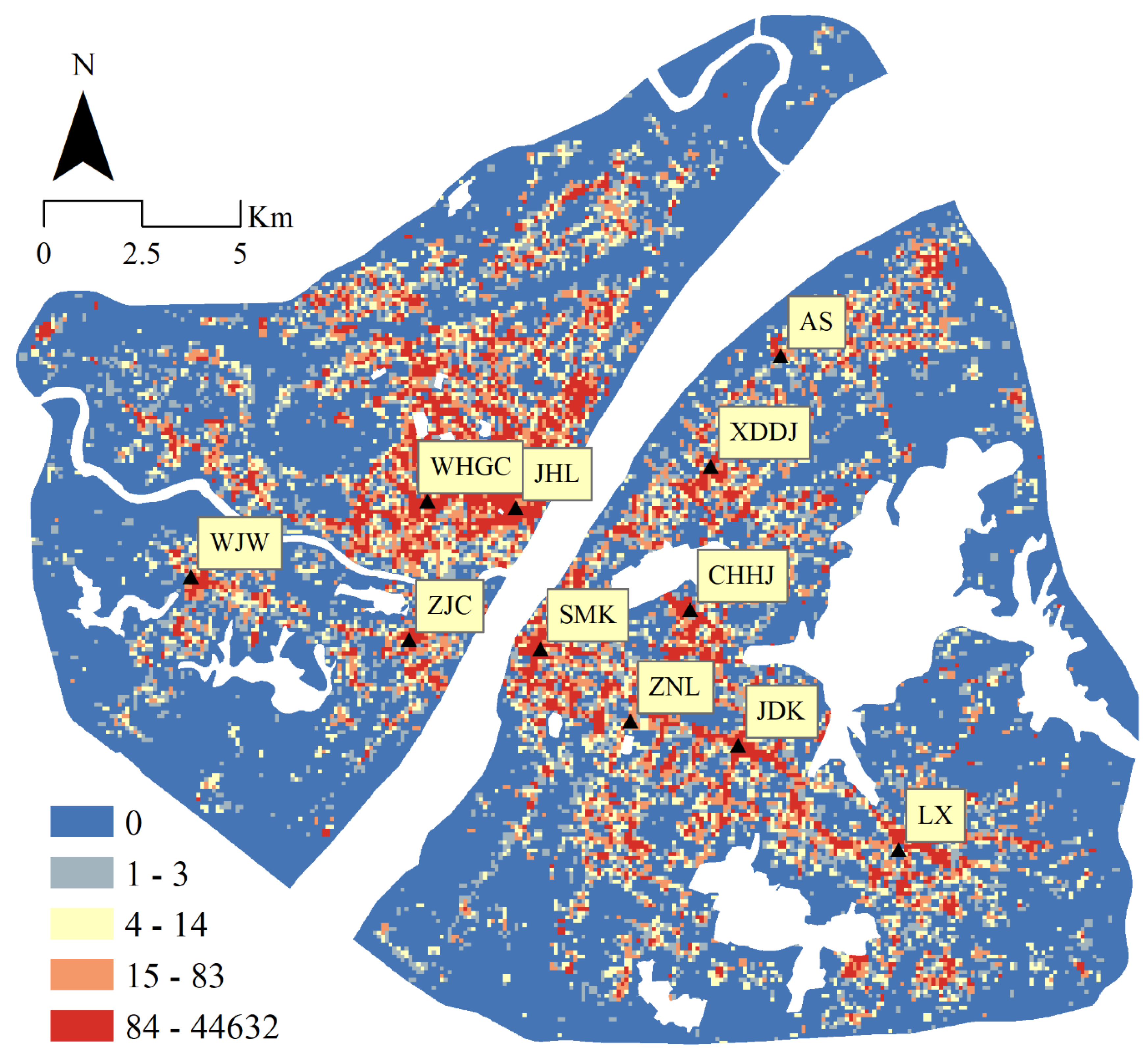
• Urban vitality demonstrated a high level of spatial agglomeration. Most regions with high vitality coincided in position with streets;
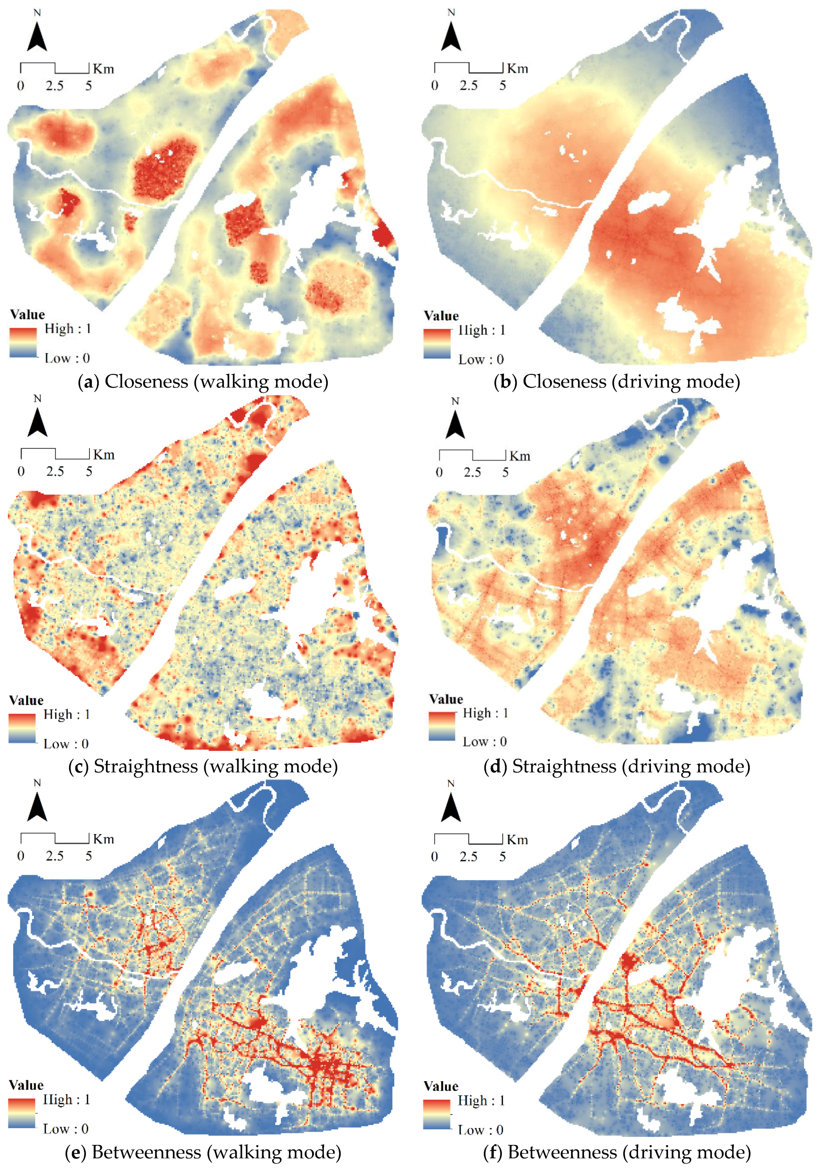
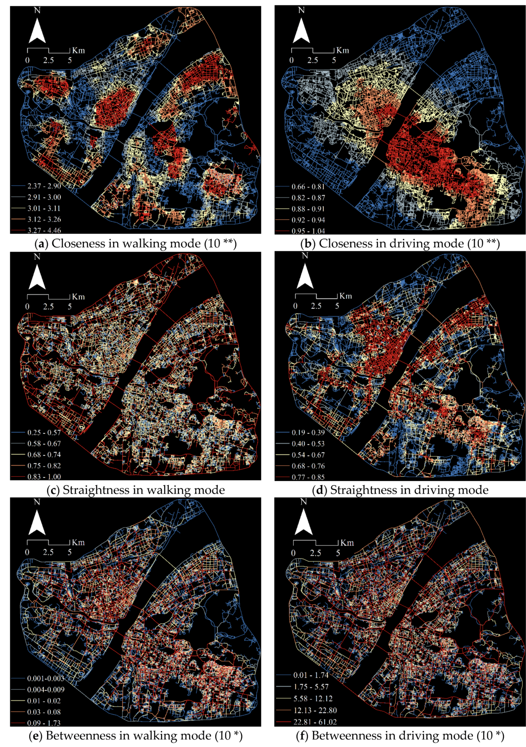
• Different street centralities had different distribution characteristics in space. Regions with high closeness in walking mode were gathered in several isolated clusters, while regions with high closeness in driving mode presented a monocentric pattern with the downtown as the center. Regions with high straightness in walking mode were dispersed in space, while regions with high straightness in driving mode were clustered along main roads. Regions with high betweenness in walking and driving modes coincided in position with main roads;
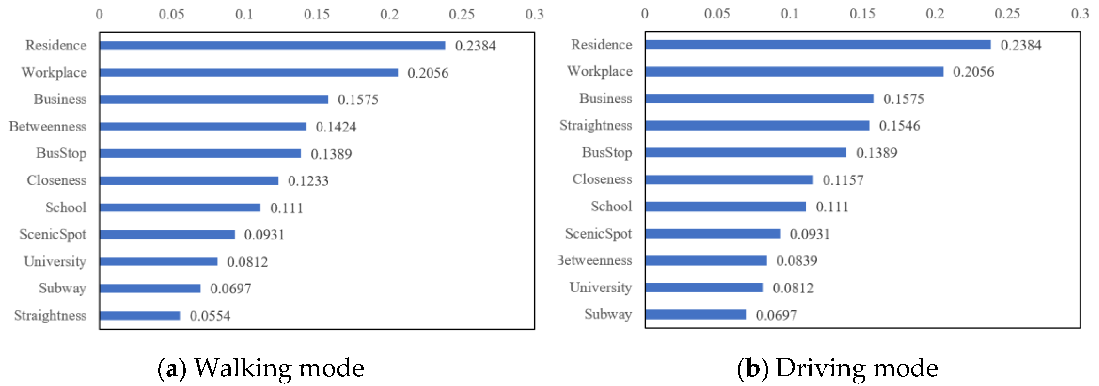
• Spatial association between urban vitality and street centrality in different travel modes was revealed. When considering street centrality in walking mode, betweenness had the most significant impact on urban vitality, followed by closeness and straightness. When considering street centrality in driving mode, however, straightness had the most significant impact, followed by closeness and betweenness.

The findings from this study have policy implications concerning the crucial role of street configuration in creating vibrant cities. First, an overall positive spatial association between street centrality and urban vitality demonstrated that spatial features of human activity, such as geographic location, are necessary for scientific urban planning. Authorities should make use of location advantages in a street network to guide the design of urban environments and allocate commercial establishments for city liveliness and economic prosperity. Second, urban designers and planners should be aware that the superiority of a street network configuration cannot be determined at a single scale, and on the contrary, they should consider multiple travel modes to accommodate different people’s preferences for trip modes.

This research still had some limitations. First, the calculation of street centrality was subject to the edge effect, i.e., the distortion that lowers centrality values near the edge of a district. Second, we used a fine and frequently used square mesh (with a cell size of 100 m × 100 m) to combine different datasets. There may have been a common modifiable areal unit problem: analytical results are sensitive to the definition of units in which data are collected. Third, social network review data have their own limitations in terms of representativeness and generalizability. Future studies should take these issues into consideration. Additionally, future research should compare the MCA model to the space syntax model, which is another popular structural interpretation of urban space.

References

1. Ye, Y.; Li, D.; Liu, X. How block density and typology affect urban vitality: An exploratory analysis in Shenzhen, China. Urban Geogr. 2018, 39, 631–652. [Google Scholar] [CrossRef]
2. Den Hartog, H. Shanghai New Towns: Searching for Community and Identity in a Sprawling Metropolis; 010 Publishers: Rotterdam, The Netherlands, 2010. [Google Scholar]
3. Chen, T.; Hui, E.C.M.; Wu, J.; Lang, W.; Li, X. Identifying urban spatial structure and urban vibrancy in highly dense cities using georeferenced social media data. Habitat Int. 2019, 89, 102005. [Google Scholar] [CrossRef]
4. Findlay, A.; Sparks, L. LR Policies Adopted to Support a Healthy Retail Sector; Scottish Government Social Research: Edinburgh, UK, 2009.
5. Jacobs, J. The Death and Life of Great American Cities; Random House: New York, NY, USA, 1961. [Google Scholar]
6. Montgomery, J. Making a city: Urbanity, vitality and urban design. J. Urban Des. 1998, 3, 93–116. [Google Scholar] [CrossRef]
7. Landry, C. Urban vitality: A new source of urban competitiveness. Archis 2000, 12, 8–13. [Google Scholar]
8. Li, M.; Shen, Z.; Hao, X. Revealing the relationship between spatio-temporal distribution of population and urban function with social media data. GeoJournal 2016, 81, 919–935. [Google Scholar] [CrossRef]
9. Jin, X.; Long, Y.; Sun, W.; Lu, Y.; Yang, X.; Tang, J. Evaluating cities’ vitality and identifying ghost cities in China with emerging geographical data. Cities 2017, 63, 98–109. [Google Scholar] [CrossRef]
10. Wang, F.; Guldmann, J.M. Simulating urban population density with a gravity-based model. Socio-Econ. Plan. Sci. 1996, 30, 245–256. [Google Scholar] [CrossRef]
11. Braun, L.M.; Malizia, E. Downtown vibrancy influences public health and safety outcomes in urban counties. J. Transp. Health 2015, 2, 540–548. [Google Scholar] [CrossRef]
12. Mellander, C.; Lobo, J.; Stolarick, K.; Matheson, Z. Night-Time Light Data: A Good Proxy Measure for Economic Activity? PLoS ONE 2015, 10, e0139779. [Google Scholar] [CrossRef]
13. Harvey, L. Defining and measuring employability. Qual. High. Educ. 2001, 7, 97–109. [Google Scholar] [CrossRef]
14. Nicodemus, A.G. Fuzzy vibrancy: Creative placemaking as ascendant US cultural policy. Cult. Trends 2013, 22, 213–222. [Google Scholar] [CrossRef]
15. Wang, T.; Wang, Y.; Zhao, X.; Fu, X. Spatial distribution pattern of the customer count and satisfaction of commercial facilities based on social network review data in Beijing, China. Comput. Environ. Urban Syst. 2018, 71, 88–97. [Google Scholar] [CrossRef]
16. Zeng, C.; Song, Y.; He, Q.; Shen, F. Spatially explicit assessment on urban vitality: Case studies in Chicago and Wuhan. Sustain. Cities Soc. 2018, 40, 296–306. [Google Scholar] [CrossRef]
17. Zukin, S. Naked City: The Death and Life of Authentic Urban Places; Oxford University Press: New York, NY, USA, 2010. [Google Scholar]
18. Roig-Tierno, N.; Baviera-Puig, A.; Buitrago-Vera, J.; Mas-Verdu, F. The retail site location decision process using GIS and the analytical hierarchy process. Appl. Geogr. 2013, 40, 191–198. [Google Scholar] [CrossRef]
19. Dawson, J.A. Retail Geography; Halsted Press: New York, NY, USA, 2013. [Google Scholar]
20. Philipsen, K. How Food Became the Ferment of Urbanity. Community Architecture Website 2015. Available online: http://archplanbaltimore.blogspot.sg/2015/10/how-food-became-ferment-of-urbanity.html (accessed on 25 May 2019).
21. Huang, Q.; Wong, D.W.S. Activity patterns, socioeconomic status and urban spatial structure: What can social media data tell us? Int. J. Geogr. Inf. Sci. 2016, 30, 1873–1898. [Google Scholar] [CrossRef]
22. Hu, Y.; Gao, S.; Janowicz, K.; Yu, B.; Li, W.; Prasad, S. Extracting and understanding urban areas of interest using geotagged photos. Comput. Environ. Urban Syst. 2015, 54, 240–254. [Google Scholar] [CrossRef]
23. Sun, Y.; Fan, H.; Li, M.; Zipf, A. Identifying the city center using human travel flows generated from location-based social networking data. Environ. Plan. B Plan. Des. 2016, 43, 480–498. [Google Scholar] [CrossRef]
24. Yue, Y.; Zhuang, Y.; Yeh, A.G.O.; Xie, J.-Y.; Ma, C.-L.; Li, Q.-Q. Measurements of POI-based mixed use and their relationships with neighbourhood vibrancy. Int. J. Geogr. Inf. Sci. 2017, 31, 658–675. [Google Scholar] [CrossRef]
25. Lefebvre, H. Writings on Cities; Blackwell Publishing: Oxford, UK, 1968. [Google Scholar]
26. Oliveira, V. Morpho: A methodology for assessing urban form. Urban Morphol. 2013, 17, 21–33. [Google Scholar]
27. Yue, H.; Zhu, X.; Ye, X.; Hu, T.; Kudva, S. Modelling the effects of street permeability on burglary in Wuhan, China. Appl. Geogr. 2018, 98, 177–183. [Google Scholar] [CrossRef]
28. Rui, Y.K.; Ban, Y.F. Exploring the relationship between street centrality and land use in Stockholm. Int. J. Geogr. Inf. Sci. 2014, 28, 1425–1438. [Google Scholar] [CrossRef]
29. Cui, C.; Wang, J.; Wu, Z.; Ni, J.; Qian, T. The Socio-Spatial Distribution of Leisure Venues: A Case Study of Karaoke Bars in Nanjing, China. ISPRS Int. J. Geo-Inf. 2016, 5, 150. [Google Scholar] [CrossRef]
30. Kang, C.-D. Measuring the effects of street network configurations on walking in Seoul, Korea. Cities 2017, 71, 30–40. [Google Scholar] [CrossRef]
31. Wang, F.; Antipova, A.; Porta, S. Street centrality and land use intensity in Baton Rouge, Louisiana. J. Transp. Geogr. 2011, 19, 285–293. [Google Scholar] [CrossRef] [Green Version]
32. He, S.; Yu, S.; Wei, P.; Fang, C. A spatial design network analysis of street networks and the locations of leisure entertainment activities: A case study of Wuhan, China. Sustain. Cities Soc. 2019, 44, 880–887. [Google Scholar] [CrossRef]
33. Lin, G.; Chen, X.; Liang, Y. The location of retail stores and street centrality in Guangzhou, China. Appl. Geogr. 2018, 100, 12–20. [Google Scholar] [CrossRef]
34. Wang, F.; Chen, C.; Xiu, C.; Zhang, P. Location analysis of retail stores in Changchun, China: A street centrality perspective. Cities 2014, 41, 54–63. [Google Scholar] [CrossRef]
35. Porta, S.; Crucitti, P.; Latora, V. The network analysis of urban streets: A primal approach. Environ. Plan. B Plan. Des. 2006, 33, 705–725. [Google Scholar] [CrossRef]
36. Borruso, G. Network density and the delimitation of urban areas. Trans. GIS 2003, 7, 177–191. [Google Scholar] [CrossRef]
37. Nes, A.V. Typology of shopping areas in Amsterdam. In Proceedings of the 5th International Symposium on Space Syntax, Delft, The Netherlands, 13–17 June 2005. [Google Scholar]
38. Hansen, W. How accessibility shapes land use. J. Am. Inst. Plan. 1959, 25, 73–76. [Google Scholar] [CrossRef]
39. Hillier, B. Space Is the Machine: A Configurational Theory of Architecture; Cambridge University Press: Cambridge, UK, 1996. [Google Scholar]
40. Porta, S.; Strano, E.; Iacoviello, V.; Messora, R.; Latora, V.; Cardillo, A.; Wang, F.; Scellato, S. Street centrality and densities of retail and services in Bologna, Italy. Environ. Plan. B Plan. Des. 2009, 36, 450–465. [Google Scholar] [CrossRef]
41. Anselin, L.; Bera, A. Spatial dependence in linear regression models with an introduction to spatial econometrics. In Handbook of Applied Economic Statistics; Ullah, A., Giles, D.E., Eds.; Marcel Dekker: New York, NY, USA, 1998; pp. 237–289. [Google Scholar]
42. National Bureau of Statistics of China. Wuhan Statistical Yearbook-2016; China Statistics Press: Beijing, China, 2016. [Google Scholar]
43. Jiang, B.; Claramunt, C. Topological Analysis of Urban Street Networks. Environ. Plan. B Plan. Des. 2004, 31, 151–162. [Google Scholar] [CrossRef] [Green Version]
44. Sabidussi, G. The centrality index of a graph. Psychometrika 1966, 31, 581–603. [Google Scholar] [CrossRef] [PubMed]
45. Dalton, R.C. The secret is to follow your nose: Route Path Selection and Angularity. Environ. Behav. 2003, 35, 107–131. [Google Scholar] [CrossRef]
46. Freeman, L.C. A set of measures of centrality based on betweenness. Sociometry 1977, 40, 35–41. [Google Scholar] [CrossRef]
47. Sevtsuk, A.; Mekonnen, M.; Kalvo, R. Urban Network Analysis: A Toolbox v1.01 for ArcGIS; Singapore University of Technology and Design: Singapore, 2013. [Google Scholar]
48. Ye, Y. Urban Form Index for Quantitative Urban Morphology and Urban Design Analyses. Ph.D. Thesis, University of Hong Kong, Hong Kong, China, September 2015. [Google Scholar]
49. Anselin, L. Local Indicators of Spatial Association—LISA. Geogr. Anal. 1995, 27, 93–115. [Google Scholar] [CrossRef]
50. Clifford, P.; Richardson, S. Testing the association between two spatial processes. Stat. Decis. 1985, 2, 155–160. [Google Scholar]
51. Wang, J.F.; Li, X.H.; Christakos, G.; Liao, Y.L.; Zhang, T.; Gu, X.; Zheng, X.Y. Geographical Detectors—Based Health Risk Assessment and its application in the neural tube defects study of the Heshun Region, China. Int. J. Geogr. Inf. Sci. 2010, 24, 107–127. [Google Scholar] [CrossRef]
52. Crane, R. Cars and drivers in the new suburbs: Linking access to travel in neotraditional planning. J. Am. Plan. Assoc. 1996, 62, 51–65. [Google Scholar] [CrossRef]
Figure 1. Location of the study area. (a) China; (b) Wuhan City; (c) Study area (urban area within the third ring road).
Sustainability 11 04356 g001
Figure 2. Spatial distribution of urban vitality. Abbreviations: WHGC = Wu Han Guang Chang, JHL = Jiang Han Lu, WJW = Wang Jia Wan, ZJC = Zhong Jia Cun, SMK = Si Men Kou, ZNL = Zhong Nan Lu, JDK = Jie Dao Kou, LX = Lu Xiang, AS = Ao Shan, XDDJ = Xu Dong Da Jie, CHHJ = Chu He Han Jie. These are major business districts in Wuhan.
Sustainability 11 04356 g002
Figure 3. Spatial distribution of street centrality. (a) Closeness (walking mode); (b) Closeness (driving mode); (c) Straightness (walking mode); (d) Straightness (driving mode); (e) Betweenness (walking mode); (f) Betweenness (driving mode).
Sustainability 11 04356 g003
Figure 4. Power of determinant for independent variables guiding the urban vitality effect with street centrality calculated in (a) walking mode, (b) driving mode. Abbreviations: Residence = gravity index of residence, Workplace = gravity index of workplace, Business = distance to the nearest business district, Bus Stop = distance to the nearest bus stop, School = distance to the nearest school, Scenic Spot = distance to the nearest scenic spot, University = distance to the nearest university, Subway = distance to the nearest subway station.
Sustainability 11 04356 g004