Scientific Decision Framework for Evaluation of Renewable Energy Sources under Q-Rung Orthopair Fuzzy Set with Partially Known Weight Information

Abstract

As an attractive generalization of the intuitionistic fuzzy set (IFS), q-rung orthopair fuzzy set (q-ROFS) provides the decision makers (DMs) with a wide window for preference elicitation. Previous studies on q-ROFS indicate that there is an urge for a decision framework which can make use of the available information in a proper manner for making rational decisions. Motivated by the superiority of q-ROFS, in this paper, a new decision framework is proposed, which provides scientific methods for multi-attribute group decision-making (MAGDM). Initially, a programming model is developed for calculating weights of attributes with the help of partially known information. Later, another programming model is developed for determining the weights of DMs with the help of partially known information. Preferences from different DMs are aggregated rationally by using the weights of DMs and extending generalized Maclaurin symmetric mean (GMSM) operator to q-ROFS, which can properly capture the interrelationship among attributes. Further, complex proportional assessment (COPRAS) method is extended to q-ROFS for prioritization of objects by using attributes’ weight vector and aggregated preference matrix. The applicability of the proposed framework is demonstrated by using a renewable energy source prioritization problem from an Indian perspective. Finally, the superiorities and weaknesses of the framework are discussed in comparison with state-of-the-art methods.

1. Introduction

Energy from fossil fuels such as coal, petroleum, and natural gas act as a dominant contributor to the economic development of the nation. Most countries in the world exploit these fuels to create massive globalization and expansion of the market. India makes a significant contribution to the global market with a total energy consumption of about 73.46% in 2014 (https://tradingeconomics.com/). In a recent survey by Indragandhi et al. [1], it was claimed that by 2040 fossil fuels will run out of inventory and countries have to switch to renewable energy sources for managing global demands. Pillai and Banerjee [2] made an analysis of renewable energy from India’s standpoint and found that India only consumes 4% of the world’s primary energy. Reddy and Painuly [3] and Indragandhi et al. [1] inferred from their analysis that India has a high scope for renewable energy sources and it can effectively manage energy crisis by proper planning and management. Recently, Mardani et al. [4] conducted a detailed analysis on the use of multi-attribute group decision-making (MAGDM) methods for solving energy management problems, and it can be inferred from the analysis that energy source evaluation and selection can be effectively solved by using MAGDM perspectives. Furthermore, there is uncertainty in the process of selection, which can be effectively managed by using fuzzy sets and its variants [5]. Baek and Lee et al. [6] proposed a new design strategy for optimal selection of renewable energy system (RES) in buildings. Gonzalez et al. [7] presented a conceptual model to understand the relationship among different factors that correspond to the sustainability and acceptance of RES projects. Cavallaro et al. [8,9] presented decision frameworks under intuitionistic fuzzy context to rationally select solar-hybrid power plants.

Motivated by these claims, in this paper, we propose a new decision framework for rational prioritization of renewable energy sources. The preference information used here is q-rung orthopair fuzzy set (q-ROFS) [10], which is a powerful generalization of the intuitionistic fuzzy set (IFS) [11] and Pythagorean fuzzy set [12]. q-ROFS provides a wider window to decision makers (DMs) for preference elicitation by relaxing the constraint (sum of the degree of membership and non-membership less than or equal to one). Inspired by the power of q-ROFS, many researchers used it for MAGDM applications. Yager and Alajlan [13] introduced q-ROFS for approximate reasoning. Later, Du [14] proposed different distance measures viz., Minkowski, Hamming, Euclidian, etc., under q-ROFS context and used the same for decision-making. Li et al. [15] provided a new variant for q-ROFS by combing the concept of picture fuzzy set [16] with q-ROFS and applied the same for decision-making. Liu et al. [17] extended the power Maclaurin symmetric mean operator to q-ROFS and used the same for MAGDM. Further, Wei et al. [18] and Liu et al. [19] extended the idea of Heronian mean and Bonferroni mean to q-ROFS context, respectively, and demonstrated its practicality by using MAGDM problems. Bai et al. [20] introduced partitioned Maclaurin symmetric mean operator for q-ROFS and applied it for MAGDM. Moreover, Wang et al. [21] presented q-ROFS based Muirhead mean operator and validated its usefulness from MAGDM problem.

From the brief review conducted above, following challenges can be inferred:

• A scientific decision framework which is comprised of aggregation operator for aggregating preferences, attributes’ weight calculation method, DMs’ weight calculation method, and ranking method is missing under the q-ROFS context;
• Aggregation operators that can properly capture the interrelationship among attributes are needed for effective aggregation of preferences under q-ROFS context;
• To the best of our knowledge, DMs’ weights are directly provided for aggregation in a q-ROFS context, which causes inaccuracies and imprecision in the decision-making process [22];
• Calculation of attributes’ weight values with the help of partially known information under q-ROFS context is an open challenge;
• Prioritization of objects by considering the nature of attributes is an interesting challenge under q-ROFS context.

To tackle these challenges, motivation is gained, and the contributions are presented below:

• A scientific decision framework is proposed under q-ROFS context, and it is used for effective prioritization of renewable energy sources;
• A new operator is proposed to aggregate preferences of DMs by extending generalized Maclaurin symmetric mean (GMSM) operator to q-ROFS. This operator not only captures the interrelationship among attributes but also utilizes a systematic procedure for calculating weights of the DMs;
• Koksalmis and Kabak [22] strongly emphasized the need for a systematic method for calculating DMs’ weight values. Inspired by the claim, in this paper, we propose a programming model under q-ROFS context for effectively determining DMs’ weights with the help of available partial information;
• Attributes’ weight values are also calculated sensibly by proposing a new programming model under q-ROFS context, which could use the partially known information effectively;
• Mousavi-Nasab et al. [23] conducted a comprehensive analysis of the complex proportional assessment (COPRAS) method with other methods and showcased its simplicity and advantage of handling prioritization from different angles. This inspired our focus on extending COPRAS for q-ROFS;
• Finally, the strengths and weaknesses of the proposed scientific decision framework are analyzed by comparison with other methods. Refer to Section 5 for details on references.

The rest of the paper is constructed as follows. Section 2 provides a preliminary review on some of the basic concepts of IFS and q-ROFS. In Section 3, the proposed decision framework is discussed in detail where the methods for calculating DMs’ and attributes’ weights are proposed along with methods for aggregation of preferences and prioritization of alternatives. Section 4 provides the numerical example of renewable energy source selection from the Indian perspective. Comparative analysis of the proposed framework with other methods is provided in Section 5, and Section 6 presents the concluding remarks and future directions.

2. Preliminaries

This section presents some basics of IFS and q-ROFS.

Definition 1

[9]. Let $U$ be a fixed set such that $T\subset U$ is also fixed. Now IFS $\tilde{T}$ is given by

$$\tilde{T}=\left(u,{\mu }_{\tilde{T}}\left(u\right),{\upsilon }_{\tilde{T}}\left(u\right)|uϵU\right),$$

(1)

where ${\mu }_{\tilde{T}}\left(u\right)$ is the degree of membership, ${\upsilon }_{\tilde{T}}\left(u\right)$ is the degree of non-membership. ${\mu }_{\tilde{T}}\left(u\right)\in \left[0,1\right]$, ${\upsilon }_{\tilde{T}}\left(u\right)\in \left[0,1\right]$, and ${\mu }_{\tilde{T}}\left(u\right)+{\upsilon }_{\tilde{T}}\left(u\right)\le 1$.

Definition 2

[8]. Let $U$ be a fixed set with $u$ being an element of $U$. $Q$ on $U$ is a q-ROFS given by

$$Q=\left(u,{\mu }_Q\left(u\right),{\upsilon }_Q\left(u\right)|uϵU\right),$$

(2)

where ${\mu }_Q\left(u\right)$ is the degree of membership, ${\upsilon }_{\tilde{T}}\left(u\right)$ is the degree of non-membership. ${\mu }_Q\left(u\right)\in \left[0,1\right]$, ${\upsilon }_Q\left(u\right)\in \left[0,1\right]$, ${\mu }_Q^q\left(u\right)+{\upsilon }_Q^q\left(u\right)\le 1$ with $q\ge 1$.

Here, $Q_i=\left({\mu }_i\left(u\right),{\upsilon }_i\left(u\right)\right)$ is a q-ROFN and the collection of such q-ROFNs forms the q-ROFS. Furthermore, ${\pi }_i^q=1-\left({\mu }_i^q+{\upsilon }_i^q\right)$ is called the degree of hesitation.

Definition 3

[8]. Let $Q_1$, $Q_2$ be two q-ROFNs, and the operational laws are given by

$$Q_1\oplus Q_2=\left({\left(1-\left(1-{\mu }_1^q\right)\left(1-{\mu }_2^q\right)\right)}^{1/q},{\upsilon }_1{\upsilon }_2\right),$$

(3)

$$Q_1^{\lambda }=\left({\mu }_1^{\lambda },{\left(1-{\left(1-{\upsilon }_1^q\right)}^{\lambda }\right)}^{1/q}\right),$$

(4)

$$Q_1\otimes Q_2=\left({\mu }_1{\mu }_2,{\left(1-\left(1-{\upsilon }_1^q\right)\left(1-{\upsilon }_2^q\right)\right)}^{1/q}\right),$$

(5)

$$\lambda Q_1=\left({\left(1-{\left(1-{\mu }_1^q\right)}^{\lambda }\right)}^{1/q},{\upsilon }_1^{\lambda }\right),\lambda >0,$$

(6)

$$S\left(Q_1\right)={\mu }^q-{\upsilon }^q,$$

(7)

$$A\left(Q_1\right)={\mu }^q+{\upsilon }^q,$$

(8)

$$Q_1^c=\left({\upsilon }_i,{\mu }_i\right),$$

(9)

where $S$ and $A$ are the score and accuracy measure of a q-ROFN.

3. Proposed Decision Framework

3.1. Programming Model for Attribute Weight Calculation

This section puts forward a new programming model for calculating the weights of the attributes. Common weight calculation methods are analytic hierarchy process (AHP) [24,25] and entropy measures [26,27] which determine weights when the information is completely unknown. Since the information about each attribute is partially known, a programming model is an effective way of using the information to calculate the weight values. Moreover, attributes’ weight calculation in the context of q-ROFS is an interesting area for exploration.

Motivated by these claims, in this section, we present the procedure for calculation weights of attributes using a newly proposed programming model.

Step 1: Construct a matrix with q-ROFNs of order $d\times n$ where $d$ represents the number of DMs and $n$ represents the number of attributes.

Step 2: Determine the positive ideal solution (PIS) and negative ideal solution (NIS) for each attribute using Equations (10) and (11).

$$Q_j^{+}=ma{x}_{j\in benefit}\left(A\left(Q_j\right)\right) or mi{n}_{j\in cost}\left(A\left(Q_j\right)\right)$$

(10)

$$Q_j^{-}=ma{x}_{j\in cost}\left(A\left(Q_j\right)\right) or mi{n}_{j\in benefit}\left(A\left(Q_j\right)\right)$$

(11)

where $A\left(Q_i\right)$ is the accuracy measure from Equation (8), $Q_j^{+}$ is the PIS value of the jth attribute and $Q_j^{-}$ is the NIS value of the jth attribute.

It must be noted that the PIS and NIS values are calculated for each attribute, and they are q-ROFNs.

Step 3: Use the PIS and NIS values from Step 2 to construct an objective function as given below:

Model 1:

$$Min Z={\displaystyle \sum }_{j=1}^n{\omega }_j{\displaystyle \sum }_{i=1}^m\left(d\left(Q_{ij},Q_j^{+}\right)-d\left(Q_{ij},Q_j^{-}\right)\right)$$

Subject to:

$$\begin{gathered} 0\le {\omega }_j\le 1 \\ {\displaystyle \sum }_j{\omega }_j=1 \end{gathered}$$

Here, the distance between two q-ROFNs is given by Equation (12).

$$d\left(Q_1,Q_2\right)=\sqrt{{\left({\left({\mu }_{ij}^q\right)}_{Q_1}-{\left({\mu }_{ij}^q\right)}_{Q_2}\right)}^2+{\left({\left({\upsilon }_{ij}^q\right)}_{Q_1}-{\left({\upsilon }_{ij}^q\right)}_{Q_2}\right)}^2+{\left({\left({\pi }_{ij}^q\right)}_{Q_1}-{\left({\pi }_{ij}^q\right)}_{Q_2}\right)}^2}$$

(12)

where $Q_1$ and $Q_2$ are two q-ROFNs.

3.2. Proposed Programming Model for DMs’ Weight Calculation

This section provides the proposed programming model for calculating DMs’ weight values. Most often, DMs’ weight values are directly provided as input, which causes inaccuracies in the decision-making process [28]. As argued by Koksalmis and Kabak [22], the calculation of DMs’ weight values is substantial for rational decision-making, and it prevents inaccuracies in the decision-making process.

Motivated by this claim, in this paper, efforts are made to calculate DMs’ weights in a systematic manner by making use of the partially available information. A programming model is proposed under q-ROFS context, and the procedure is given below:

Step 1: Obtain $d$ matrices of order $m\times n$ where $m$ is the number of alternatives, and $n$ is the number of attributes.

Step 2: Calculate the PIS and NIS values for each attribute by using Equations (13) and (14). The values are determined for all $d$ matrices.

$$Q_j^{PIS}=ma{x}_{j\in benefit}\left(A\left(Q_j\right)\right) or mi{n}_{j\in cost}\left(A\left(Q_j\right)\right)$$

(13)

$$Q_j^{NIS}=ma{x}_{j\in cost}\left(A\left(Q_j\right)\right) or mi{n}_{j\in benefit}\left(A\left(Q_j\right)\right)$$

(14)

where $Q_j^{PIS}$ is the PIS calculated for each attribute, $Q_j^{NIS}$ is the NIS calculated for each attribute.

It must be noted that Equations (13) and (14) are applied to all $d$ matrices.

Step 3: By using the result from Step 2, an objective function is formulated, which can be used for calculating the weights of the DMs.

Model 2:

$$Min Z={\displaystyle \sum }_{k=1}^d{w}_k\left(d\left(Q_{ij},Q_j^{PIS}\right)-d\left(Q_{ij},Q_j^{NIS}\right)\right)$$

Subject to:

$$\begin{gathered} 0\le w_k\le 1 \\ {\displaystyle \sum }_k{w}_k=1 \end{gathered}$$

Here, the distance is calculated by using Equation (15).

$$d\left(Q_1,Q_2\right)=\sqrt{{\displaystyle \sum }_{i=1}^m{\displaystyle \sum }_{j=1}^n\left({\left({\left({\mu }_{ij}^q\right)}_{Q_1}-{\left({\mu }_{ij}^q\right)}_{Q_2}\right)}^2+{\left({\left({\upsilon }_{ij}^q\right)}_{Q_1}-{\left({\upsilon }_{ij}^q\right)}_{Q_2}\right)}^2+{\left({\left({\pi }_{ij}^q\right)}_{Q_1}-{\left({\pi }_{ij}^q\right)}_{Q_2}\right)}^2\right)}$$

(15)

where $Q_1$ and $Q_2$ are any two q-ROFNs.

3.3. Proposed q-ROFGMSM Operator

This section provides a new extension to GMSM operator under q-ROFS context. The GMSM operator [29] is a generalization of Maclaurin symmetric mean (MSM) operator which can effectively capture the interrelationship between attributes. The GMSM operator can also readily derive other operators as special cases. q-ROFS [10] is an attractive generalization of IFS [11] which can provide a wider scope for DMs to offer their preferences.

Motivated by the superiority of GMSM operator and q-ROFS, in this paper, we propose q-rung orthopair fuzzy generalized Maclaurin symmetric mean (q-ROFGMSM) operator who utilizes the power of both q-ROFS and GMSM for aggregation of preferences.

Definition 4.

The q-ROFNs are aggregated using a q-ROFGMSM operator which produces a mapping$Q^n\to Q$given by

$$q-ROFGMS{M}^{\left(r,{\lambda }_1,\dots ,{\lambda }_r\right)}\left(Q_1, Q_2,\dots , Q_d\right)={\left({\left(1-{{\displaystyle \prod }}_{k=1}^d{\left(1-{{\displaystyle \prod }}_{l=1}^r{\left({\mu }_{ij}^q\right)}^{{\lambda }_l}\right)}^{w_k}\right)}^{\frac{1}{q}}\right)}^{\frac{1}{{{\displaystyle \sum }}_l{\lambda }_l}},$$

$${\left(1-{\left(1-{{\displaystyle \prod }}_{k=1}^d{\left(1-{{\displaystyle \prod }}_{l=1}^r{\left(1-{\upsilon }_{ij}^q\right)}^{{\lambda }_l}\right)}^{w_k}\right)}^{\frac{1}{{{\displaystyle \sum }}_l{\lambda }_l}}\right)}^{1/q},$$

(16)

where$⎡r=\frac{d}{2}⎤$is a parameter that determines the number of risk appetite values,${\lambda }_1,{\lambda }_2,\dots ,{\lambda }_r$is risk appetite values which can take possible values from the set$\left\{1,2,\dots ,d\right\}$,$w_k$is the weight of the$k^{th}$DM calculated by using the procedure given in Section 3.2.

Property 1.

Idempotency.

If q-ROFNs$Q_1=Q_2=\dots =Q_d=Q$then,$q-ROFGMS{M}^{\left(r,{\lambda }_1,\dots ,{\lambda }_r\right)}\left(Q_1,Q_2,\dots ,Q_d\right)=Q$.

Proof. 

From Equation (16), we get

$$q-ROFGMS{M}^{\left(r,{\lambda }_1,\dots ,{\lambda }_r\right)}\left(Q_1,Q_2,\dots ,Q_d\right)={\left({\left(1-{{\displaystyle \prod }}_{k=1}^d{\left(1-{{\displaystyle \prod }}_{l=1}^r{\left({\mu }_{ij}^q\right)}^{{\lambda }_l}\right)}^{w_k}\right)}^{\frac{1}{q}}\right)}^{\frac{1}{{{\displaystyle \sum }}_l{\lambda }_l}},$$

$${\left(1-{\left(1-{\displaystyle \prod }_{k=1}^d{\left(1-{\displaystyle \prod }_{l=1}^r{\left(1-{\upsilon }_{ij}^q\right)}^{{\lambda }_l}\right)}^{w_k}\right)}^{\frac{1}{{{\displaystyle \sum }}_l{\lambda }_l}}\right)}^{1/q},$$

By expanding the risk appetite, we get

$$q-ROFGMS{M}^{\left(r,{\lambda }_1,\dots ,{\lambda }_r\right)}\left(Q_1,Q_2,\dots ,Q_d\right)={\left({\left(1-{{\displaystyle \prod }}_{k=1}^d{\left(1-{{\displaystyle \prod }}_{l=1}^r{\left({\mu }_{ij}^q\right)}^{{\lambda }_1+{\lambda }_2+\dots +{\lambda }_r}\right)}^{w_k}\right)}^{\frac{1}{q}}\right)}^{\frac{1}{{{\displaystyle \sum }}_l{\lambda }_l}},$$

$${\left(1-{\left(1-{{\displaystyle \prod }}_{k=1}^d{\left(1-{{\displaystyle \prod }}_{l=1}^r{\left(1-{\upsilon }_{ij}^q\right)}^{{\lambda }_1+{\lambda }_2+\dots +{\lambda }_r}\right)}^{w_k}\right)}^{\frac{1}{{{\displaystyle \sum }}_l{\lambda }_l}}\right)}^{1/q}.$$

Similarly DMs’ weights are expanded and since ${\displaystyle \sum }_k{w}_k=1$, we get

$$q-ROFGMS{M}^{\left(r,{\lambda }_1,\dots ,{\lambda }_r\right)}\left(Q_1,Q_2,\dots ,Q_d\right)={\left({\left(1-{{\displaystyle \prod }}_{k=1}^d\left(1-{{\displaystyle \prod }}_{l=1}^r{\left({\mu }_{ij}^q\right)}^{{\lambda }_1+{\lambda }_2+\dots +{\lambda }_r}\right)\right)}^{\frac{1}{q}}\right)}^{\frac{1}{{{\displaystyle \sum }}_l{\lambda }_l}},$$

$${\left(1-{\left(1-{{\displaystyle \prod }}_{k=1}^d\left(1-{{\displaystyle \prod }}_{l=1}^r{\left(1-{\upsilon }_{ij}^q\right)}^{{\lambda }_1+{\lambda }_2+\dots +{\lambda }_r}\right)\right)}^{\frac{1}{{{\displaystyle \sum }}_l{\lambda }_l}}\right)}^{\frac{1}{q}}=Q.$$

 □

Property 2.

Commutativity.

If q-ROFNs$Q_i^{*}$are any permutation of$Q_i \forall i=1,2,\dots ,d$then,$q-ROFGMS{M}^{\left(r,{\lambda }_1,\dots ,{\lambda }_r\right)}\left(Q_1,Q_2,\dots ,Q_d\right)=q-ROFGMS{M}^{\left(r,{\lambda }_1,\dots ,{\lambda }_r\right)}\left(Q_1^{*},Q_2^{*},\dots ,Q_d^{*}\right)$.

Proof. 

Since $Q_i^{*}$ are any permutation of $Q_i \forall i=1,2,\dots ,d$, we get

$$q-ROFGMS{M}^{\left(r,{\lambda }_1,\dots ,{\lambda }_r\right)}\left(Q_1^{*},Q_2^{*},\dots ,Q_d^{*}\right)={\left({\left(1-{{\displaystyle \prod }}_{k=1}^d{\left(1-{{\displaystyle \prod }}_{l=1}^r{\left({\mu }_{ij}^{*q}\right)}^{{\lambda }_1+{\lambda }_2+\dots +{\lambda }_r}\right)}^{w_k}\right)}^{\frac{1}{q}}\right)}^{\frac{1}{{{\displaystyle \sum }}_l{\lambda }_l}},$$

$${\left(1-{\left(1-{{\displaystyle \prod }}_{k=1}^d{\left(1-{{\displaystyle \prod }}_{l=1}^r{\left(1-{\upsilon }_{ij}^{*q}\right)}^{{\lambda }_1+{\lambda }_2+\dots +{\lambda }_r}\right)}^{w_k}\right)}^{\frac{1}{{{\displaystyle \sum }}_l{\lambda }_l}}\right)}^{\frac{1}{q}},$$

$$={\left({\left(1-{{\displaystyle \prod }}_{k=1}^d{\left(1-{{\displaystyle \prod }}_{l=1}^r{\left({\mu }_{ij}^q\right)}^{{\lambda }_1+{\lambda }_2+\dots +{\lambda }_r}\right)}^{w_k}\right)}^{\frac{1}{q}}\right)}^{\frac{1}{{{\displaystyle \sum }}_l{\lambda }_l}},$$

$${\left(1-{\left(1-{{\displaystyle \prod }}_{k=1}^d{\left(1-{{\displaystyle \prod }}_{l=1}^r{\left(1-{\upsilon }_{ij}^q\right)}^{{\lambda }_1+{\lambda }_2+\dots +{\lambda }_r}\right)}^{w_k}\right)}^{\frac{1}{{{\displaystyle \sum }}_l{\lambda }_l}}\right)}^{\frac{1}{q}}=q-ROFGMS{M}^{\left(r,{\lambda }_1,\dots ,{\lambda }_r\right)}\left(Q_1,Q_2,\dots ,Q_d\right),$$

 □

Property 3.

Monotonicity.

If$Q_i^{\prime }$is another collection of q-ROFNs such that$Q_i^{\prime }\ge Q_i\forall i=1,2,\dots ,d$then,$q-ROFGMS{M}^{\left(r,{\lambda }_1,\dots ,{\lambda }_r\right)}\left(Q_1,Q_2,\dots ,Q_d\right)\le q-ROFGMS{M}^{\left(r,{\lambda }_1,\dots ,{\lambda }_r\right)}\left(Q_1^{\prime },Q_2^{\prime },\dots ,Q_d^{\prime }\right)$.

Proof. 

Consider ${\mu }_i^{\prime }={\left({\left(1-{{\displaystyle \prod }}_{k=1}^d{\left(1-{{\displaystyle \prod }}_{l=1}^r{\left({\mu }_{ij}^{*q}\right)}^{{\lambda }_1+{\lambda }_2+\dots +{\lambda }_r}\right)}^{w_k}\right)}^{\frac{1}{q}}\right)}^{\frac{1}{{{\displaystyle \sum }}_l{\lambda }_l}}$ and ${\upsilon }_i^{\prime }={\left(1-{\left(1-{{\displaystyle \prod }}_{k=1}^d{\left(1-{{\displaystyle \prod }}_{l=1}^r{\left(1-{\upsilon }_{ij}^{*q}\right)}^{{\lambda }_1+{\lambda }_2+\dots +{\lambda }_r}\right)}^{w_k}\right)}^{\frac{1}{{{\displaystyle \sum }}_l{\lambda }_l}}\right)}^{\frac{1}{q}}$.

The q-ROFNs $Q_i$ is also defined similarly. Let $q-ROFGMS{M}^{\left(r,{\lambda }_1,\dots ,{\lambda }_r\right)}\left(Q_1,Q_2,\dots ,Q_d\right)=Q$ and $q-ROFGMS{M}^{\left(r,{\lambda }_1,\dots ,{\lambda }_r\right)}\left(Q_1^{\prime },Q_2^{\prime },\dots ,Q_d^{\prime }\right)=Q^{\prime }$ and $Q_i^{\prime }\ge Q_i\forall i=1,2,\dots ,d$. By using score and accuracy measures from Equations. (7) and (8), if $S\left(Q\right)\ge S\left(Q^{\prime }\right)$ then, $Q\ge Q^{\prime }$. When $S\left(Q\right)=S\left(Q^{\prime }\right)$ then, calculate accuracy. If $A\left(Q\right)\ge A\left(Q^{\prime }\right)$ then, $Q\le Q^{\prime }$. Thus, $q-ROFGMS{M}^{\left(r,{\lambda }_1,\dots ,{\lambda }_r\right)}\left(Q_1,Q_2,\dots ,Q_d\right)\le q-ROFGMS{M}^{\left(r,{\lambda }_1,\dots ,{\lambda }_r\right)}\left(Q_1^{\prime },Q_2^{\prime },\dots ,Q_d^{\prime }\right)$. □

Property 4.

Boundedness.

If$Q^{-}=mi{n}_i\left(Q_i\right)$and$Q^{+}=ma{x}_i\left(Q_i\right)$ then, $Q^{-}\le q-ROFGMS{M}^{\left(r,{\lambda }_1,\dots ,{\lambda }_r\right)}\left(Q_1, Q_2,\dots ,Q_d\right)\le Q^{+}$.

Proof. 

By monotonicity and idempotency, we get

$$q-ROFGMS{M}^{\left(r,{\lambda }_1,\dots ,{\lambda }_r\right)}\left(Q_1,Q_2,\dots ,Q_d\right)\le q-ROFGMS{M}^{\left(r,{\lambda }_1,\dots ,{\lambda }_r\right)}\left(Q^{+},Q^{+},\dots ,Q^{+}\right),$$

$$q-ROFGMS{M}^{\left(r,{\lambda }_1,\dots ,{\lambda }_r\right)}\left(Q_1,Q_2,\dots ,Q_d\right)\ge q-ROFGMS{M}^{\left(r,{\lambda }_1,\dots ,{\lambda }_r\right)}\left(Q^{-},Q^{-},\dots ,Q^{-}\right).$$

By integrating, we get

$$Q^{-}\le q-ROFGMS{M}^{\left(r,{\lambda }_1,\dots ,{\lambda }_r\right)}\left(Q_1,Q_2,\dots ,Q_d\right)\le Q^{+}.$$

 □

Theorem 1.

Aggregation of q-ROFNs using q-ROFGMSM operator produces a q-ROFN.

Proof. 

To prove the theorem, we need to show that the result of q-ROFGMSM operator follows Definition 2. From Property 4, it is clear that the proposed operator produces a result, which is bounded. That is, $Q^{-}\le q-ROFGMS{M}^{\left(r,{\lambda }_1,\dots ,{\lambda }_r\right)}\left(Q_1, Q_2,\dots ,Q_d\right)\le Q^{+}$. By generalizing the idea, we get $0\le {\left({\left(1-{{\displaystyle \prod }}_{k=1}^d{\left(1-{{\displaystyle \prod }}_{l=1}^r{\left({\mu }_{ij}^q\right)}^{{\lambda }_l}\right)}^{w_k}\right)}^{\frac{1}{q}}\right)}^{\frac{1}{{{\displaystyle \sum }}_l{\lambda }_l}}\le 1$ and $0\le {\left(1-{\left(1-{{\displaystyle \prod }}_{k=1}^d{\left(1-{{\displaystyle \prod }}_{l=1}^r{\left(1-{\upsilon }_{ij}^q\right)}^{{\lambda }_1+{\lambda }_2+\dots +{\lambda }_r}\right)}^{w_k}\right)}^{\frac{1}{{{\displaystyle \sum }}_l{\lambda }_l}}\right)}^{\frac{1}{q}}\le 1$.

By integrating, we get

$$0\le {\left({\left(1-{{\displaystyle \prod }}_{k=1}^d{\left(1-{{\displaystyle \prod }}_{l=1}^r{\left({\mu }_{ij}^q\right)}^{{\lambda }_l}\right)}^{w_k}\right)}^{\frac{1}{q}}\right)}^{\frac{1}{{{\displaystyle \sum }}_l{\lambda }_l}}+{\left(1-{\left(1-{{\displaystyle \prod }}_{k=1}^d{\left(1-{{\displaystyle \prod }}_{l=1}^r{\left(1-{\upsilon }_{ij}^q\right)}^{{\lambda }_1+{\lambda }_2+\dots +{\lambda }_r}\right)}^{w_k}\right)}^{\frac{1}{{{\displaystyle \sum }}_l{\lambda }_l}}\right)}^{\frac{1}{q}}\le {\displaystyle \sum }_k{w}_k=1.$$

Thus, the aggregation of q-ROFNs using q-ROFGMSM operator produces a q-ROFN. □

3.4. q-ROFS Based COPRAS Method

This section puts forward a new extension to COPRAS ranking method under q-ROFS context. COPRAS method was initially developed by Zavadskas et al. [30]. Later, Zavadskas et al.’s method [31] was applied for the evaluation of dwellers for walls. Further, a comprehensive review was made on different ranking methods, and it was inferred that the COPRAS ranking method was simple, effective, and rational for various MAGDM problems [32]. Inspired by these desirable properties of COPRAS, many researchers extended the method for different MAGDM problems. Mondal et al. [33], Vahdani et al. [34], and Gorabe et al. [35] extended the COPRAS method for the evaluation and selection of industrial robots. Zavadskas et al. [36,37] introduced gray COPRAS method and used the same for the evaluation of project managers and contractors. Razavi Hajiagha et al. [38] and Wang et al. [39] proposed interval-valued intuitionistic fuzzy COPRAS method for investor selection problem. Valipour et al. [40] presented a hybrid method by integrating SWARA (step-wise weight assessment ratio analysis) with the COPRAS method and used the same for risk evaluation in the excavation project. Recently, Mardani et al. [41] conducted an interesting survey on various utility-based MCDM methods, including COPRAS, and presented several application areas under the MCDM context. Following this, Stefano et al. [42] conducted a deep review of the COPRAS method and demonstrated its variants and use in many MCDM problems. Bielinskas et al. [43] put forward a new strategic decision framework for the selection of a suitable scenario for urban brownfield using COPRAS method. Yazdani et al. [44] proposed a hybrid model for the evaluation of green suppliers by using quality functional deployment (QFD) and the COPRAS method. Bausys et al. [45] presented an interesting extension of COPRAS to neutrosophic fuzzy set and demonstrated its use in MAGDM. Roy et al. [46] proposed a decision-making method for hotel selection by extending the COPRAS method under weighted rough context. Ayrum et al. [47] gave a new extension to the COPRAS method under the stochastic model and applied the same to decision-making problems. Moreover, Chatterjee et al. [48,49] and Mousavi-Nasab et al. [23] extended the COPRAS method for material selection. Zheng et al. [50] proposed a hesitant fuzzy linguistic COPRAS method and applied the same for medical application. Chatterjee and Kar [5,51] presented a hybrid model by extending the COPRAS method fuzzy and Z-number context and used the same for the evaluation of the telecommunication industry and renewable energy sources.

From the brief analysis made above, it is clear that the COPRAS method is a simple, effective, and rational method for decision-making. Furthermore, it can be inferred that the COPRAS method ranks objects from different angles and considers the direct and proportional relationship between objects and attributes. Motivated by the superiority of the COPRAS method, in this section, we extend the method for q-ROFS context. The procedure for the proposed q-ROFS based COPRAS method is given below:

Step 1: Get a decision matrix of order $m\times n$ where $m$ denotes the number of alternatives and $n$ denotes the number of attributes with PLTS information.

Step 2: Obtain the weight vector of the attributes (refer Section 3.1) for calculating the ranks of the alternatives.

Step 3: Determine the COPRAS parameters $P_i$ and $R_i$ by using Equations (17) and (18).

$$P_i={\omega }_j{Q}_{ij}{\oplus }_{j=1}^{\#benefit}{\omega }_{j+1}{Q}_{i\left(j+1\right)}\forall j=1,2,\dots ,n$$

(17)

$$R_i={\omega }_j{Q}_{ij}{\oplus }_{j=1}^{\#cost}{\omega }_{j+1}{Q}_{i\left(j+1\right)}\forall j=1,2,\dots ,n$$

(18)

where ${\omega }_j$ is the weight of the $j^{th}$ attribute, ${\omega }_{j+1}$ is the weight of the next attribute, $Q_{ij}$ is the q-ROFN of the $i^{th}$ alternative, and $j^{th}$ attribute and $Q_{i\left(j+1\right)}$ is the q-ROFN of the $i^{th}$ alternative and next attribute.

It must be noted that the process occurs for every attribute over a specific alternative.

Step 4: Calculate the $T{R}_i$ by using Equation (19) to determine the prioritization order of alternatives.

$$T{R}_i=\phi A\left(P_i\right)+\left(1-\phi \right)\frac{{{\displaystyle \sum }}_{i=1}^{m}A\left(R_i\right)}{A\left(R_i\right)\left(\frac{1}{{{\displaystyle \sum }}_{i=1}^{m}A\left(R_i\right)}\right)}$$

(19)

where $\phi$ is the strategy value of the DM in unit interval.

The physical interpretation of strategy value is that when $\phi <0.5$, the DM is pessimistic in nature and hence, high value is associated as weight to the cost type attributes. On the other hand, when $\phi >0.5$, the DM is optimistic in nature and hence, high value is associated as weight to the benefit type attributes. Finally, when $\phi =0.5$, the DM is neutral in nature and equal weight is associated with both benefit and cost type attributes. This realization can be easily inferred from Equations (17)–(19). It must be noted that $P_i$ is with respect to benefit type attributes and $R_i$ is with respect to cost type attributes. $T{R}_i$ values are determined for each alternative, and they are arranged in descending order to form the prioritization vector.

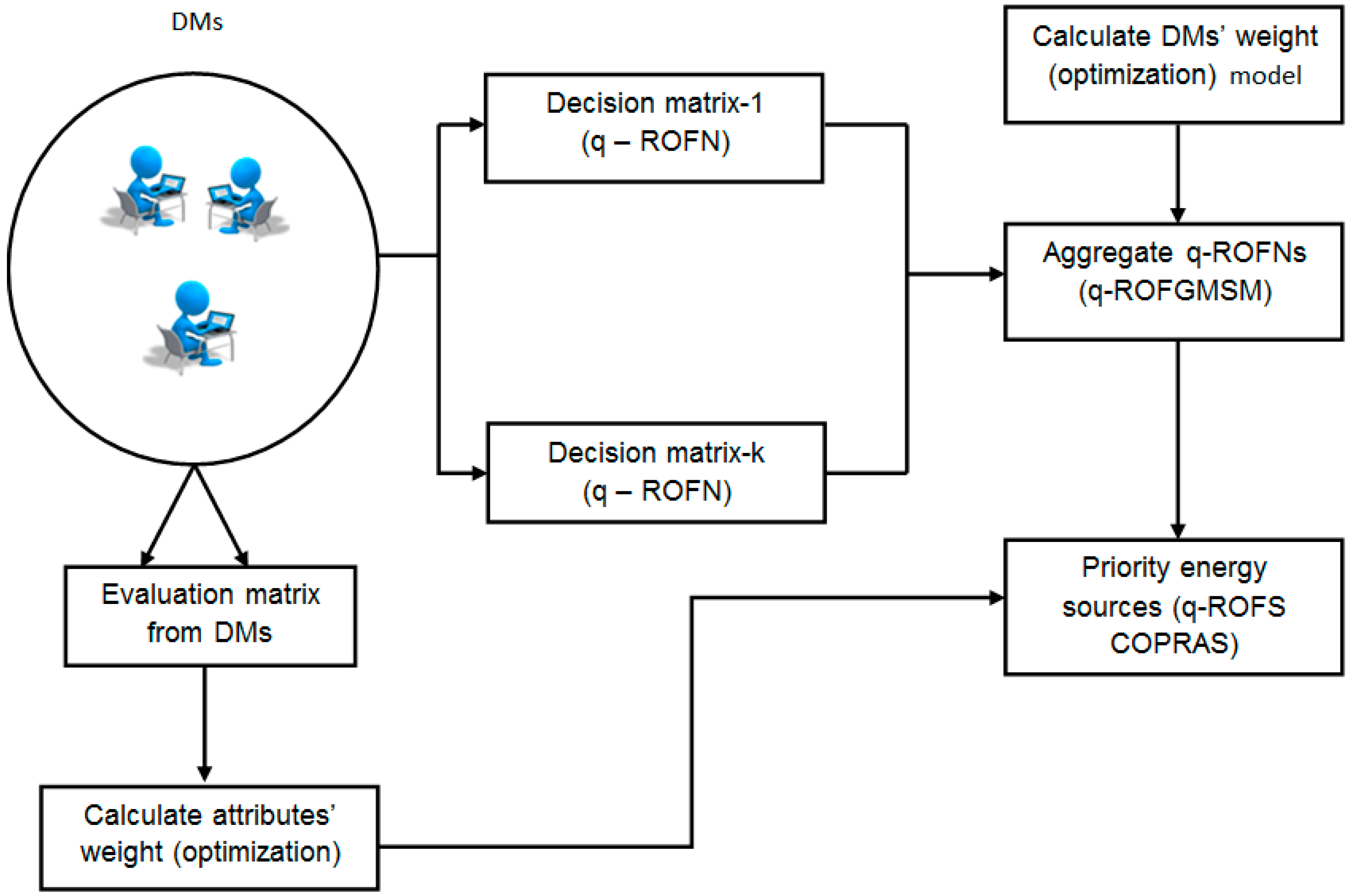
Figure 1 shows the working model of the proposed decision framework under q-ROFS context.

• Each DM provides a decision matrix of order $\mathit{m}\mathbf{\times }\mathit{n}$ with q-ROFNs as preferences. Here, $\mathit{m}$ represents the number of alternatives/objects and $\mathit{n}$ represents the number of attributes considered for evaluation of these alternatives/objects;
• These matrices are aggregated into a single decision matrix of order $\mathit{m}\mathbf{\times }\mathit{n}$ by using a q-ROFGMSM operator. This operator uses DMs’ weights as input, which are calculated in a systematic manner by using proposed programming model. The operator captures the interrelationship among attributes effectively;
• Later, DMs provide an evaluation matrix of order $\mathit{d}\mathbf{\times }\mathit{n}$, ($\mathit{d}$ represents the number of DMs and $\mathit{n}$ represents the number of attributes) for calculating the weights of the attributes using proposed programming model;
• The aggregated matrix of order $\mathit{m}\mathbf{\times }\mathit{n}$ and the weight vector of order $\mathit{1}\mathbf{\times }\mathit{n}$ are used as input to prioritize the energy sources by extending the popular COPRAS method under q-ROFS context. A vector of order $\mathit{1}\mathbf{\times }\mathit{m}$ is obtained as the prioritization order. The main advantage of the proposed ranking method is that it mitigates information loss effectively by properly retaining the q-rung orthopair fuzzy information throughout the study;
• Finally, the comparison is done to analyze the strengths and weaknesses of the proposed framework.

4. Illustrative Examples of Renewable Energy Source Selection

This section puts forward an illustrative example of renewable energy source selection under the Indian perspective. India owing to its diversified set of population and technological advancements, seek high demand for energy. Due to deep exploitation of traditional form of energy sources like coal, petroleum, and natural gas, there is a tremendous deal of energy crisis in the world. As discussed earlier, Indragandhi et al. [1] argued that by 2040, there would be an urge for renewable forms of energy to meet out the demands of the fast-growing country. They also claimed that the traditional resources would reach its limits by close 2050 due to wider exploitation and usage of such resources. Moreover, Chatterjee and Kar [5] presented the substantial need for a renewable energy source in India and identified potential attributes for evaluating the energy sources. We adapt the attributes from [5] for this study, and they are given by energy efficiency $z_1$, job creation $z_2$, the complexity of technology $z_3$, land usage $z_4$, CO₂ emission $z_5$, and total cost $z_6$. A brief description on each of these attributes is given below:

• Energy efficiency: This attribute defines the energy obtained from a renewable energy source, by considering the second law of thermodynamics. It is placed in benefit category as energy efficiency is expected to be high;
• Job creation: This attribute defines the job opportunities created by the renewable energy source supply, starting from installation to maintenance. From [5], it is clear that it is a substantial attribute to be considered and it is placed in benefit category as opportunities are expected to be high;
• Complexity of technology: This attribute defines the complexity involved in bringing a renewable energy based technology to practice. It includes geographic restrictions, lack of technology transfer, and structural complexity. Since the idea of renewable energy source has just started in India, evaluation from this perspective is important. It is placed in cost type as complexity is expected to be low;
• Land usage: This attribute defines the judicious usage of land by a renewable energy source. From [5], it is clear that different energy sources need different land space and hence, this attribute is placed in benefit type. Due to the population of India, judicious land usage is highly encouraged;
• CO₂ emission: The major factor for global warming is carbon-dioxide and hence, this attribute is used to measure the amount of carbon-dioxide emitted by different energy source. Obviously, it is placed in cost type;
• Total cost: This attribute defines the overall cost incurred by an energy source, starting from the installation, maintenance, to the final delivery to customers. Obviously, this attribute is also placed in cost type.

Further from the research of Luthra et al. [52], we chose suitable sources of energy under Indian context, and they are given by tidal $e{s}_1$, geothermal $e{s}_2$, solar $e{s}_3$, wind $e{s}_4$, and hydrogen $e{s}_5$. Three DMs are chosen for evaluation viz., $d_1$, $d_2$, and $d_3$ who have high experience in the field of sustainable energy science and energy resource selection and evaluation. These DMs rate the sources over each attribute and use q-ROFNs.

Example 1.

Renewable energy source selection.

The procedure for rational decision-making with the help of a proposed decision framework is given below:

Step 1: Begin.

Step 2: Construct three decision matrices with q-ROFNs, and their order is given by $5\times 6$ (refer to

Table 1. Decision makers’ (DMs) preference information under q-ROFS context.

Evaluation Attributes for Energy Sources
Energy Sources	${\mathit{z}}_1$	${\mathit{z}}_2$	${\mathit{z}}_3$	${\mathit{z}}_4$	${\mathit{z}}_5$	${\mathit{z}}_6$
$d_1$
$e{s}_1$	(0.69,0.43)	(0.26,0.70)	(0.61,0.83)	(0.11,0.82)	(0.55,0.36)	(0.58,0.75)
$e{s}_2$	(0.28,0.31)	(0.53,0.59)	(0.66,0.39)	(0.14,0.24)	(0.26,0.57)	(0.51,0.47)
$e{s}_3$	(0.76,0.72)	(0.73,0.43)	(0.84,0.12)	(0.13,0.50)	(0.60,0.16)	(0.29,0.34)
$e{s}_4$	(0.13,0.43)	(0.46,0.69)	(0.66,0.62)	(0.41,0.88)	(0.46,0.45)	(0.74,0.24)
$e{s}_5$	(0.66,0.81)	(0.39,0.15)	(0.16,0.44)	(0.25,0.60)	(0.79,0.29)	(0.74,0.49)
$d_2$
$e{s}_1$	(0.63,0.16)	(0.20,0.88)	(0.87,0.29)	(0.54,0.54)	(0.42,0.77)	(0.37,0.14)
$e{s}_2$	(0.23,0.13)	(0.63,0.36)	(0.64,0.27)	(0.71,0.28)	(0.37,0.75)	(0.50,0.44)
$e{s}_3$	(0.84,0.28)	(0.12,0.85)	(0.35,0.48)	(0.34,0.72)	(0.46,0.60)	(0.52,0.69)
$e{s}_4$	(0.57,0.14)	(0.65,0.77)	(0.79,0.20)	(0.27,0.86)	(0.31,0.17)	(0.26,0.23)
$e{s}_5$	(0.86,0.50)	(0.50,0.65)	(0.69,0.67)	(0.50,0.36)	(0.11,0.12)	(0.45,0.17)
$d_3$
$e{s}_1$	(0.17,0.77)	(0.72,0.29)	(0.32,0.28)	(0.17,0.19)	(0.29,0.75)	(0.80,0.68)
$e{s}_2$	(0.48,0.67)	(0.22,0.30)	(0.17,0.52)	(0.86,0.67)	(0.86,0.39)	(0.27,0.66)
$e{s}_3$	(0.58,0.50)	(0.72,0.48)	(0.77,0.29)	(0.52,0.66)	(0.48,0.34)	(0.32,0.53)
$e{s}_4$	(0.83,0.41)	(0.58,0.57)	(0.76,0.48)	(0.44,0.13)	(0.84,0.36)	(0.34,0.34)
$e{s}_5$	(0.56,0.37)	(0.84,0.35)	(0.62,0.53)	(0.37,0.11)	(0.37,0.57)	(0.45,0.44)

Note: The preferences given by each DM is a q-ROFN. It has the form $\left({\mu }_{ij},{\upsilon }_{ij}\right)$ where ${\mu }_{ij}$ is the degree of membership/preference and ${\upsilon }_{ij}$ is the degree of non-membership/non-preference. As an example, the physical interpretation of an instance (0.69,0.43) by the DM $d_1$ is that the energy source $e{s}_1$ has a preference value of 0.69 and a non-preference value of 0.43 with respect to the attribute $z_1$.

).

From Table 1, the PIS and NIS values (from Equations (13) and (14)) for each attribute are calculated over each DM, and it is shown in

Table 2. Ideal solutions for each attribute from each DM.

Ideal Solution	Evaluation Attributes for Energy Sources
	${\mathit{z}}_1$	${\mathit{z}}_2$	${\mathit{z}}_3$	${\mathit{z}}_4$	${\mathit{z}}_5$	${\mathit{z}}_6$
PIS	(0.76,0.72)	(0.73,0.43)	(0.61,0.83)	(0.41,0.88)	(0.60,0.16)	(0.29,0.34)
NIS	(0.13,0.43)	(0.39,0.15)	(0.16,0.44)	(0.14,0.24)	(0.79,0.29)	(0.58,0.75)
PIS	(0.86,0.50)	(0.65,0.77)	(0.69,0.67)	(0.27,0.86)	(0.11,0.12)	(0.26,0.23)
NIS	(0.23,0.13)	(0.12,0.85)	(0.35,0.48)	(0.50,0.36)	(0.42,0.77)	(0.52,0.69)
PIS	(0.83,0.41)	(0.72,0.48)	(0.76,0.48)	(0.86,0.67)	(0.48,0.34)	(0.34,0.34)
NIS	(0.56,0.37)	(0.22,0.30)	(0.32,0.28)	(0.17,0.19)	(0.86,0.39)	(0.80,0.68)

Note: The positive ideal solution (PIS) and negative ideal solution (NIS) values are determined for each attribute for every decision matrix provided by the DMs. By applying Equations (13) and (14), the results are straightforward. q-ROFN that is associated with the corresponding accuracy value is considered as PIS and NIS for each attribute. The physical interpretation of PIS for an attribute belonging to the benefit category is that value which has the highest accuracy. In other words, it means that this value is the most preferred value from the set of values provided by the DM for an energy source over a specific attribute. Similar interpretations can be drawn for NIS also.

. These values are used to derive the objective function, and the constraints are set to determine the weights of the DMs. From Model 2, the objective function is given by $-1.51w_1-0.60w_2-0.21w_3$ and the constraints are $w_1+w_2\le 0.65$, $w_1\le 0.35,w_2\le 0.38,w_3\le 0.35$. By solving the above objective function using Matlab^® optimization toolbox, we get $w_1=0.35$, $w_2=0.30$, and $w_3=0.35$.

Step 3: Form an evaluation matrix with q-ROFNs for determining the weights of each attribute and their order is given by $3\times 6$.

Step 4: Calculate weights of the attributes and DMs by using the matrices from Step 3 and 2, respectively, and the procedure for calculation is provided in Section 3.1 and Section 3.2, respectively.

Table 3. Evaluation matrix for weight calculation of attributes.

DMs	Evaluation Attributes for Energy Sources
	${\mathit{z}}_1$	${\mathit{z}}_2$	${\mathit{z}}_3$	${\mathit{z}}_4$	${\mathit{z}}_5$	${\mathit{z}}_6$
$d_1$	(0.31,0.53)	(0.27,0.12)	(0.34,0.63)	(0.27,0.20)	(0.15,0.63)	(0.69,0.64)
$d_2$	(0.78,0.28)	(0.30,0.36)	(0.70,0.26)	(0.47,0.34)	(0.30,0.46)	(0.34,0.84)
$d_3$	(0.49,0.60)	(0.69,0.39)	(0.53,0.83)	(0.37,0.49)	(0.17,0.69)	(0.34,0.79)

provides the weight evaluation matrix for each attribute. Using this table and by applying Model 1, we form the objective function and the constraints. The objective function is given by $-0.436{\omega }_1+ 0.283{\omega }_2-0.753{\omega }_3+0.326{\omega }_4+0.615{\omega }_5-1.163{\omega }_6$, and the constraints are given by ${\omega }_1+{\omega }_2+{\omega }_3\le 0.6$, ${\omega }_4\le 0.2$, ${\omega }_5+{\omega }_6\le 0.3$, ${\omega }_6\le 0.1$, ${\omega }_1\le 0.15$, and ${\omega }_3\le 0.2$. Weights of the attributes are given by 0.15, 0.25, 0.20, 0.20, 0.10, and 0.10.

Step 5: Aggregate the matrices from Step 2 by using the operator proposed in Section 3.3. The order of the aggregated matrix is also $5\times 6$.

Table 4. Aggregated preference information using the proposed operator.

Energy Sources	Evaluation Attributes for Energy Sources
	${\mathit{z}}_1$	${\mathit{z}}_2$	${\mathit{z}}_3$	${\mathit{z}}_4$	${\mathit{z}}_5$	${\mathit{z}}_6$
$e{s}_1$	(0.48,0.59)	(0.61,0.56)	(0.64,0.43)	(0.78,0.75)	(0.42,0.57)	(0.57,0.80)
$e{s}_2$	(0.46,0.46)	(0.77,0.77)	(0.75,0.72)	(0.40,0.66)	(0.65,0.39)	(0.33,0.59)
$e{s}_3$	(0.75,0.89)	(0.54,0.73)	(0.51,0.68)	(0.56,0.36)	(0.61,0.61)	(0.43,0.76)
$e{s}_4$	(0.77,0.90)	(0.57,0.68)	(0.70,0.86)	(0.61,0.86)	(0.33,0.54)	(0.69,0.85)
$e{s}_5$	(0.82,0.64)	(0.83,0.58)	(0.36,0.46)	(0.80,0.41)	(0.68,0.74)	(0.56,0.49)

shows the aggregated matrix, which is formed by using Equation (16). The risk appetite values are given by ${\lambda }_1={\lambda }_2=2$, and the DMs’ weights are calculated using Model 1, and it is given by 0.35, 0.3, and 0.35.

Step 6: Use the aggregated matrix from Step 5 and the attributes’ weight vector from Step 4 to prioritize the renewable energy sources.

Table 5. Prioritization order at strategy value 0.50.

Energy Sources	${\mathit{P}}_{\mathit{i}}$	${\mathit{R}}_{\mathit{i}}$	$\mathit{T}{\mathit{R}}_{\mathit{i}}$
$e{s}_1$	(0.62,0.00)	(0.30,0.09)	0.84
$e{s}_2$	(0.63,0.00)	(0.33,0.01)	0.70
$e{s}_3$	(0.56,0.00)	(0.32,0.10)	0.73
$e{s}_4$	(0.62,0.09)	(0.35,0.10)	0.61
$e{s}_5$	(0.73,0.00)	(0.38,0.05)	0.54

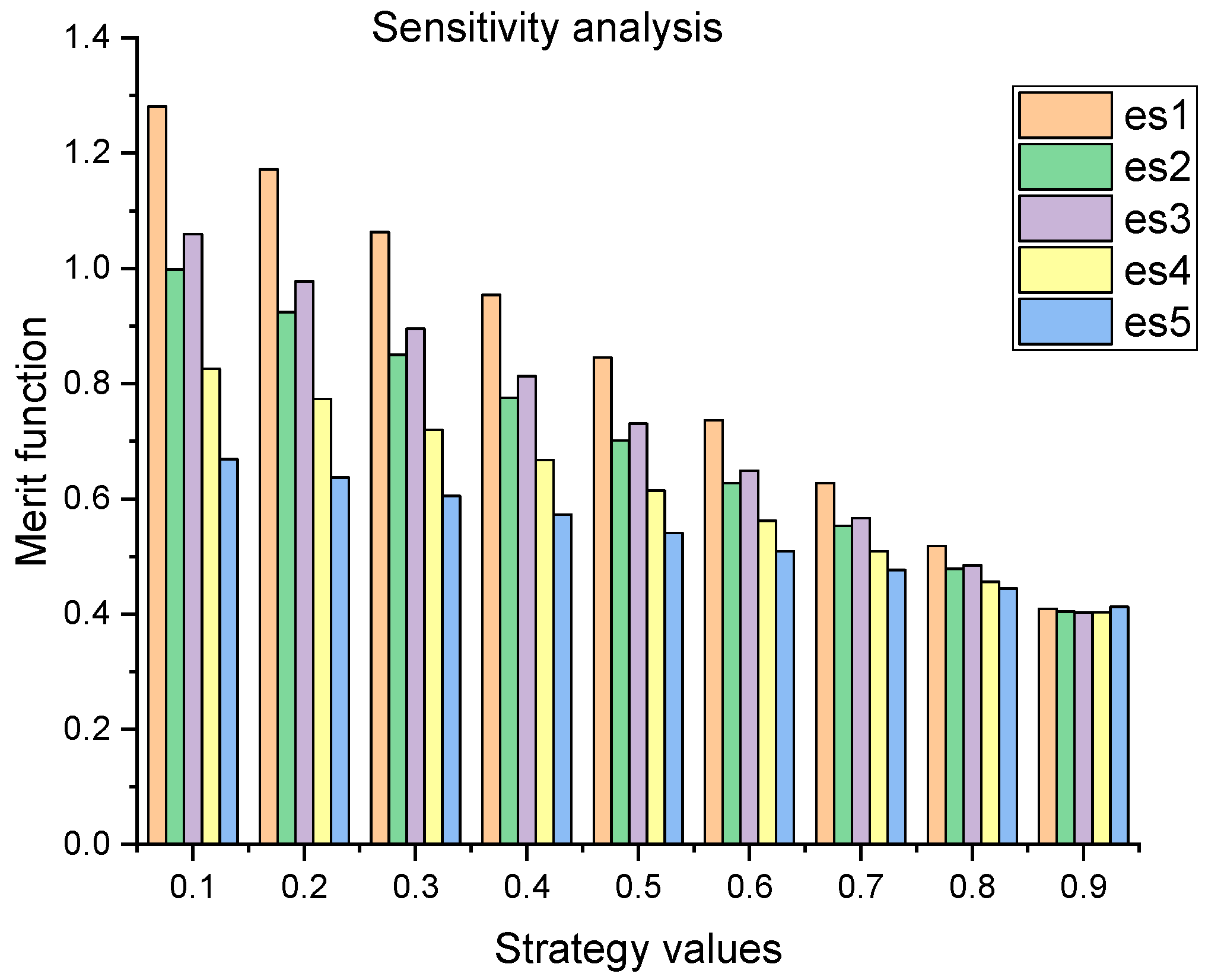
shows the parameter values for the extended COPRAS method under q-ROFS context. At $v=0.50$, the final ranking order is calculated, and it is given by $e{s}_1>e{s}_3>e{s}_2>e{s}_4>e{s}_5$. Figure 2 presents the sensitivity analysis of strategy values at regular step size from 0.10 to 0.90. From the analysis, we observe that the ranking order does not change, which concludes that the proposed framework is stable.

Step 7: Compare the performance of the proposed framework with other state-of-the-art methods by using the factors discussed in Section 5.

Table 6. Rank values from different methods.

Energy Sources	Methods
	[17]	[19]	[21]	[18]	Proposed
$e{s}_1$	1	1	1	1	1
$e{s}_2$	3	2	3	2	3
$e{s}_3$	2	3	2	3	2
$e{s}_4$	4	4	4	4	4
$e{s}_5$	5	5	5	5	5

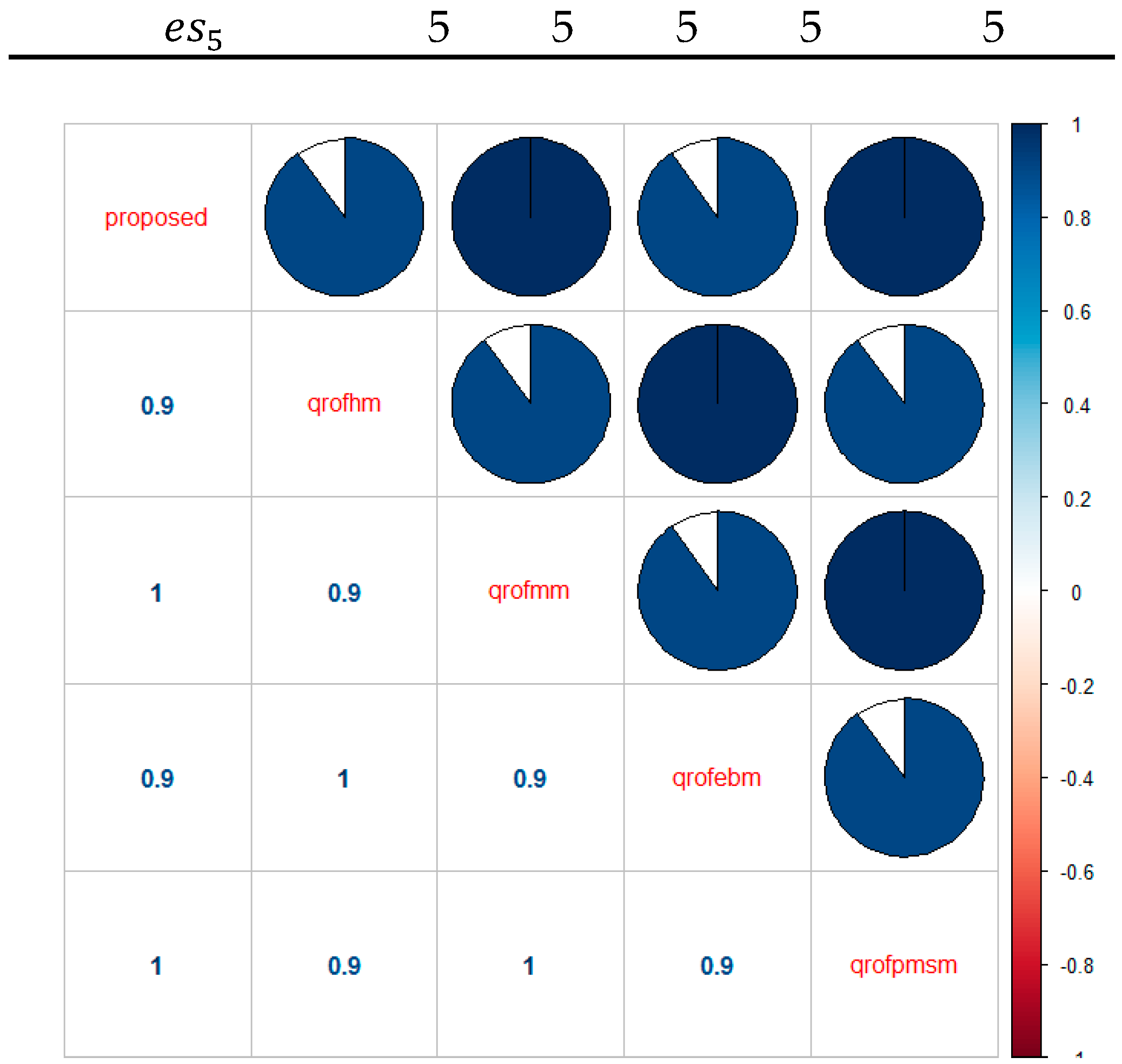
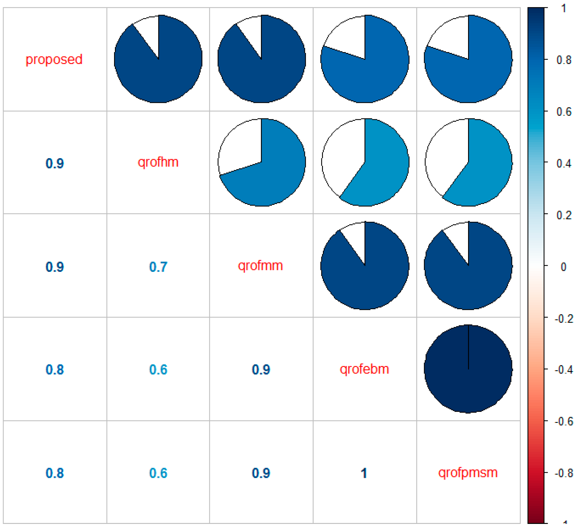
shows the ranking order obtained from different ranking methods, which are given as input to the Spearman correlation [53] for understanding the consistency of the proposed framework. Four methods viz., Liu et al. method [17], Liu et al. [19] method, Wei et al. [18], and Wang et al. [21] are taken for comparison with the view of maintaining homogeneity. From Figure 3, we observe that the proposed framework is highly consistent with other methods.

Step 8: End.

Example 2.

Renewable energy source selection.

This is another example that demonstrates the practical use of the proposed framework by selecting a suitable energy source from the set of sources based on certain evaluation attributes. As mentioned above, the energy sources and the attributes for evaluation are kept unchanged. The DMs adopt q-ROFNs for preference elicitation and the procedure for selection of a suitable renewable energy source is provided below:

Step 1: Begin.

Step 2: Construct three decision matrices of order $5\times 6$ as of Example 1. q-ROFN is used as preference information. The renewable energy sources and the evaluation attributes are kept unchanged.

Table 7. Preference information from each DM and aggregated preference information.

Energy Sources	Attributes
	${\mathit{z}}_1$	${\mathit{z}}_2$	${\mathit{z}}_3$	${\mathit{z}}_4$	${\mathit{z}}_5$	${\mathit{z}}_6$
$d_1$
$e{s}_1$	(0.36,0.70)	(0.86,0.51)	(0.13,0.32)	(0.10,0.41)	(0.69,0.13)	(0.32,0.68)
$e{s}_2$	(0.79,0.18)	(0.16,0.14)	(0.48,0.22)	(0.87,0.58)	(0.42,0.76)	(0.12,0.32)
$e{s}_3$	(0.18,0.86)	(0.32,0.64)	(0.50,0.88)	(0.46,0.77)	(0.25,0.48)	(0.16,0.70)
$e{s}_4$	(0.85,0.29)	(0.28,0.61)	(0.18,0.78)	(0.57,0.42)	(0.23,0.21)	(0.38,0.43)
$e{s}_5$	(0.30,0.61)	(0.58,0.87)	(0.14,0.45)	(0.12,0.33)	(0.27,0.37)	(0.56,0.78)
$d_2$
$e{s}_1$	(0.42,0.78)	(0.15,0.46)	(0.20,0.69)	(0.28,0.76)	(0.75,0.23)	(0.11,0.13)
$e{s}_2$	(0.43,0.54)	(0.36,0.64)	(0.39,0.84)	(0.55,0.17)	(0.52,0.57)	(0.72,0.23)
$e{s}_3$	(0.60,0.28)	(0.27,0.48)	(0.68,0.86)	(0.24,0.13)	(0.25,0.76)	(0.75,0.79)
$e{s}_4$	(0.13,0.31)	(0.67,0.76)	(0.69,0.38)	(0.51,0.51)	(0.47,0.51)	(0.45,0.39)
$e{s}_5$	(0.56,0.42)	(0.52,0.63)	(0.64,0.56)	(0.36,0.77)	(0.18,0.86)	(0.72,0.64)
$d_3$
$e{s}_1$	(0.38,0.73)	(0.50,0.81)	(0.42,0.13)	(0.60,0.45)	(0.42,0.69)	(0.19,0.68)
$e{s}_2$	(0.21,0.67)	(0.25,0.15)	(0.61,0.38)	(0.38,0.35)	(0.17,0.12)	(0.21,0.79)
$e{s}_3$	(0.39,0.47)	(0.71,0.35)	(0.56,0.48)	(0.72,0.86)	(0.57,0.16)	(0.51,0.60)
$e{s}_4$	(0.35,0.19)	(0.81,0.70)	(0.59,0.84)	(0.61,0.12)	(0.79,0.14)	(0.46,0.67)
$e{s}_5$	(0.19,0.13)	(0.57,0.34)	(0.47,0.28)	(0.76,0.73)	(0.44,0.20)	(0.64,0.31)
Aggregated Matrix
$e{s}_1$	(0.39,0.83)	(0.77,0.87)	(0.37,0.39)	(0.53,0.65)	(0.69,0.80)	(0.28,0.79)
$e{s}_2$	(0.71,0.78)	(0.31,0.42)	(0.55,0.60)	(0.78,0.58)	(0.46,0.39)	(0.63,0.86)
$e{s}_3$	(0.53,0.66)	(0.63,0.58)	(0.61,0.66)	(0.64,0.90)	(0.50,0.43)	(0.66,0.74)
$e{s}_4$	(0.76,0.45)	(0.73,0.80)	(0.62,0.89)	(0.58,0.39)	(0.71,0.41)	(0.44,0.79)
$e{s}_5$	(0.49,0.39)	(0.56,0.57)	(0.57,0.53)	(0.68,0.82)	(0.39,0.46)	(0.66,0.56)

provides the preference information from different DMs.

Step 3: These matrices are aggregated by using newly proposed q-ROFGMSM operator and it is shown in Table 7. The DMs’ weights are adapted from Example 1.

The risk appetite values are given by ${\lambda }_1=2$ and ${\lambda }_2=1$. The weight of each DM is adapted from Example 1 and Table 7 presents the input information and the aggregated matrix obtained by applying Equation (16). From Table 7, it is inferred that the order of the aggregated matrix remains unchanged as that of the input.

Step 4: Attributes’ weights are also adapted from Example 1. By using the aggregated matrix (from Step 3) and the attribute weight vector (from Example 1), renewable energy sources are prioritized by using proposed q-ROFS based COPRAS method. The sensitivity analysis is performed over strategy values to realize its effect on prioritization order.

The attributes’ weights are adapted from Example 1 and

Table 8. Parameters of complex proportional assessment (COPRAS) ranking method under q-ROFS context.

Energy Sources	Parameters
	${\mathit{P}}_{\mathit{i}}$	${\mathit{R}}_{\mathit{i}}$	$\mathit{T}{\mathit{R}}_{\mathit{i}}\left(0.5\right)$
$e{s}_1$	(0.57,0.01)	(0.34,0.25)	0.91
$e{s}_2$	(0.60,0.00)	(0.34,0.04)	0.86
$e{s}_3$	(0.57,0.01)	(0.36,0.03)	0.8
$e{s}_4$	(0.64,0.00)	(0.37,0.03)	0.77
$e{s}_5$	(0.55,0.00)	(0.34,0.02)	0.66

presents the COPRAS parameter values. From Table 8, the prioritization order is given by $e{s}_1>e{s}_2>e{s}_3>e{s}_4>e{s}_5$. Thus, tidal energy is chosen as a suitable source among the set of renewable energy sources.

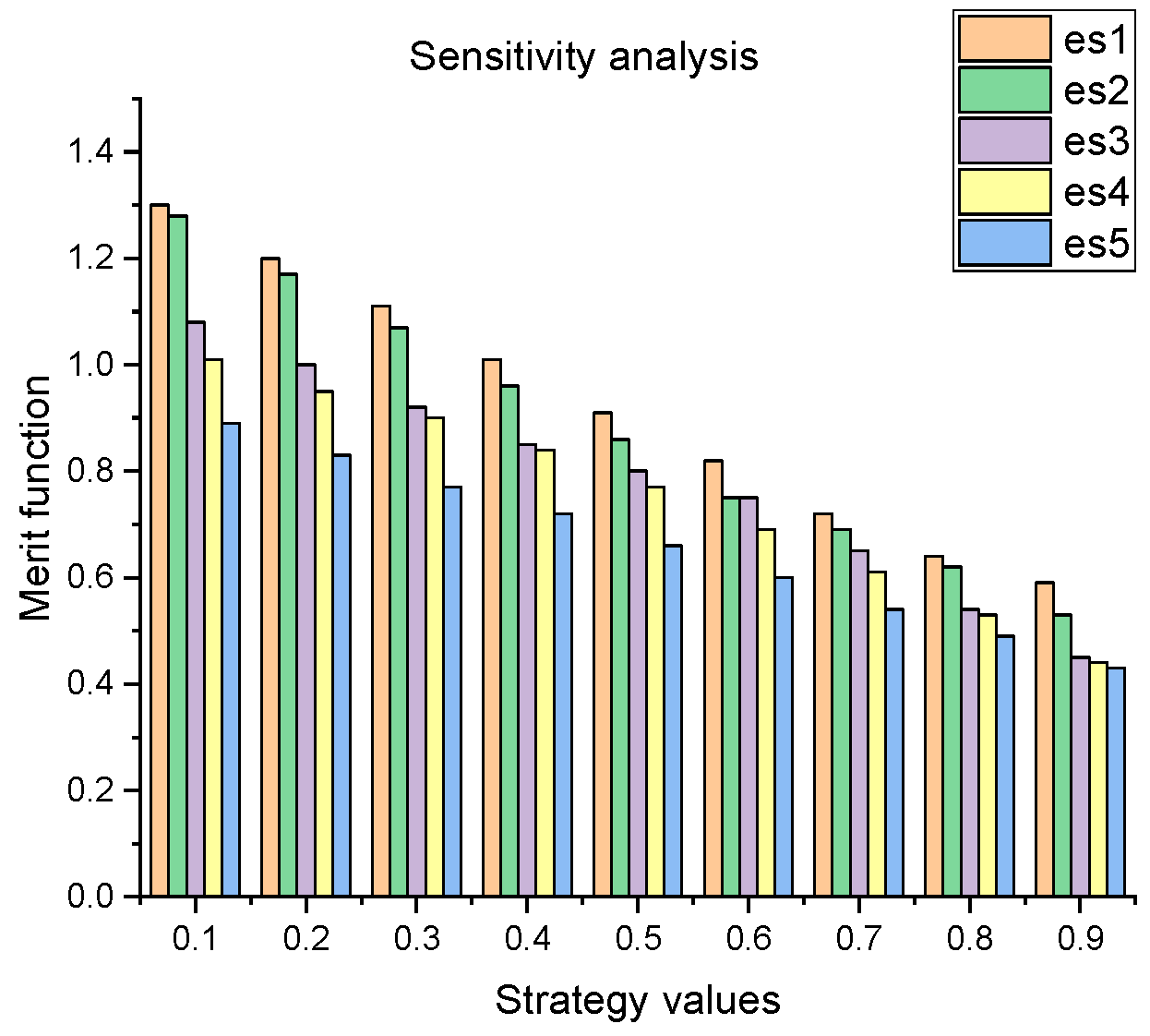
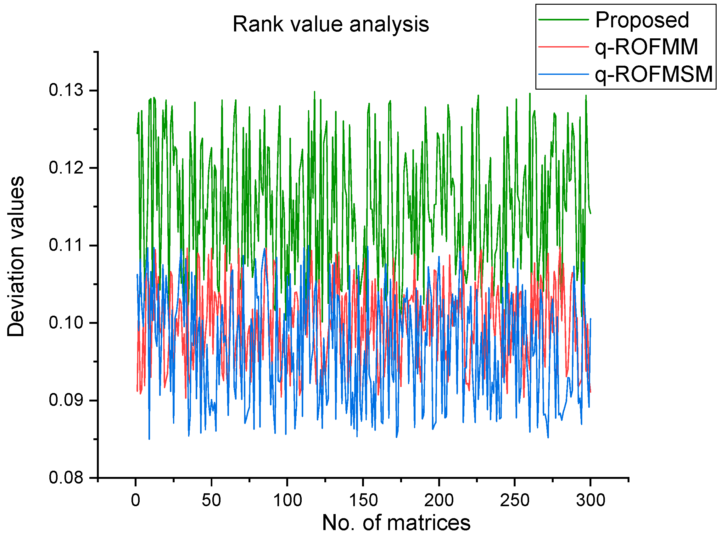
Table 8 shows the merit function at $v=0.50$. To further understand the effects of different strategy values on the prioritization order, sensitivity analysis test is performed. The strategy values are varied in a step wise manner from 0.1 to 0.9 and its effect on the merit function is presented in Figure 4. The physical meaning of strategy value is provided in Example 1 for clarity. From Figure 4, it is observed that the proposed framework is unaffected by the adequate changes to strategy values and is robust in nature.

Step 5: Finally, the consistency of the proposed framework is analyzed by comparison with other methods using Spearman correlation.

From

Table 9. Prioritization order from different methods.

Energy Sources	Methods
	[17]	[19]	[21]	[18]	Proposed
$e{s}_1$	2	1	1	1	1
$e{s}_2$	1	3	3	3	2
$e{s}_3$	3	2	2	2	3
$e{s}_4$	4	4	5	5	4
$e{s}_5$	5	5	4	4	5

and Figure 5, it is clear that the proposed framework produces unique prioritization order for the provided preference information. Based on the majority wins principle, tidal energy $e{s}_1$ is a suitable source and the reason for unique prioritization order in this situation can be intuitively understood from the fact that the proposed framework mitigates human intervention and information loss by retained the q-rung orthopair fuzzy nature. From Figure 5, the proposed framework is consistent with other state-of-the-art methods.

Step 6: End.

5. Comparative Investigation of Proposed Decision Framework

This section provides a comparative investigation of the proposed framework with other state-of-the-art methods under both theoretical and numerical factors. Proposed decision framework is compared with four methods mentioned above under both theoretical and numerical contexts.

Table 10. Characteristics of different methods.

Context	Methods
	Proposed	[17]	[19]	[21]	[18]
Data	q-ROFS based preference information
Operator	GMSM	Power MSM	Extended Bonferroni mean	Muirhead mean	Heronian mean
DMs’ weights	Calculated systematically	Directly provided
Attributes’ weights	Calculated systematically	Provided directly	Entropy method	Provided directly
Interrelationships	yes, among attributes	yes, among attributes	yes, between attributes	yes, among attributes	yes, between attributes
Prioritization method	Extended COPRAS	no
Nature of information	Partial information on each DM and attribute is known	n/a
Complexity	$O\left(dmn+dn+dmn+mn\right)=O(2dmn+n\left(d+m\right)$ where d is the number of DMs, m is the number of energy sources, and n is the number of evaluation attributes	$O\left(dmn+mn\right)=O\left(mn\left(d+1\right)\right)$
Efficiency	Though the proposed framework is complex compared to its counterparts, (i) it is highly systematic and produces rational decision-making; (ii) reduces human intervention effectively; and (iii) produces consistent, robust, and broad prioritization of energy sources.	The aggregation operator and the ranking method extended from the operator are specific cases of proposed framework. Morrover, human intervention is high compared to proposed framework.
Easiness	Proposed framework is complicated in the short run, but in the long run, the methods are highly systematic and produce rational decision with fewer inaccuracies (caused by human intervention) and proper justification.	Though these methods appear easy in the short run, they involve human intervention which causes inaccuracies in decision-making. Parameters like DMs‘ weights and attributes‘ weights are not calculated in a systematic manner.

presents a comparative investigation.

The following are the strengths of the proposed framework analyzed from Table 10:

• Uncertainty and vagueness are handled effectively by using a generalized preference style viz., q-ROFS. This allows DMs to flexibly provide their membership and non-membership values over a specific instance;
• Preferences are aggregated rationally by properly capturing the interrelationship among attributes. Moreover, the DMs’ weights are calculated in a systematic manner for proper aggregation of information;
• Further, attributes’ weights are calculated rationally by making use of the partially known information about each attribute;
• Energy sources are prioritized by considering the nature of the attributes (extended COPRAS method under q-ROFS);
• The proposed framework is highly consistent with other state-of-the-art methods which can be observed from Figure 3;
• Furthermore, the framework is stable even after strategy values are changed at regular step size. It can be observed from Figure 2;
• The broadness of rank values is also an important strength of the proposed decision framework. To realize the same, 300 matrices of order $5\times 6$ are considered as input for the framework and rank values are determined for each matrix. The deviation is calculated for each vector (rank value), and they are depicted in Figure 6. From the analysis, it is inferred that the proposed framework produces a broad rank value set compared to other state-of-the-art methods.

The weaknesses of the framework are as follows:

• Optimal selection of risk appetite values for each DM during the process of aggregation is complex;
• Furthermore, DMs must be trained with the preference style for effective elicitation of preferences. Though the window for preference elicitation is wider compared to its counterparts, DMs must be trained for better elicitation of preferences.

The weaknesses of the framework are as follows:

3.

Optimal selection of risk appetite values for each DM during the process of aggregation is complex;

4.

Furthermore, DMs must be trained with the preference style for effective elicitation of preferences.

6. Conclusions

This paper provides a new decision framework under q-ROFS context for rational selection of renewable energy sources under the Indian perspective. The framework presents a new extension to the GMSM operator by calculating weights of DMs in a systematic manner when partial information is known. Moreover, attributes’ weights are also calculated under the same context. Further, prioritization of energy sources is done by using an extended COPRAS method under q-ROFS. The stability of the framework is realized by a sensitivity analysis of strategy values. Furthermore, consistency is discussed by using the Spearman correlation. The broadness of the rank value set is realized by using simulation analysis.

Some managerial implications are:

• The proposed framework is readily available for the rational selection of energy sources. However, the same framework is flexible for other MAGDM problems as well;
• Uncertainty is handled effectively by using q-ROFS, which is a generalized form that provides a wider window for preference elicitation;
• The framework can be used for effective energy planning and can help people to gain awareness of the urge for renewable energy alternatives.

As a future direction to the research, new decision frameworks are planned for rational selection of renewable energy sources under linguistic context, and energy utilization schemes can be developed for sustainable growth of the nation. Situations where both the DMs’ weights and attributes’ weights are unknown can also be addressed under the context of q-ROFS based MAGDM problems.

References

1. Indragandhi, V.; Subramaniyaswamy, V.; Logesh, R. Resources, configurations, and soft computing techniques for power management and control of PV/wind hybrid system. Renew. Sustain. Energy Rev. 2016, 69, 129–143. [Google Scholar]
2. Pillai, I.R.; Banerjee, R. Renewable energy in India: Status and potential. Energy 2009, 34, 970–980. [Google Scholar] [CrossRef]
3. Reddy, S.; Painuly, J.P. Diffusion of renewable energy technologies-barriers and stakeholders’ perspectives. Renew. Energy 2004, 29, 1431–1447. [Google Scholar] [CrossRef]
4. Mardani, A.; Zavadskas, E.K.; Khalifah, Z.; Zakuan, N.; Jusoh, A.; Nor, K.M.; Khoshnoudi, M. A review of multi-criteria decision-making applications to solve energy management problems: Two decades from 1995 to 2015. Renew. Sustain. Energy Rev. 2017, 71, 216–256. [Google Scholar] [CrossRef]
5. Chatterjee, K.; Kar, S. A multi-criteria decision making for renewable energy selection using Z-Numbers. Technol. Econ. Dev. Econ. 2018, 24, 739–764. [Google Scholar] [CrossRef]
6. Baek, S.; Lee, B. Optimal Decision-Making of Renewable Energy Systems in Buildings in the Early Design Stage. Sustainability 2019, 11, 1471. [Google Scholar] [CrossRef]
7. González, A.M.; Sandoval, H.; Acosta, P.; Henao, F. On the acceptance and sustainability of renewable energy projects-a systems thinking perspective. Sustainability 2016, 8, 1171. [Google Scholar] [CrossRef]
8. Cavallaro, F.; Zavadskas, E.K.; Streimikiene, D. Concentrated solar power (CSP) hybridized systems. Ranking based on an intuitionistic fuzzy multi-criteria algorithm. J. Clean. Prod. 2018, 179, 407–416. [Google Scholar] [CrossRef]
9. Cavallaro, F.; Zavadskas, E.K.; Streimikiene, D.; Mardani, A. Assessment of concentrated solar power (CSP) technologies based on a modified intuitionistic fuzzy topsis and trigonometric entropy weights. Technol. Forecast. Soc. Chang. 2019, 140, 258–270. [Google Scholar] [CrossRef]
10. Yager, R.R. Generalized Orthopair Fuzzy Sets. IEEE Trans. Fuzzy Syst. 2017, 25, 1222–1230. [Google Scholar] [CrossRef]
11. Atanassov, K.T. Intuitionistic fuzzy sets. Fuzzy Sets Syst. 1986, 20, 87–96. [Google Scholar] [CrossRef]
12. Yager, R.R. Pythagorean membership grades in multicriteria decision making. IEEE Trans. Fuzzy Syst. 2014, 22, 958–965. [Google Scholar] [CrossRef]
13. Yager, R.R.; Alajlan, N. Approximate reasoning with generalized orthopair fuzzy sets. Inf. Fusion 2017, 38, 65–73. [Google Scholar] [CrossRef]
14. Du, W.S. Minkowski-type distance measures for generalized orthopair fuzzy sets. Int. J. Intell. Syst. 2018, 33, 802–817. [Google Scholar] [CrossRef]
15. Li, L.; Zhang, R.; Wang, J.; Shang, X.; Bai, K. A novel approach to multi-attribute group decision-making with q-rung picture linguistic information. Symmetry 2018, 10, 172. [Google Scholar] [CrossRef]
16. Cường, B.C. Picture fuzzy sets. J. Comput. Sci. Cybern. 2015, 30, 409–420. [Google Scholar] [CrossRef]
17. Liu, P.; Chen, S.; Wang, P. Multiple-Attribute Group Decision-Making Based on q-Rung Orthopair Fuzzy Power Maclaurin Symmetric Mean Operators. IEEE Trans. Syst. Man Cybern. 2018, 1–16. [Google Scholar] [CrossRef]
18. Wei, G.; Gao, H.; Wei, Y. Some q-rung orthopair fuzzy Heronian mean operators in multiple attribute decision making. Int. J. Intell. Syst. 2018, 33, 1426–1458. [Google Scholar] [CrossRef]
19. Liu, Z.; Liu, P.; Liang, X. Multiple attribute decision-making method for dealing with heterogeneous relationship among attributes and unknown attribute weight information under q-rung orthopair fuzzy environment. Int. J. Intell. Syst. 2018, 33, 1900–1928. [Google Scholar] [CrossRef]
20. Bai, K.; Zhu, X.; Wang, J.; Zhang, R. Some Partitioned Maclaurin Symmetric Mean Based on q-Rung Orthopair Fuzzy Information for Dealing with Multi-Attribute Group Decision Making. Symmetry 2018, 10, 383. [Google Scholar] [CrossRef]
21. Wang, J.; Zhang, R.; Zhu, X.; Zhou, Z.; Shang, X.; Li, W. Some q-rung orthopair fuzzy Muirhead means with their application to multi-attribute group decision-making. J. Intell. Fuzzy Syst. 2019, 36, 1599–1614. [Google Scholar] [CrossRef]
22. Koksalmis, E.; Kabak, Ö. Deriving Decision Makers’ Weights in Group Decision Making: An Overview of Objective Methods. Inf. Fusion 2019, 49, 146–160. [Google Scholar] [CrossRef]
23. Mousavi-Nasab, S.H.; Sotoudeh-Anvari, A. A comprehensive MCDM-based approach using TOPSIS, COPRAS and DEA as an auxiliary tool for material selection problems. Mater. Des. 2017, 121, 237–253. [Google Scholar] [CrossRef]
24. Saaty, T.L. Decision making with the analytic hierarchy process. Int. J. Serv. Sci. 2008, 1, 83–98. [Google Scholar] [CrossRef]
25. Rouyendegh, B.D. Developing an integrated AHP and Intuitionistic Fuzzy TOPSIS methodology. Tech. Gaz. 2014, 21, 1313–1320. [Google Scholar]
26. Xia, M.; Xu, Z. Entropy/cross entropy-based group decision making under intuitionistic fuzzy environment. Inf. Fusion 2012, 13, 31–47. [Google Scholar] [CrossRef]
27. Wood, D.A. Supplier selection for development of petroleum industry facilities, applying multi-criteria decision making techniques including fuzzy and intuitionistic fuzzy TOPSIS with flexible entropy weighting. J. Nat. Gas Sci. Eng. 2016, 28, 594–612. [Google Scholar] [CrossRef]
28. Wang, B.; Liang, J.; Qian, Y. Determining decision makers’ weights in group ranking: A granular computing method. Int. J. Mach. Learn. Cybern. 2015, 6, 511–521. [Google Scholar] [CrossRef]
29. Maclaurin, C. A fecond Letter to martin folkes, esq., concerning the roots of equations with demonstration of other roots of algebra. Philos. Trans. R. Soc. Lond. Ser. A 1729, 36, 59–96. [Google Scholar]
30. Zavadskas, E.K.; Kaklauskas, A.; Sarka, V. The new method of multicriteria complex proportional assessment of projects. Technol. Econ. Dev. Econ. 1994, 1, 131–139. [Google Scholar]
31. Zavadskas, E.K.; Kaklauskas, A.; Turskis, Z.; Tamošaitiene, J. Selection of the effective dwelling house walls by applying attributes values determined at intervals. J. Civ. Eng. Manag. 2008, 14, 85–93. [Google Scholar] [CrossRef]
32. Zavadskas, E.K.; Turskis, Z.; Kildienė, S. State of art surveys of overviews on MCDM/MADM methods. Technol. Econ. Dev. Econ. 2014, 20, 165–179. [Google Scholar] [CrossRef]
33. Mondal, S.; Kuila, S.; Singh, A.K.; Chatterjee, P.A. Complex Proportional Assessment Method-Based Framework for Industrial Robot. Int. J. Res. Sci. Eng. 2017, 3, 368–378. [Google Scholar]
34. Vahdani, B.; Mousavi, S.M.; Tavakkoli-Moghaddam, R.; Ghodratnama, A.; Mohammadi, M. Robot selection by a multiple criteria complex proportional assessment method under an interval-valued fuzzy environment. Int. J. Adv. Manuf. Technol. 2014, 73, 687–697. [Google Scholar] [CrossRef]
35. Gorabe, D.; Pawar, D.; Pawar, N. Selection of Industrial Robots using Complex Proportional Assessment Method. Am. Int. J. Res. Sci. Technol. Eng. Math. Sci. Technol. Eng. Math. 2014, 5, 140–143. [Google Scholar]
36. Zavadskas, E.K.; Turskis, Z.; Tamošaitiene, J.; Marina, V. Multicriteria selection of project managers by applying grey criteria. Technol. Econ. Dev. Econ. 2008, 14, 462–477. [Google Scholar] [CrossRef]
37. Zavadskas, E.K.; Kaklauskas, A.; Turskis, Z.; Tamošaitienė, J. Multi-Attribute Decision-Making Model by Applying Grey Numbers. Informatica 2009, 20, 305–320. [Google Scholar]
38. Hajiagha, S.H.R.; Hashemi, S.S.; Zavadskas, E.K. A complex proportional assessment method for group decision making in an interval-valued intuitionistic fuzzy environment. Technol. Econ. Dev. Econ. 2013, 19, 22–37. [Google Scholar] [CrossRef]
39. Valipour, A.; Yahaya, N.; Md Noor, N.; Antuchevičienė, J.; Tamošaitienė, J. Hybrid SWARA-COPRAS method for risk assessment in deep foundation excavation project: An Iranian case study. J. Civ. Eng. Manag. 2017, 23, 524–532. [Google Scholar] [CrossRef]
40. Mardani, A.; Jusoh, A.; Halicka, K.; Ejdys, J.; Magruk, A.; Ungku, U.N. Determining the utility in management by using multi-criteria decision support tools: A review. Econ. Res. Ekon. Istraz. 2018, 31, 1666–1716. [Google Scholar] [CrossRef]
41. Stefano, N.M.; Casarotto Filho, N.; Garcia Lupi Vergara, L.; Garbin Da Rocha, R.U. COPRAS (Complex Proportional Assessment): State of the art research and its applications. IEEE Lat. Am. Trans. 2015, 13, 3899–3906. [Google Scholar] [CrossRef]
42. Bielinskas, V.; Burinskienė, M.; Podviezko, A. Choice of abandoned territories conversion scenario according to MCDA methods. J. Civ. Eng. Manag. 2018, 24, 79–92. [Google Scholar] [CrossRef]
43. Wang, L.E.; Liu, H.C.; Quan, M.Y. Evaluating the risk of failure modes with a hybrid MCDM model under interval-valued intuitionistic fuzzy environments. Comput. Ind. Eng. 2016, 102, 175–185. [Google Scholar] [CrossRef]
44. Bausys, R.; Zavadskas, E.K.; Kaklauskas, A. Application of neutrosophic set to multicriteria decision making by COPRAS. Econ. Comput. Econ. Cybern. Stud. Res. 2015, 49, 91–105. [Google Scholar]
45. Roy, J.; Sharma, H.K.; Kar, S.; Zavadskas, E.K.; Saparauskas, J. An extended COPRAS model for multi-criteria decision-making problems and its application in web-based hotel evaluation and selection. Econ. Res. Ekon. Istraz. 2019, 32, 219–253. [Google Scholar] [CrossRef] [Green Version]
46. Ayrim, Y.; Atalay, K.D.; Can, G.E. A New Stochastic MCDM Approach Based on Copras. Int. J. Inf. Technol. Decis. Mak. 2018, 17, 857–882. [Google Scholar] [CrossRef]
47. Yazdani, M.; Chatterjee, P.; Zavadskas, E.K.; Hashemkhani Zolfani, S. Integrated QFD-MCDM framework for green supplier selection. J. Clean. Prod. 2017, 142, 3728–3740. [Google Scholar] [CrossRef]
48. Chatterjee, P.; Athawale, V.M.; Chakraborty, S. Materials selection using complex proportional assessment and evaluation of mixed data methods. Mater. Des. 2011, 32, 851–860. [Google Scholar] [CrossRef]
49. Chatterjee, P.; Chakraborty, S. Material selection using preferential ranking methods. Mater. Des. 2012, 35, 384–393. [Google Scholar] [CrossRef]
50. Zheng, Y.; Xu, Z.; He, Y.; Liao, H. Severity assessment of chronic obstructive pulmonary disease based on hesitant fuzzy linguistic COPRAS method. Appl. Soft Comput. J. 2018, 69, 60–71. [Google Scholar] [CrossRef]
51. Chatterjee, K.; Kar, S. Supplier selection in Telecom supply chain management: A Fuzzy-Rasch based COPRAS-G method. Technol. Econ. Dev. Econ. 2018, 24, 765–791. [Google Scholar] [CrossRef]
52. Luthra, S.; Kumar, S.; Garg, D.; Haleem, A. Barriers to renewable/sustainable energy technologies adoption: Indian perspective. Renew. Sustain. Energy Rev. 2015, 41, 762–776. [Google Scholar] [CrossRef]
53. Spearman, C. The Proof and Measurement of Association between Two Things. Am. J. Psychol. 1904, 15, 72–101. [Google Scholar] [CrossRef]
Figure 1. Proposed q-rung orthopair fuzzy set (q-ROFS) based decision framework with partially known weights.
Sustainability 11 04202 g001
Figure 2. Sensitivity analysis: Strategy values of DMs.
Sustainability 11 04202 g002
Figure 3. Corrplot of Spearman correlation from different ranking methods: Example 1.
Sustainability 11 04202 g003
Figure 4. Sensitivity analysis test on strategy values.
Sustainability 11 04202 g004
Figure 5. Corrplot of Spearman correlation from different ranking methods: Example 2.
Sustainability 11 04202 g005
Figure 6. Analysis of the broadness of rank values: Proposed vs. Others.
Sustainability 11 04202 g006