The Synergy of Financial Volatility between China and the United States and the Risk Conduction Paths

Abstract

Based on monthly data of six major financial variables from January 1996 to December 2018, this paper employs a structural vector autoregressive model to synthesize financial conditions indices in China and the United States, investigates fluctuation characteristics and the synergy of financial volatility using a Markov regime switching model, and further analyzes the transmission paths of the financial risk by using threshold regression. The results show that there is an approximately three-year cycle in the financial fluctuations of both China and the United States, and such fluctuations have a distinct asymmetry. Two thresholds were applied (i.e., 0.361 and 0.583), taking the synergy index (SI) as the threshold variable. The impact of the trade factor is significant across all thresholds and is the basis of financial linkages. When the SI is less than 0.361, the exchange rate factor is the main cause of the financial cycle comovement change. As the financial volatility synergy increases, the asset factor and interest rate factor start to become the primary causes. When the level of synergy breaks through 0.583, the capital factor based on stock prices and house price is still the main path of financial market linkage and risk transmission, but the linkage of monetary policy shows a restraining effect on synergy. Therefore, it is necessary to monitor the financial cycle and pay attention to the coordination between countries in terms of policy regulation.

1. Introduction

In the context of rapid economic growth and stable inflation, both Japan in 1990 and the United States in 2007 experienced large-scale capital market crashes. Severe credit contraction and shrinking asset prices triggered a long-term recession. The two crises made academics and policymakers aware that it is not sufficient to maintain economic sustainability without paying attention to financial market volatility [1,2]. The history of financial crises shows that most occur near the peak of the financial cycle. Moreover, the correlation between economic cycle and financial volatility is becoming closer. A financial crisis is often accompanied by a recession, and the financial expansion period often leads to credit expansion and is accompanied by economic recovery [3]. However, the traditional cycle theory based on the real business cycle fails to adequately consider the risk perception of banks and the cycle of asset prices. Therefore, it is difficult to reasonably explain the cyclical fluctuations of financial markets and to accurately capture the financial cycle changes [4].

Having reflected on the global financial crisis, Borio [5] proposed the concept of the “financial cycle”. The financial cycle is the result of the interaction between financial conditions such as credit constraints and the value of financial assets. The credit growth and real estate prices are the main elements, which can link the financial and real economy through channels such as balance sheets, leading to procyclical fluctuations in finance. When the economic cycle and financial cycle are superimposed simultaneously, the magnitude of economic expansion or contraction will be enlarged. When the economic cycle and the financial cycle are not synchronized, the direction of their roles may be different or even opposite. If those in charge of policymaking are not aware of the importance of risk appetite, credit constraints, and asset prices to the macroeconomy, and ignore the financial cycle, the regulatory policies implemented to curb the real economy recession are likely to cause risks related to financial imbalances. The theory of the financial cycle has become a new paradigm that is designed to fit the cyclical fluctuations of the macroeconomy under the modern financial system.

Driven by recent economic globalization and financial integration, the correlation between the real economy and the financial environment among countries has increased significantly. Especially during the outbreak of the US financial crisis, financial risks spread rapidly among financial markets in various countries, which eventually led to a global economic recession. Therefore, on the basis of analyzing and testing the fluctuation situation and the operation characteristics of the financial cycle, it is necessary to further explore the law of synergy among the financial cycles of various countries, which will help countries to carry out international measures of cooperation in financial relations and real economic regulation.

China, a developing country with the fastest economic growth rate in the world, and the United States, a developed country with the largest economy in the world, have played a vital role in global financial and economic development in recent years. According to World Bank data [6], the contribution rate of major countries and regions to world economic growth from 2012 to 2016 is 10% in the United States and 34% in China. The financial and economic relationship between China and the United States not only helps to encourage the stable and healthy development of the economies of both countries, but also has a guiding and transmitting role that cannot be ignored for the economic and financial market stability of other countries. In the event that the internal economic or financial markets of China and the United States are out of balance, imbalance within the world economy is inevitable. Therefore, studying the characteristics related to volatility within the financial cycle observed between China and the United States, as well as its coordination mechanism, can not only provide useful empirical evidence and policy implications for the reform and development of China’s financial system, but can also be of significant value in terms of maintaining global financial stability and economic sustainability.

This paper aims to analyze the synchronization between the financial cycles of China and the United States, and discuss its transmission path. Specifically, this paper selects six types of financial indicators, including the interest rate, credit, money supply, house price, stock price, and exchange rate for the period January 1996 to December 2018 in China and the United States, in order to synthesize the financial conditions index (FCI), the fluctuations can be used to measure the financial cycle. The weights of the financial indicators used in the FCI are determined by the structural vector autoregressive (SVAR) model and the impulse response function (IRF). The Markov regime switching model is then used to identify the turning points of the respective FCI series of the two countries to complete the division of the cycle. Furthermore, we use the rolling consistency index and correlation coefficient to measure the synergy of financial cycles between China and the United States. Finally, considering that there may be differences in the factors affecting the synergy of financial cycles between China and the United States in different periods, threshold regression is used to empirically analyze the factors affecting the synergy.

The structure of the paper is as follows: Section 2 presents a literature review; Section 3 describes the dataset, variables, and methods used; Section 4 presents the main results, and Section 5 discusses the conduction path of financial cycle synergy. Finally, Section 6 outlines some conclusions and observations.

2. Literature Review

The study of the financial cycle can be traced back to the debt–deflation theory proposed by Fisher [7] during the Great Depression, which argues that excessive debt and deflation will interact and spiral upward, causing a recession. However, the Keynesian economic cycle theory based on the IS (Investment-Saving equation)–LM (Liquidity preference-Money supply equation) framework was the main paradigm in the field of macroeconomic cycle research. The Keynesian school divided macroeconomics into short-term fluctuations and long-term growth trends. The short-term real economy volatility represented by real GDP is a deviation from the long-term potential GDP trend. The two oil crises and the lack of explanation for the stagflation led to a questioning of Keynesianism by the neoclassical macroeconomics advocated by Lucas [8]. After the 1980s, the real business cycle theory that used exogenous practical factors to explain the root causes of economic cycle fluctuations became the core of neoclassical macroeconomic theory [9,10]. However, both the Keynesian economic cycle theory and the real economic cycle theory (hereinafter referred to as the “traditional economic cycle theory”) ignore the role of financial friction in the macroeconomy. The outbreak of the global financial crisis in 2007 exposed the shortcomings of traditional economic cycle theory, which focuses only on the fluctuation of the real economy, but sets up the financial market too simply [11], resulting in a disconnection from real macroeconomic development.

The profound lessons of the global financial crisis have led economists to realize that mature economies are likely to be swallowed up overnight by seemingly prosperous financial illusions, with greater damage and longer recovery periods [5]. Bernanke et al. [12] revised the premise of financial neutrality theory, and the important role of financial factors in the economic cycle was established. Subsequently, a large number of studies have shown that the volatility of the financial system not only delays the natural regression of the macroeconomy to its stable state, but may also generate an accelerator effect or procyclical effect, which amplifies the fluctuation of the real economy [13,14,15,16]. The measurement of the financial cycle and related research then began to appear and continued to increase [16,17,18]. Based on these empirical findings, Borio [5] formally proposed the concept of financial cycles in 2014.

Comparable to the traditional economic cycle, there are also medium- and long-term low-frequency fluctuation components and short-period high-frequency fluctuation components in the financial cycle fluctuations. The characterization of low-frequency fluctuations in the financial cycle is mostly concentrated on real estate prices or credit cycles [19,20,21]. The variation of these variables is dominated by low-frequency fluctuations, and their wavelengths and amplitudes are larger than the traditional economic cycle. Due to the strong correlation between these variables and the macroeconomy in the medium and long term, the financial cycle measured by these variables is usually accompanied by a financial crisis after the peak. Therefore, the monitoring of such low-frequency fluctuations tends to identify the risk of future financial distress or financial crisis in advance.

The research on high-frequency fluctuations of the financial cycle mainly extends consideration to other financial variables, such as stock price, money supply, interest rate, and exchange rate, and constructs the financial conditions index (FCI) [22] by combining multiple financial variables or extracting common components from them using statistical methods to investigate the cyclical changes of the overall financial environment [23,24]. This type of research not only introduces high-frequency financial variables, but also takes into account the fluctuations of financial variables in different fields, so the length of the financial cycle is generally consistent with or even shorter than that of the macroeconomic cycle.

The high-frequency volatility component of the financial cycle reflects the interaction between financial factors and the macroeconomy. It not only reveals the volatility of the financial market under various internal and external shocks, but also reflects the dynamic response of monetary policy and other financial policies to the economic and financial environment. Therefore, considering that the purpose of this study is to analyze the synergy of financial volatility between China and the United States, we chose to develop an FCI with high-frequency factors to measure the financial cycle.

In recent years, the method of using multiple financial indicators to synthesize an FCI to measure the overall financial situation has been widely recognized by domestic and foreign academic circles. In fact, the financial stress index (FSI) [25,26] that reflects the risk pressure of the financial system is also widely used. However, the FCI can be used as a leading indicator to predict the future state of other macroeconomic indicators because it contains financial variables that reflect future economic and inflationary information. Compared with FSI, FCI is more macroscopic. This is consistent with the original intention of this paper—to study financial risk transmission to maintain economic growth and stability. Therefore, the paper chose to use FCI.

From the point of view of the existing literature, the calculation methods of the FCI are mainly divided into two types: extracting common components from various financial indicators and weighting of a combination of financial indicators. The former mainly uses principal component analysis, factor analysis, and a dynamic factor model [27,28] to extract the FCI index from multiple financial indicators. For example, Brave and Butters [29] used principal component analysis to extract the US FCI from a large number of financial indicators, and found that the calculated FCI can be used as an important basis for policy formulation and financial market evaluation. Matheson [30] used the dynamic factor model to synthesize the FCI of the United States and the European Union. The advantage of this method is that it captures more financial indicators and is not limited by specific theoretical assumptions, though it is disadvantageous as it ignores the correlation between financial indicators and macroeconomic target variables.

Thus, more scholars tend to determine weights according to the relationship between financial variables and macroeconomic target variables (such as inflation), and calculate the FCI by using a weighted combination of multiple financial indicators. There are roughly three kinds of methods to determine the weight of financial indicators using this type of calculation method. One method is to use the estimated values of coefficients in the large-scale macroeconomic simultaneous model as the basis for determining the weight of financial indicators. Dudley and Hatzius [31] estimated the impact of financial variables on gross domestic product (GDP) based on the large-scale macroeconomic model of the Federal Reserve, and used it as a weight to calculate the FCI of the United States. The second is to calculate the weight according to the estimated value of each financial variable coefficient in the simplified total demand equation. Montagnoli et al. [32] used this method to calculate the weights of various financial factors and synthesize the FCI in the United States, the United Kingdom, Canada, and the European Union. Wang [33] also used the same method to calculate China’s FCI. The third is to calculate the weight by using the cumulative impulse response of each financial variable to the target variable, such as inflation in the vector autoregressive (VAR) system. Swiston [34] calculated the US FCI by constructing a VAR model containing variables such as stock price, exchange rate, and loan standard, and found that it has a good predictive effect on economic growth. This method not only ensures the coverage of financial indicators, but is also advantageous as it is simple to calculate and is not dependent on the assumptions of economic theory, and thus has been the most widely used. Chinese scholars Feng et al. [35], Xu et al. [36], and Deng [37] also conducted a series of studies based on this method. This paper will also use the third method to calculate the FCI. Taking into account the contemporaneous correlation between variables, the pulse function of the structural vector autoregressive model is chosen to determine the weight of each financial indicator.

Although scholars have conducted substantial analyses of the financial situation of different countries based on the FCI, the methods of measuring FCI are different, and the financial indicators considered are also very different, which objectively hinders the study of financial cycles and their linkage in different countries. So far, the research on international financial relations, especially the characteristics of financial market linkages between China and the United States, is mostly limited to the independent analysis of specific financial markets or financial indicators. For example, Xiang et al. [38] studied the asymmetry of financial interdependence between China and the United States from three perspectives: bilateral capital dependence, bilateral capital flow structure, and bilateral capital cycle. Yu et al. [39] used the SVAR model to analyze the linkage between the currency market, the stock market, and the foreign exchange market in China and the United States. As an attempt and a supplement to the existing research, this paper intends to select six financial indicators, namely, real estate price, credit, stock price, money supply, interest rate, and exchange rate to measure their financial situation indices in a unified way. This study investigates the volatility characteristics and synergy of the financial cycle of the two countries, and further explores the influencing factors of international financial risk transmission under different levels of synergy. It is expected to provide an empirical framework and to highlight policy implications for maintaining the dual stability of China and the world’s real economy and virtual economy.

3. Indicators, Data, and Methods

3.1. Selection of Financial Indicators

In choosing and constructing the financial variables of the FCI, this paper follows two principles: one is that financial variables play an important role in the transmission mechanism of monetary policy; the other is that financial variables contain key information that can predict future macroeconomic conditions. According to this principle, and referring to relevant literature [40,41], the financial variables used to construct the FCI and the reasons for their selection are as follows:

Money Supply (MS) and Interest Rate (IR). As the main monetary policy tools of the central bank, money supply will indirectly and interest rate will directly affect the use cost of money, and then influence changes in the financial sub-markets, such as the stock market, through changes in the discount rate.

Credit Loans (CL). As a total index reflecting financial support to the real economy and financial and economic relations, total credit loans affect the economic behavior of enterprises and residents mainly by changing the financing conditions of financial markets and then influencing the economic and financial markets.

Exchange Rate (ER). Under the open economy, the effective exchange rate—as a weighted average exchange rate weighted by the proportion of foreign trade—is not only a bridge between one country’s currency and other countries’ currencies, but also an important link between the two countries’ prices. Its changes will affect a country’s economic and financial situation by causing changes in the trade balance, capital flows, and asset prices such as stock prices.

Share Prices (SP). Aside from foreign exchange assets and monetary assets, the composition of residents’ assets increasingly encompasses other assets, such as stocks and real estate. The change in the stock price index is not only related to the capital cost of a company, but also affects the family’s financial and consumption situation through various channels, such as the wealth effect, so it is one of the important financial indicators.

House Prices (HP). As financial assets include property, real estate is an important component of residents’ investment portfolio. Furthermore, real estate is often associated with credit expansion. The rapid rise of housing prices has greatly increased financial risks, although it can increase total consumption through the “wealth effect” and stimulate investment in related industries, such as cement and steel, to promote economic growth. Therefore, it is also a factor that must be taken into account in measuring the financial market situation.

3.2. Description and Processing of Data

The monthly data relates to 276 months from January 1996 to December 2018, which are selected as samples. If there are no special instructions, all of the data are derived from the CEInet Statistics Database [42]. The database is a comprehensive economic database group. According to its content and frequency, it is divided into nine sub-databases: China’s macro-monthly database, China’s macro-annual database, China’s provincial macro-annual database, China’s Customs monthly database, China’s County annual database, China’s urban annual database, the OECD (Organization for Economic Co-operation and Development) monthly database and the OECD annual database, covering the macroeconomy, industrial economy, regional economy, and world economy. All of the data in the database were obtained from various statistical and publishing departments, with stable, reliable, and authoritative sources.

The indicators used to describe China’s financial market include the broad money supply, weighted average 7-day interest rate for interbank lending, total loans of financial institutions, effective exchange rate, Shanghai securities composite index, and national average house price. The indicators used to describe the US financial market include broad money supply, federal funds real interest rate, total consumer credit, effective exchange rate, New York Stock Exchange (NYSE) composite index, and housing price index. Since China’s interest rate is not completely marketized, deposit and loan interest rates show marginal fluctuations and cannot fully reflect the real situation of financial market transactions. Therefore, the weighted average 7-day interest rate for the national interbank market is adopted as the proxy indicator of the interest rate. In addition, exchange rate data was obtained from the official website of the Bank for International Settlements (BIS) [43], and the US total consumer credit data derives from the Federal Reserve website [44].

All of the variables of the two countries are converted using their own consumer price indices, and both price indices are based on the “monthly average price of 2010 = 100”. Among the six financial indicators used, the interest rate and the effective exchange rate are reverse indicators, while the other four indicators are generally in the same direction as the financial situation, so these two sequences need to be converted into positive indicators. The interest rate is converted to current discount rates using the formula ${\rho }_t=1/(1+r_t)$, and the effective exchange rate is converted from the original indirect price to the direct price by taking the reciprocal.

The data are then adjusted using the X-12-ARIMA seasonal adjustment program, and the cycle components are obtained using the Hodrick–Prescott (HP) filter. The cycle component is actually a gap value that deviates from the long-term trend, so it is also called the gap sequence. The use of gap sequences to synthesize indices is a common practice in economic sentiment analysis, which can eliminate the influence of the long-term trend of the variable on the judgment of its state. Finally, all gap sequences are standardized to eliminate the dimension and fluctuation differences among variables. Data processing is completed using Eviews10.0 software. The final standardized gap sequence is expressed by $Ga{p}_i(i=1,\dots ,6)$, and the corresponding financial indicators are shown in

Table 1. Symbolic description of financial gap sequences.

Indicators	MS	IR	CL	ER	SP	HP
Symbols	Gap1	Gap2	Gap3	Gap4	Gap5	Gap6

.

3.3. Methods

The empirical study of this paper will include three parts: the construction of the FCI, the measurement of synergy, and the analysis of transmission pathways. The research methods to be adopted in each part are described as follows.

3.3.1. Construction Method of the FCI

The formulas for calculating the FCI used to measure the financial cycle are as follows:

$$FC{I}_t={\displaystyle {\sum }_{i=1}^6{w}_{i}Ga{p}_{it}},{\displaystyle \sum w_i}=1,$$

(1)

where $Ga{p}_{it}$ represents the gap sequence of the country’s ith financial index, with $w_i$ being its corresponding weight.

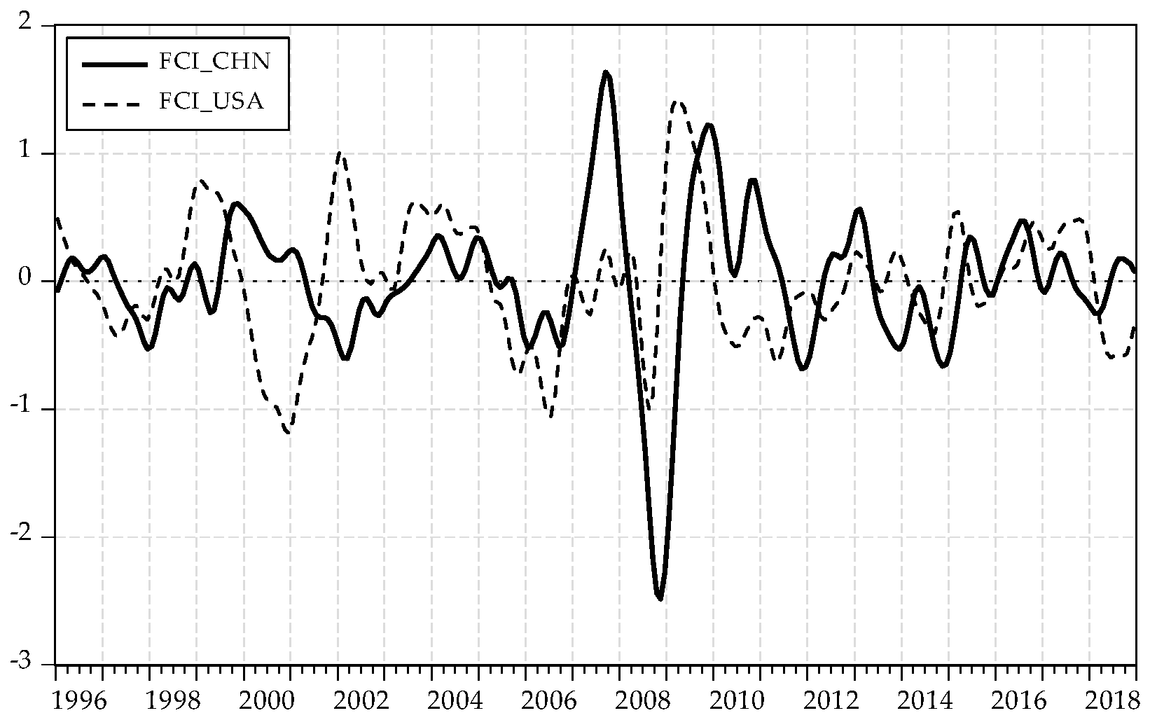
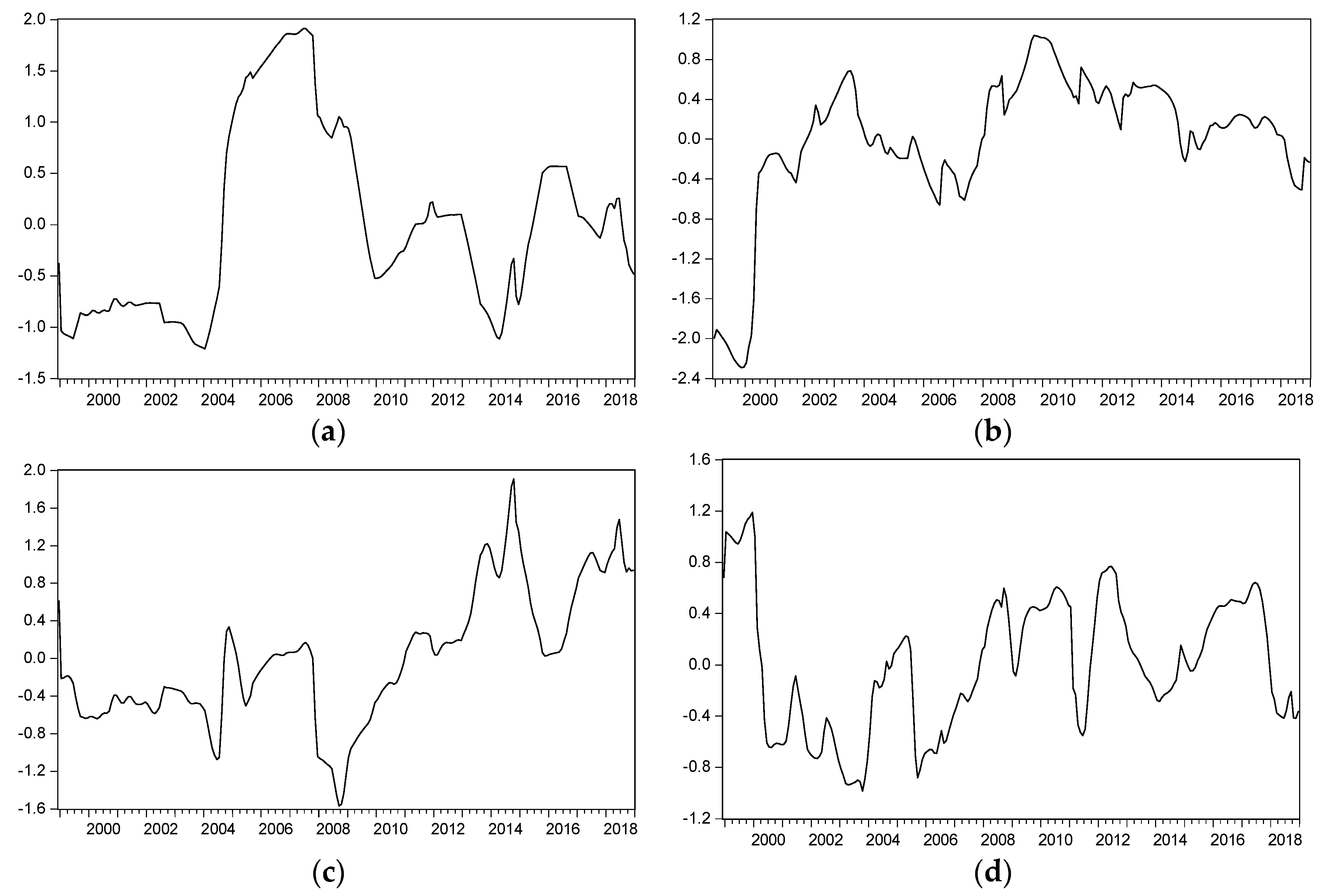
Because the financial indicators used in the calculation of the FCI are all processed by de-trend and standardization, the calculated FCI directly reflects the deviation of a country’s financial activities from the equilibrium state. Specifically, if the value of the FCI is close to zero, it means that the financial environment is in a moderate state; if the FCI is positive (negative), it means that the financial situation is prosperous (recession); if the FCI is rising (falling), it means that the financial situation is getting better (worse).

The key problem is how to determine the weight, $w_i$. A mature method is to use the impulse response function of the VAR model [34]. The weights are determined by measuring the cumulative impact of financial variables on economic growth or inflation. By contrast, the SVAR model not only retains the hypothesis of endogenous variables, but also takes into account the current relationship between variables, so it is more reasonable to determine the weight of variables [36,37]. This paper chooses to use the inflation rate ${\pi }_t$ to form a seven-element SVAR model with six financial variables. The reason for this is mainly based on the following two points: first, China’s GDP data, which characterizes economic growth, can only collect quarterly data, and all data in this paper are monthly data. Second, existing research [35,37] shows that the FCI is generally the leading indicator of economic growth and is more consistent with inflation.

Thus, the following p-order SVAR model is firstly constructed:

$$A{y}_t=A_0^s+A_0^s{y}_{t-1}+\cdots +A_p^s{y}_{t-p}+B{u}_t,$$

(2)

where $y_t=(Ga{p}_{1t},Ga{p}_{2t},\cdots ,Ga{p}_{6t},{\pi }_t{)}^{\prime }$; $A_{7\times 7}$, ${(A_i^s)}_{7\times 7}$, and $B_{7\times 7}$ are structural coefficient matrices; and $u_t$ is the orthonormal unobserved structural innovations with $E(u_t{u^{\prime }}_t)=I_7$. Since A is generally invertible, the corresponding reduced-form VAR model can be obtained:

$$y_t=A^{-1}{A}_0^s+A^{-1}{A}_1^s{y}_{t-1}+\cdots +A^{-1}{A}_p^s{y}_{t-p}+A^{-1}B{u}_t=A_0+A_1{y}_{t-1}+\cdots +A_p{y}_{t-p}+{\epsilon }_t,$$

(3)

and the reduced form error structure is given by

$$\begin{array}{l}A{\epsilon }_t=B{u}_{t}or{\epsilon }_t=A^{-1}B{u}_t=S{u}_t,\\ E({\epsilon }_t{\epsilon }_t^{\prime })=A^{-1}B(A^{-1}B{)}^{\prime }=A^{-1}B{B}^{\prime }{A}^{-1}{}^{\prime }=S{S}^{\prime }.\end{array}$$

(4)

In order to obtain the uniquely determined estimates of the corresponding structural parameters from the simplified parameter estimation, the problem of identification is often encountered [45]. If the constraints are imposed on matrix A and matrix B, they are called AB-model, and the constraints on matrix S are called S-model. The identifying restrictions embodied in the relations $A{\epsilon }_t=B{u}_t$ and ${\epsilon }_t=S{u}_t$ are commonly referred to as short-run restrictions.

Constraints usually come from economic theory, while mature and easily deterministic theories are generally long run. Blanchard and Quah [46] proposed an alternative identification method using restrictions on the long-run properties of the accumulated impulse responses. Based on the model (3), these long-run constraints can be expressed as follows:

$${(I-A_1-A_2-\cdots -A_p)}^{-1}{\epsilon }_t=\mathsf{\Psi }{\epsilon }_t=F{u}_t,$$

(5)

where $\mathsf{\Psi }={(I-A_1-A_2-\cdots -A_p)}^{-1}$ is the long-run multiplier, which may be estimated using the reduced form VAR parameter estimate. It is also evident that $F=\mathsf{\Psi }S$. The SVAR model that imposes constraints on matrix F is called F model. Note that knowledge of $A$ and $B$ is sufficient to compute $S$ or $F$, but the converse is not true. The long-run identifying restrictions are specified in terms of the elements of this matrix $F$, typically in the form of zero restrictions. The restriction $f_{ij}=0$ means that the accumulated response of the i-th variable to the j-th structural shock is zero in the long run.

Considering the economic significance of constraints, this paper chose F model to estimate the weight $w_i$ of the FCI, i.e., long-run constraints are imposed on the SVAR model to satisfy the identifying conditions. According to the principle of SVAR modeling, if there are k variables, at least k(k − 1)/2 constraints must be applied to the matrix F to be identified. Here, we have seven variables, so 21 constraints are required. A common setting method is to set F to the lower triangular matrix. However, if the order of the variables is different, the economic meaning of the constraints will be different. Hence, the ordering of variables is important.

The standardized financial gap variables used in this paper are all converted using the consumer price index (CPI) and can be regarded as real variables. According to the principle of currency neutrality, inflation has no long-term impact on them. At the same time, the calculation of the FCI weight is due to the cumulative reaction of inflation to the impact of various financial variables, so it is assumed that each financial variable has a long-term impact on inflation. Thus, the inflation rate ${\pi }_t$ is ranked as the seventh variable. In addition, it is generally believed that policy variables have long-term effects on other financial variables, while other financial variables do not easily affect policy variables in the long run. Therefore, this paper ranks the broad money supply gap variable and the real interest rate gap variable in the first and second positions. For other variables, the policy tendencies of the variables are ranked in descending order, followed by the social credit loan gap, exchange rate gap, stock price index gap, and house price gap. In fact, the order of the six financial variables is the same as the order shown in Table 1. In the actual estimation, it will also be adjusted based on the estimation results of the F matrix elements. If the element f_ij is not significant, it is adjusted to zero and f_ji set to non-zero. The final form of F is set as follows:

$$F_{CHN}=\begin{array}{cc}& \begin{array}{ccccccc}MS& IR& CL& ER& SP& HP& \pi \end{array}\\ \begin{array}{c}MS\\ IR\\ CL\\ ER\\ SP\\ HP\\ \pi \end{array}& \left[\begin{array}{ccccccc}{f}_{11}& 0& 0& f_{14}& 0& 0& 0\\ f_{21}& f_{22}& 0& 0& 0& 0& 0\\ f_{31}& f_{32}& f_{33}& 0& 0& 0& 0\\ 0& f_{42}& f_{43}& f_{44}& 0& 0& 0\\ f_{51}& f_{52}& f_{53}& f_{54}& f_{55}& f_{56}& 0\\ f_{61}& f_{62}& f_{63}& f_{64}& 0& f_{66}& 0\\ f_{71}& f_{72}& f_{73}& f_{74}& f_{75}& f_{76}& f_{77}\end{array}\right]\end{array}, F_{USA}=\begin{array}{cc}& \begin{array}{ccccccc}MS& IR& CL& ER& SP& HP& \pi \end{array}\\ \begin{array}{c}MS\\ IR\\ CL\\ ER\\ SP\\ HP\\ \pi \end{array}& \left[\begin{array}{ccccccc}{f}_{11}& 0& 0& 0& 0& 0& 0\\ f_{21}& f_{22}& 0& 0& 0& 0& 0\\ f_{31}& f_{32}& f_{33}& 0& 0& 0& 0\\ f_{41}& f_{42}& f_{43}& f_{44}& 0& 0& 0\\ f_{51}& f_{52}& f_{53}& f_{54}& f_{55}& f_{56}& 0\\ f_{61}& f_{62}& f_{63}& f_{64}& 0& f_{66}& 0\\ f_{71}& f_{72}& f_{73}& f_{74}& f_{75}& f_{76}& f_{77}\end{array}\right]\end{array}.$$

(6)

The long-term constraints imposed by China and the United States are basically the same. The main difference is reflected in the long-term effects between the money supply and the exchange rate, i.e., the setting of $f_{41}$ and $f_{14}$. The reason for this setting is that China’s $f_{41}$ is not significant and $f_{14}$ is significant, while the converse is true for the United States. Given the dominant position of the US dollar in the international money market, this result is reasonable.

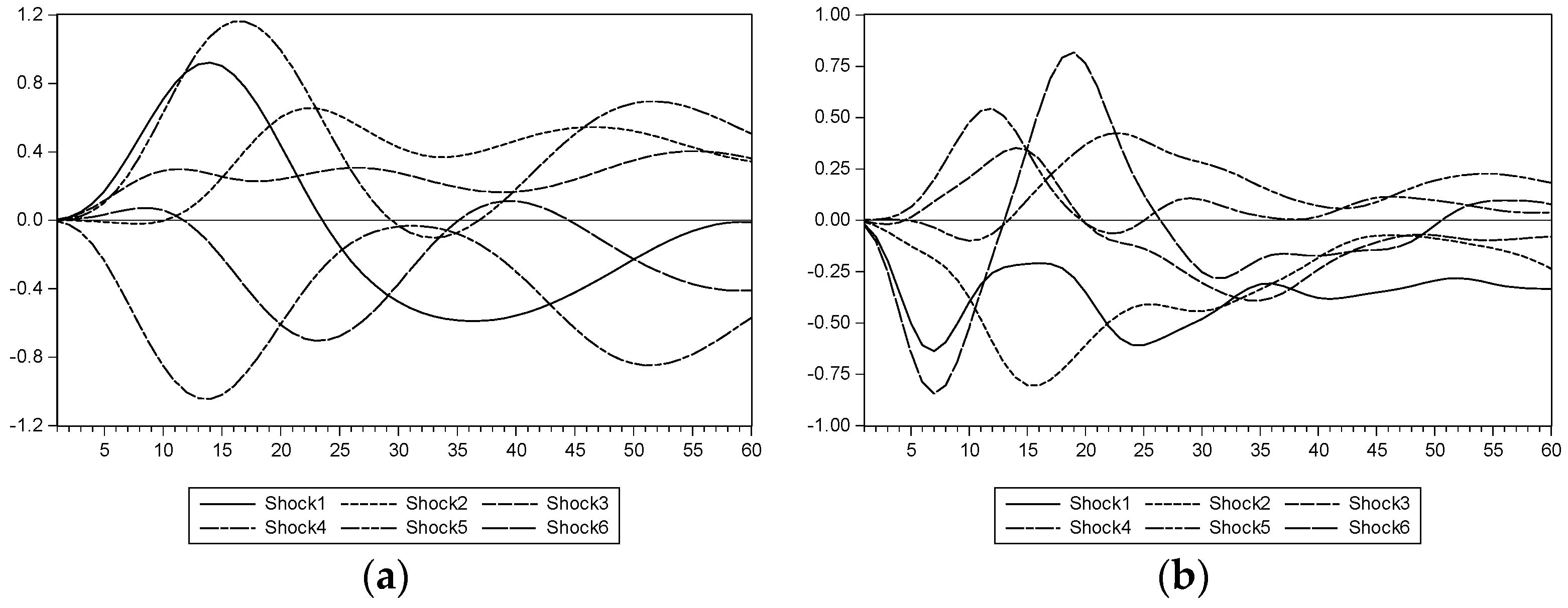
Based on the estimation results of the above SVAR model, the impulse response function is used to further calculate the cumulative response of the inflation rate to the impact of each financial variable. Considering that the short economic cycle is generally 3–5 years [16], this paper selects the cumulative generalized impulse response value of 60 months. Finally, the weight of the i-th financial indicator in the FCI is calculated according to the following formula:

$$w_i=\left|z_i\right|/{\displaystyle {\sum }_{i=1}^6\left|z_i\right|},$$

(7)

where $z_i$ is the 60-stage cumulative generalized impulse response of inflation to the gap value of financial variable, i. Thus, in conjunction with Equation (1), the calculation of the FCI can be completed.

3.3.2. Measurement Method of the Comovement

Before the analysis of the synergy between the financial cycles of China and the United States, it is necessary to first divide the fluctuations of the two financial cycles. In the study of the traditional economic cycle, a turning point method, such as the Bry–Boschan method [47], is widely used to identify the peaks and troughs in the time series cycle. However, the turning point obtained by this method needs to satisfy certain rules. The durations of the cycle and its expansion and contraction phases must all exceed the minimum values set in advance. 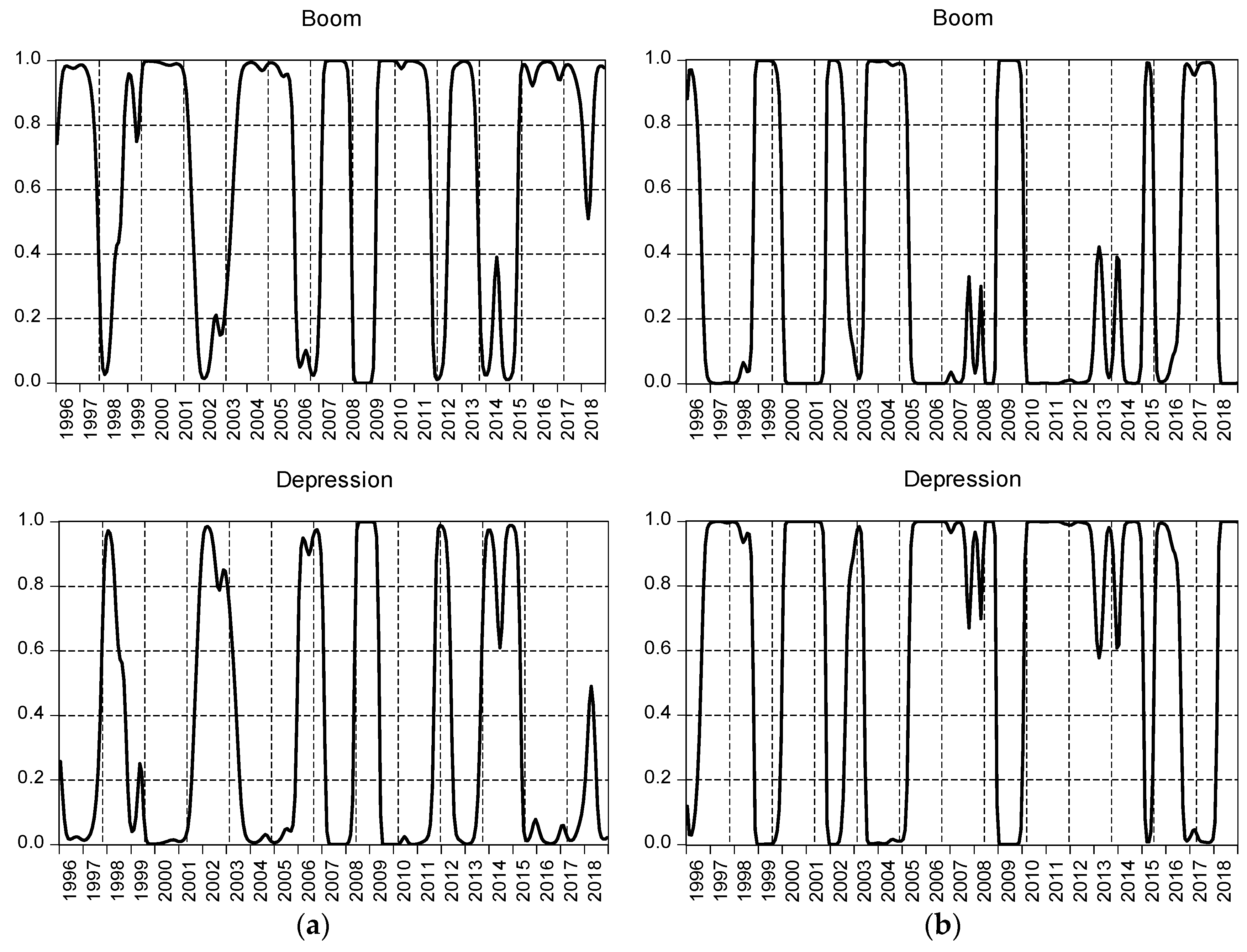In order to avoid artificially set interference, this paper chose the Markov regime switching (MRS) model proposed by Hamilton [48]—in which the turning point is endogenously determined—to identify the fluctuation characteristics of the financial cycle.

Suppose there are two possible states of boom and depression represented by the regime variable, where $s_t$. $s_t=1$ means boom, and $s_t=2$ means depression. In the MRS model, the probability that the t-th period is in a certain regime j depends on the state i during the previous period. Although these probabilities can be set to be time-varying, Markov switching models are generally specified with constant probabilities [49]. The transition probability $p_{ij}$ from regime i in period t − 1 to regime j in period t can be expressed as

$$P(s_t=j|s_{t-1}=i)=p_{ij},$$

(8)

where $p_{ij}\in (0,1)$, $i,j=1$ or 2. We can list these probabilities in a transition matrix as follows:

$$P=\left[\begin{array}{cc}{p}_{11}& p_{12}\\ p_{21}& p_{22}\end{array}\right].$$

(9)

It is easy to see that there should be $p_{11}+p_{12}=1$ and $p_{21}+p_{22}=1$. Typically, we parameterize these probabilities in terms of a logit,

$$p_{11}({\delta }_{11})=\exp ({\delta }_{11})/[\exp ({\delta }_{11})+1]\mathrm{and}{p}_{21}({\delta }_{21})=\exp ({\delta }_{21})/[\exp ({\delta }_{21})+1],$$

(10)

where ${\delta }_{ij}$ are parameters that determine the regime probabilities with the identifying normalizations ${\delta }_{12}=0$ and ${\delta }_{22}=0$. Then, the following MRS model with mean values $\mu (s_t)$ varying with different regimes is constructed:

$$FC{I}_t=\mu (s_t)+{\epsilon }_t,$$

(11)

where ${\epsilon }_t~N(0,\sigma )$. The model (11) is estimated by using the switching regression algorithm in Eviews 10.0 software, and the filtered estimates of the regime probabilities $P(s_t=1|{\Im }_t)$ and $P(s_t=2|{\Im }_t)$ can also be calculated. Here, ${\Im }_t$ is the information set in period, t.

Next, the following indicators are defined for China and the United States, respectively:

$${\rho }_t=\{\begin{array}{c}\begin{array}{cc}1,& ifP(s_t=1|{\Im }_t)>0.5\end{array}\\ \begin{array}{cc}0,& ifP(s_t=1|{\Im }_t)\le 0.5\end{array}\end{array}.$$

(12)

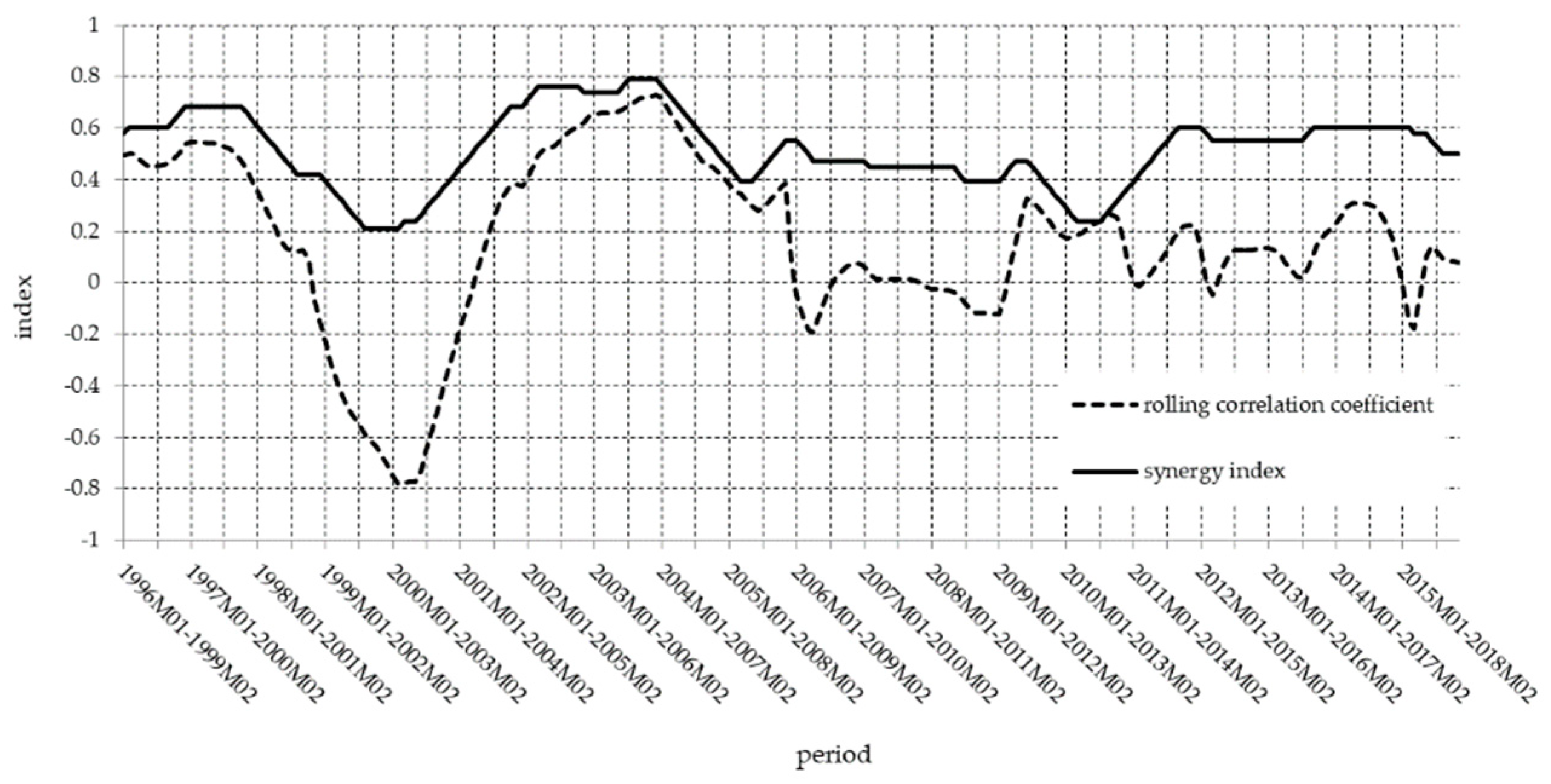
Finally, referring to Harding and Pagan’s method [50,51], a synergy index (SI) is constructed to examine the comovement between the financial cycles of the two countries. The difference is that this paper calculates the rolling form of the T period, where the value of T refers to the summation result of the average duration of each regime estimated by the MRS model, i.e., the average duration of the entire cycle. The specific calculation method of the consistency index is as follows:

$$S{I}_t={\displaystyle {\sum }_{k=t-T+1}^{k=t}[{\rho }_k^{chn}\times }{\rho }_k^{usa}+(1-{\rho }_k^{chn})\times (1-{\rho }_k^{usa})]/T.$$

(13)

It can be seen that the index $S{I}_t$ calculates the proportion of time in which the financial cycles of the two countries are in the same stage (prosperous or depressed) in a complete cycle. Therefore, this paper uses SI to measure the synergy between the financial cycles of China and the United States. Obviously, SI is greater than 0 and less than 1. The closer SI is to 1, the stronger the synchronization of the two cycles.

3.3.3. Analytical Method of Transmission Paths

In theory, financial fundamentals, bilateral trade, and spillover effects of macroeconomic policies can all cause changes in a country’s financial cycle [20,24,31,37]. In order to identify the impact of these factors on the financial cycle synergy between China and the United States, we select and deal with the various influencing factors as follows.

The financial indicators used in the calculation of the FCI in China and the United States already cover the description of financial fundamentals and monetary policy. However, the factor of bank credit loan (CL) was not considered when analyzing risk transmission. First, this is the result of the variable selection based on empirical results when modeling. We did not remove it at the beginning, but its load in each factor is not large in the factor analysis, and its coefficient is also not significant in regression analysis with other factors. Second, we consider that the fluctuation of bank credit loan is an influencing factor of internal financial fluctuations, but it is not a channel for risk transmission between the two countries. For example, the US financial crisis may be related to its own credit expansion, which is one of the reasons for the fluctuation of the US financial market, but the transmission of US financial risks to other countries depends on other paths, such as trade, stock and other asset markets, exchange rates, etc. Considering the limited impact of the domestic credit loan scale on the international market, it should be excluded. Therefore, we calculate the fixed T-period rolling correlation coefficient between the remaining five financial indicators to measure the synergy between the real estate market, stock market, and foreign exchange market, as well as the coordination of monetary policy in the two countries. Noting that the variables for calculating the correlation coefficient need to satisfy the law of large numbers, the stability test will be first performed on each gap sequence in the empirical part. In addition, the T-period moving average growth rate of bilateral trade between China and the United States (expressed by TR) is selected as a proxy indicator for describing trade links. Correspondingly, in this part of the analysis, the dependent variable also selects the T-phase smooth correlation coefficient of the FCIs of the two countries.

Using $Y_{it}^{chn}$ and $Y_{it}^{usa}$ to represent the relevant sequences of China and the United States used in this paper, respectively, the calculation formula of the T-phase rolling correlation coefficient $r_{it}$ of both countries is as follows:

$$r_{it}={\displaystyle {\sum }_{k=t-T+1}^{k=t}[(Y_{ik}^{chn}-{\overline{Y}}_{it}^{chn})}(Y_{ik}^{usa}-{\overline{Y}}_{it}^{usa})]/\sqrt{{\displaystyle {\sum }_{k=t-T+1}^{k=t}{(Y_{ik}^{chn}-{\overline{Y}}_{it}^{chn})}^2}\cdot {\displaystyle {\sum }_{k=t-T+1}^{k=t}{(Y_{ik}^{usa}-{\overline{Y}}_{it}^{usa})}^2}},$$

(14)

where ${\overline{Y}}_{it}^{chn}={\displaystyle {\sum }_{k=t-T+1}^t{Y}_{ik}^{chn}}/T$, ${\overline{Y}}_{it}^{usa}={\displaystyle {\sum }_{k=t-T+1}^t{Y}_{ik}^{usa}}/T$ and $i=(MS,IR,ER,SP,HP,FCI{)}^{\prime }$.

Considering the strong collinearity between independent variables $r_{it}$, $i=(MS,IR,ER,SP,HP,TR{)}^{\prime }$, this paper will extract several common factors with obvious economic significance based on factor analysis. Suppose there are m common factors, denoted by $f_i,i=1,2,\dots ,m$, then the factor model of a single variable can be expressed as

$$r_{it}=l_{i1}{f}_{1t}+l_{i2}{f}_{2t}+\cdots +l_{im}{f}_{mt}+{\upsilon }_{it},$$

(15)

where ${\upsilon }_i$ represents a special factor, which contains a random error, and is only related to the i-th variable, $l_{ij}$ is called the load of the i-th variable on the j-th factor, and the matrix L, which is composed of it, is called the factor load matrix. This can be expressed in matrix form as follows:

$$R_t=L{F}_t+{\upsilon }_t,$$

(16)

where $R_t=(r_{MSt},r_{IRt},r_{ERt},r_{SPt},r_{HPt},r_{TRt}{)}^{\prime }$, $F_t=(f_{1t},f_{2t},\cdots ,f_{mt}{)}^{\prime }$ and ${\upsilon }_t=({\upsilon }_{MSt},{\upsilon }_{IRt},{\upsilon }_{ERt},{\upsilon }_{SPt},{\upsilon }_{HPt},{\upsilon }_{TRt}{)}^{\prime }$.

In order to make the practical meaning of the factor clearer, it is often necessary to orthogonally rotate the load matrix L. Suppose there is an m-dimensional orthogonal matrix H, so that

$$L^{\ast }=LH.$$

(17)

In this paper, the maximum variance rotation method is used to obtain $L^{\ast }$, and then the regression method is used to obtain the estimations of common factors.

$${\widehat{F}}_t={L^{*}}^{\prime }{\mathsf{\Psi }}^{-1}{R}_t,$$

(18)

where $\mathsf{\Psi }$ is the sample correlation matrix.

At the same time, there may be differences in the financial risk transmission paths and transmission effects between China and the United States under different financial cycle synergy levels. Hence, a threshold regression model [52] will be established to test and analyze the transmission paths of financial cooperation between China and the United States. Taking two thresholds as an example, the two thresholds are represented by $V_1$ and $V_2$, and $V_1<V_2$. Then, the model can be constructed as follows

$$r_{FCIt}={\beta }_1{\widehat{F}}_{t}I(S{I}_t\le V_1)+{\beta }_2{\widehat{F}}_{t}I(V_1<S{I}_t\le V_2)+{\beta }_3{\widehat{F}}_{t}I(S{I}_t>V_2)+u_t,$$

(19)

where $I(\cdot )$ is an indicative function. When an event in parentheses occurs, its value is 1.

4. Results

4.1. The Calculation Results of the FCI

The SVAR model requires its endogenous variables to be stationary, so a unit root test is required. This paper chose to use the augmented Dickey–Fuller (ADF) test.

Table 2. Unit root test results (augmented Dickey–Fuller (ADF), at level, without constant and trend).

Null Hypothesis: The Variable Has a Unit Root
CHN	Gap1	Gap2	Gap3	Gap4	Gap5	Gap6	Gap7
t-Statistic	−5.059	−6.3863	−5.4367	−5.7069	−5.6728	−5.8105	−5.1236
Prob.	0.000	0.000	0.000	0.000	0.000	0.000	0.000
	***	***	***	***	***	***	***
USA	Gap1	Gap2	Gap3	Gap4	Gap5	Gap6	Gap7
t-Statistic	−6.0888	−4.1086	−4.437	−5.4806	−5.9417	−5.0096	−8.708
Prob.	0.000	0.000	0.000	0.000	0.000	0.000	0.000
	***	***	***	***	***	***	***

Notes: (*) Significant at the 10% level, (**) significant at the 5% level, (***) significant at the 1% level, and (no) not significant; lag length based on the Schwarz information criterion (SIC); probability based on MacKinnon (1996) one-sided p-values.

illustrates the results, which show that all gap sequences are stable at a 1% significance level.

The maximum lag order of the SVAR model is determined based on five criteria: likelihood ratio (LR), final prediction error (FPE), Akaike information criterion (AIC), Schwarz information criterion (SIC), and Hannan–Quinn information criterion (HQ). The result of determining the lag order is shown in

Table 3. The lag order selections of the structural vector autoregressive (SVAR) model.

	Lag	LR	FPE	AIC	SIC	HQ
CHN	1	NA	4.64 × 10−11	−3.929127	−3.27608	−3.666891
	2	3707.907	3.42 × 10−17	−18.05018	−16.74408	−17.52571
	3	2299.024	4.81 × 10−21	−26.92024	−24.9611	−26.13354
	4	1227.039	4.36 × 10−23	−31.62769	−29.01550 *	−30.57875
	5	174.9147	2.99 × 10−23 *	−32.00904 *	−28.74381	−30.69787 *
	6	68.05228 *	3.21 × 10−23	−31.94456	−28.02627	−30.37114
USA	1	NA	3.14 × 10−11	−4.318835	−3.665788	−4.0566
	2	3091.233	2.58 × 10−16	−16.031	−14.72491	−15.50653
	3	2001.172	1.2 × 10−19	−23.70487	−21.74573	−22.91817
	4	1165.584	1.4 × 10−21	−28.15837	−25.54618	−27.10943
	5	296.2981	5.73 × 10−22 *	−29.05625 *	−25.79102 *	−27.74508 *
	6	66.36510 *	6.2 × 10−22	−28.98436	−25.06608	−27.41095

Note: (*) indicates lag order selected by the criterion (each test at 5% level).

. For both countries, the optimal lag order for more than half of the criteria is 5, so the order of the SVAR model is determined to be 5. Referring to the graphs of the inverse roots of the AR characteristic polynomial, both SVAR models are stable. For the sake of simplicity of the article, no specific figures are given.

For the two identifiable long-term constraint matrices of Equation (6), the estimation results of their parameters are shown in

Table 4. Estimation results of constraint matrix F in SVAR models.

Estimated F_CHN Matrix:
−1.311	0.000	0.000	1.140	0.000	0.000	0.000
−0.862	2.194	0.000	0.000	0.000	0.000	0.000
−3.331	0.412	0.528	0.000	0.000	0.000	0.000
0.000	0.566	1.713	0.215 *	0.000	0.000	0.000
0.835	−0.320	−0.603	−0.571	1.038	−0.021 *	0.000
−0.690	−0.384	−0.781	0.483	0.000	0.935	0.000
−0.255	0.438	0.281	−0.486	0.411	−0.229	0.670
Estimated F_USA Matrix:
1.483	0.000	0.000	0.000	0.000	0.000	0.000
0.657	2.056	0.000	0.000	0.000	0.000	0.000
0.956	−0.830	1.597	0.000	0.000	0.000	0.000
−0.417	−0.467	0.875	1.676	0.000	0.000	0.000
−0.764	−0.713	0.293	0.277	1.003	0.705	0.000
1.289	0.496	0.149	−0.749	0.000	0.976	0.000
−0.360	−0.280	−0.130	0.050 *	0.181	−0.017 *	0.570

Notes: The i-th row and j-th column values in the table represent the estimated values of the i-th row and j-th column elements of the matrix. (*) indicates that the coefficient is not significant at the 5% level.

. Based on this, the structural decomposition method in pulse analysis is further selected to calculate the cumulative impact of unit shock of each financial gap sequence on inflation for 60 months. The results are shown in Figure 1. Next, the weight results calculated according to Equation (7) are shown in

Table 5. Weights of financial indicators calculated based on SVAR model.

	MS	IR	CL	ER	SP	HP
Weights	$w_1$	$w_2$	$w_3$	$w_4$	$w_5$	$w_6$
CHN	0.0048	0.1561	0.1641	0.2588	0.2296	0.1865
USA	0.3527	0.2491	0.0843	0.0391	0.1932	0.0816

. Finally, Figure 2 shows the FCI index calculation results for the two countries.

It can be seen from Figure 2 that from 1996 to 1997, the financial situation in China continued to deteriorate due to insufficient domestic effective demand and Asian financial turmoil. To stimulate demand and ease deflationary pressures, China implemented a series of expansionary financial regulatory policies and reform measures. The FCI began to pick up gradually in 1998. However, with the gradual decline of active fiscal and monetary policies, FCI began to fall back to the vicinity of the zero line since 2000. From the second half of 2001 until the split-share structure reform in 2003, China’s stock market continued to be sluggish, corporate financing was difficult, the FCI value was always less than zero, and the financial situation was tight. Since the second half of 2003, bank credit has increased, and China has experienced a partial overheating of the economy and rising prices, resulting in a loose financial environment. In order to prevent potential risks in the financial system, China adopted a number of macro-control measures aimed at controlling the overheating of investment. With the increase in policy regulation in 2005, China’s financial situation tightened, and this continued until the end of 2006. In 2007, due to the stimulation of the 2008 Olympic Games, China’s economy improved, and the stock market was booming. China’s FCI rose rapidly and reached its peak. At the end of 2007, the US financial crisis affected China, and China’s FCI fell rapidly. It reached its lowest point at the end of 2008, and the rate and the extent of decline were unprecedented. In response to the financial crisis, China implemented timely regulation and launched a package of expansionary policies, known as the “four trillion plan”. In 2009, the FCI rebounded rapidly.

Unfortunately, the European debt crisis followed in 2010. China’s financial situation fell sharply again. In 2012, China’s economic growth fell below 8% for the first time in 14 years. Since then, China entered a new period of medium and low economic growth. Taking this as an opportunity, the Chinese government accelerated and intensified financial reform. One of the main measures taken was that Wenzhou, Shenzhen, and other places have been set up as financial comprehensive reform pilot zones. This “bottom-up” reform mode further straightens the financial jurisdiction of the central and local governments, effectively alleviating the financing difficulties of small and medium-sized enterprises, and improves the economic capacity of financial service entities. In addition, the accelerated speed of the marketization of interest rates and exchange rates has further strengthened the fundamental role of the market in the allocation of financial resources. Therefore, China’s FCI temporarily improved in 2012. However, due to the global economic downturn and internal economic structural problems, the FCI began to decline again in 2013 and went into depression in the latter half of the year until the first half of 2015. With the gradual recovery of the economy, China’s macroeconomic regulation and control returned to “stable”, rather than “positive”, and started a new round of financial reform. After 2015, the FCI fell back to a moderately tight range of fluctuations. It can be seen that the Chinese FCI measured in this paper is a good description of the changes in China’s financial environment, and can be a useful basis for analyzing China’s macroeconomic and financial wave dynamics.

Compared with the changes in the FCI and the financial situation in the United States, in the first half of 1996, the US banking industry was in serious crisis and the FCI continued to decline. With the launch of a series of initiatives such as raising credit card issuance standards, credit quality improved and the FCI began to pick up in early 1997. In the same year, the Asian financial crisis broke out and spread rapidly, leading to the chaos of global financial markets, combined with the bursting of the IT bubble in 2000 and the impact of the “911” incident, all of which contributed to a persistent sluggish financial situation in the United States. Its FCI declined from the end of 1998 and remained in a tight state until the second half of 2001. In order to restore the economy, the Federal Reserve cut interest rates 13 times between January 2001 and June 2003, and achieved the lowest interest rate since 1958, making the US financial market unprecedentedly active and causing large amounts of funds to flow into the real estate market. However, there was no interest rate cutback for quite a long time afterwards, which created a hidden danger for the financial crisis.

In 2007, the sub-loan crisis broke out in the United States, from the credit crisis to the Wall Street financial crisis, and then triggered severe shocks in major stock markets around the world. The FCI in the United States continued to decline. In response, the United States successively passed the “A package of economic stimulus bills” with a total tax reduction of 168 billion dollars, launched the “Emergency Economic Stability Act of 2008” with a 700 billion non-performing asset rescue plan, and implemented the “Recovery and Reinvestment Act of the United States” with an increase of 787 billion dollars in fiscal expenditure. Through a series of economic stimulus plans, the financial situation began to return to moderately loose range fluctuations in 2010. Subsequently, the United States was also affected by the European debt crisis and the deterioration of the global economic situation, and the financial state also experienced a long downturn. With the recovery of the US economy, the financial situation returned to a moderate overall good trend in 2013. Therefore, it can be seen that the changes in the US FCI are also consistent with the volatility reality of the overall financial situation. Reasonable FCI calculations in China and the United States ensure the reliability of subsequent analysis.

4.2. Comovement of China–US Financial Cycle

This section first uses the MS model to identify the financial cycles of China and the United States based on the FCI calculated previously, and then calculates the consistency index according to Equations (12) and (13).

Table 6. Money supply (MS) model estimation results of financial cycles in China and the United States.

	Parameters	CHN	USA
Boom	μ(st = 1)	0.2388 ***	0.5177 ***
Depression	μ(st = 2)	−0.4988 ***	−0.2634 ***
Regime maintenance probability	p11	0.9648	0.9246
	p22	0.9210	0.9602
Expected duration of boom		28.3869	13.2700
Expected duration of depression		12.6594	25.1413

Note: (***) Significant at the 1% level.

shows the results of the stage division of financial cycle fluctuations. From the results of the estimated mean of the two regimes, it can be seen that the two states of boom and depression are well-identified by the model. Moreover, for both countries, the maintenance probability of both states is high, showing a more stable feature. Further comparing the durations of the different stages of the two financial cycles, we can find that the financial cycle fluctuations of China and the United States both have significant asymmetry characteristics. The average length of prosperity and depression in China’s financial cycle is 28.4 and 12.7 months respectively, which is characterized by the asymmetry of “long prosperity and short depression”; while the average length of the corresponding two states in the United States is 13.3 and 25.1 months, which is characterized by the asymmetry of “long depression and short prosperity”. In addition, China’s financial cycle is about 41 months, and is about 38 months for the United States. These results are basically consistent with the conclusions of the existing literatures [32,36,38,39,40].

Further calculating the filtered regime probabilities of the FCI (see Figure 3 for the results) identifies two states of the financial cycle. The result of the synergy index calculated by Equation (13) is finally obtained. Since a complete financial cycle in the United States is 38 months (less than 41 months in China), the results of the 38-phase rolling synergy index are calculated by Equation (13). The results are given in Figure 4, which also shows the 38-phase rolling correlation coefficient of the two FCIs calculated according to Equation (14) as a reference.

Figure 4 shows that the synergy of the financial cycles between China and the United States has obvious time-varying characteristics. Since the mid-1990s, China and the United States have continued to develop their economies, and their trade relations and financial and economic exchanges have entered a period of rapid development. The synergy of the financial cycle has risen remarkably. Especially during the period of Asian financial turmoil, the financial cycles of the two countries experienced a high degree of synergy. As China–US economic relations became increasingly close, the imbalance in economic relations between the two countries gradually intensified. Not only did the imbalance between the huge trade deficit of the United States and the huge surplus of China occur, but it also showed an imbalance between the investment of the United States in China, mainly in stock investment, and that of China in the United States, mainly in bond investment. The financial cycle comovement between the two countries fluctuated at a low level between 2000 and 2002, and even decoupling occurred. As China joins the World Trade Organization and integrates into the global economy, the dependence between China and the United States on commodity markets and financial markets has also deepened. During the US financial crisis in 2009, the synergy between the financial cycles of the two countries rose sharply and reached a maximum due to the homogeneity of policies. After the crisis broke out, China’s exports to the United States fell sharply. The financial crisis intensified the prominence of the severity of the Dollar Trap, which prompted the Chinese government to diversify its foreign exchange reserves to gradually eliminate its dependence on the US financial market. Therefore, the synchronicity of the financial cycles of the two countries in 2009–2011 was basically in an irrelevant state. After 2012, as the US economy recovered and the Chinese economy entered a period of moderate growth adjustment, and the synergy between the financial cycles of the two countries was basically maintained at a stable period of around 0.6.

In summary, the synergy of the financial volatility between China and the United States has changed significantly in recent years. Especially during the two financial crises, the financial cycle synergy of the two countries was significantly higher than other periods. On the one hand, this illustrates the existence of financial risk contagion effects among countries. On the other hand, it can also reflect the strengthening of coordination and cooperation among countries in policy control when faced with risks. In addition, the comovement of financial volatility between China and the United States has both high levels of cooperation in response to crises and abandonment of each other in the game of their respective interests. Therefore, this time-varying nonlinear feature should be considered when analyzing the coordination or risk conduction path. In other words, the factors affecting the financial cycle synergy between China and the United States may differ during different periods, and the mechanisms and driving forces for financial risks to spread between the two countries may also undergo important changes.

5. Discussion on Transmission Paths

This section will discuss the conduction paths of the financial cycles of the two countries. Specifically, the potential common factors are first refined, and then a threshold regression model is established to analyze the conduction paths under different levels of synergy.

According to Equation (16), factor analysis is carried out on six indicators that represent the correlation between trade, asset market, and policy in the two countries. According to the criterion that the eigenvalue is greater than 1, the number of selected factors is m = 4, and the estimated result of the load matrix L is shown in

Table 7. Load matrix estimation results in factor analysis.

Unrotated Loadings L	f1	f2	f3	f4
rMS	0.7727	−0.0025	0.2997	−0.0722
rIR	0.0437	−0.3135	0.1454	0.3777
rER	−0.0837	0.2358	0.5316	−0.0859
rSP	0.2974	0.5680	−0.2279	0.0058
rHP	−0.0802	0.4656	0.0743	0.3058
rTR	0.8543	−0.1126	−0.1401	0.0642
Contribution ratio	0.5002	0.2468	0.1646	0.0884
Cumulative contribution ratio	0.5002	0.7470	0.9116	1.0000
Rotated Loadings: L*	f1	f2	f3	f4
rMS	0.7986	0.0000	0.2323	−0.0209
rIR	0.0849	−0.1913	−0.0307	0.4682
rER	−0.0465	0.0355	0.5909	−0.0082
rSP	0.2074	0.6118	−0.0447	−0.2091
rHP	−0.1272	0.4883	0.1828	0.1851
rTR	0.8387	0.0700	−0.2392	0.0243

. Furthermore, the load matrix is orthogonally rotated according to the principle of variance maximization, and the result of the rotated load matrix L* is also shown in Table 7. It can be seen from the results that the cumulative contribution rate of the four common factors for the variance of the original variables is 1, indicating that the six variables are perfectly reduced to four dimensions by factor analysis.

According to the rotational load of each common factor, $r_{MS}$—which represents the trade correlation between the two countries—has the largest load on the common factor $f_1$; hence, $f_1$ is called the trade factor. The correlations between stock prices and between house prices in both countries have higher loads on factor $f_2$, so $f_2$ is defined as an asset factor. According to the same principle, factor $f_3$ and factor $f_4$ are defined as the exchange rate factor and the interest rate factor, respectively.

In addition, $r_{MS}$, which indicates the correlation of the supply of the national currency, has a load of up to 0.7986 factor $f_1$, but the issuance of money in the external economy is more useful for balancing trade balances and stable exchange rates, so the definition of the factor name is not used. Its load on the exchange rate factor $f_3$ also reaches 0.2323, while the load on the other two factors is very small. These results also prove the rationality of such treatment. After obtaining a stable factor rotation result, the factor score sequences can be calculated according to Equation (18) for characterizing the fluctuation of each common factor. This paper selected the regression method to predict these four common factors, and the results are shown in Figure 5.

Finally, the four factors obtained are used as explanatory variables, and the threshold regression analysis of the rolling correlation coefficient $r_{FCIt}$ is performed. The synergy index SI is chosen as the threshold variable. The threshold test results of

Table 8. Multiple threshold tests.

Threshold Test 1	F-Statistic	Scaled F-Statistic	Critical Value 2
0 vs. 1 *	44.095	220.477	22.400
1 vs. 2 *	34.271	171.357	24.420
2 vs. 3	4.689	23.443	25.530
Threshold Values: 0.361, 0.583

Notes: ¹ Method: Bai–Perron tests of L + 1 vs. L sequentially determined, ² Bai–Perron critical values, and (*) significant at the 0.01 level.

show that there are two thresholds at the significance level of 0.01 with values of 0.361 and 0.583.

According to the threshold regression results in

Table 9. Threshold regression results.

Threshold Interval	f1 (Trade)	f2 (Asset)	f3 (Exchange Rate)		f4 (Interest Rate)
SI < 0.361	0.4690 *	−0.1361	0.5251 *		0.0533
0.361 ≤ SI < 0.583	0.1032 *	0.2056 *	0.0073		0.1999 *
0.583 ≤ SI	0.1012 *	0.1816 *	−0.1210 *		−0.1409 *
R-squared	0.8464	Adjusted R-squared		0.8369
F-statistic	88.5767	Prob. (F-statistic)		0.0000

Note: (*) Significant at the 0.05 level.

, we can make an intuitive judgment about the main factors affecting the synergy of financial cycles between China and the United States. When the synergy is at a low level (i.e., less than 0.361), the growth of bilateral trade and the enhanced correlation of exchange rates are the main reasons for the increase in the synergy of financial cycles between China and the United States. With the improvement of the level of synergy, when it is at a medium level (i.e., between 0.361 and 0.583), the linkages of trade growth, stock market, real estate market, and interest rate policy between the two countries become important. When the level of synergy reaches a high level (i.e., greater than 0.583), the linkage of trade, house price, stock price, exchange rate, and interest rate can all cause the change in financial cycle synergy between the two countries. However, two policy-related factors, such as the exchange rate and interest rate, have a negative effect. Thus, under different levels of financial cycle synergy, the main factors that cause the change in financial cycle synergy between China and the United States are obviously different.

The above results confirm that the strengthening of bilateral trade is the basis of the financial cycle linkage because the coefficient of trade factor is significant at each threshold interval. Simultaneously, it also implies that some important changes have taken place in the transmission channels of financial risks, with the change of macroeconomic and financial market linkages between China and the United States.

The financial link between the two countries is generally poor when the level of trade between the two countries is low. In an open economy, a country’s net capital outflow is always equal to net exports. When there is a trade surplus, capital flows out, and when there is a trade deficit, capital flows in. The flow of capital between the two countries is basically dependent on the income and expenditure of the goods trade. As the trade between the two countries continues to strengthen, the importance of the foreign exchange market will first increase significantly, so the exchange rate channel becomes the main mechanism for financial shock and risk transmission between the two economies. Due to the closer relationship between the two countries with respect to economic and financial activities, the linkage of asset prices—which is represented by stock prices and housing prices—has become the main driving factor for the coordinated movement of the financial cycle. The capital market becomes the main channel for the transmission of international financial risks. In addition, the interest rate factor also shows a positive increase. On the one hand, this means that using foreign currency accumulated by trade to purchase foreign bonds with interest has become an important means of financial linkage between the two countries. On the other hand, it also implies that the two countries have not yet felt an urgent need to coordinate the use of macro-control policies to cope with the global financial crisis or economic recession. When the financial cycles of China and the United States showed a high degree of synergy—mainly during the two financial crises—the financial market volatility of the two countries was highly correlated. At this time, trade and asset factors were still the main means by which to link the financial cycle. However, in order to cope with the impact of the financial crisis, the exchange rate factors and interest rate factors which can represent the coordination of monetary policy—such as money supply, exchange rate, and interest rate—have obviously decoupled the financial cycles of the two countries.

6. Conclusions

This paper selects six financial indicators: money supply, interest rate, credit loans, exchange rate, stock price, and house prices in China and the United States. By using the SVAR model and the impulse response function to determine the weights of financial indicators, we synthesized the financial conditions indices (FCIs) of the two countries. Combined with the actual financial situation of the two countries, the two FCIs constructed in this paper can better reflect reality, so they offer a useful basis for analyzing the fluctuation of the financial cycle in the two countries.

The results of the stage division of the financial situation index based on the MS model show that the lengths of the financial period in China and the United States are 41 months and 38 months, respectively. Another finding is that the financial cycle fluctuations of the two countries have distinct asymmetry features. The US financial cycle is characterized by a period of “long depression and short prosperity”, while China’s financial cycle is characterized by long prosperity and a short depression”. Therefore, in the process of formulating and implementing macroeconomic regulation, control policies, and financial reform policies, the Chinese government should control the intensity of the implementation of expansionary policies to prevent excessive responses to the deterioration of the financial situation.

Furthermore, this paper constructs and calculates the synergy index (SI) to measure the synergy of the financial cycle between China and the United States. We found that the synergy of the financial cycles of the two countries has changed significantly in the past two decades. Especially during the two financial crises, the financial cycles in China and the United States showed a high degree of synergy. This implies that we should pay attention to nonlinear problems in the regression analysis of the subsequent impact paths.

In order to avoid the influence of the collinearity between variables on the estimation results in the analysis of the conduction path of the financial cycle, the four common factors of trade, assets, exchange rate, and interest rate are first compacted by using factor analysis. The results of the threshold test show that there are two thresholds, i.e., 0.361 and 0.583, when the synergy index (SI) is used as the threshold variable. Finally, the threshold regression results show that the trade factor is the basis of the financial cycle synergy. When the synergy is at a low level (SI < 0.361), the exchange rate factor is the main cause of the financial cycle comovement change, and also the main channel of international financial risk. As the financial cycle synergy increases (0.361 ≤ SI < 0.583), the asset factor and interest rate factor start to become the main reason for the changes in the financial cycle synergy. When the level of synergy breaks through 0.583, the capital factor based on stock prices and house price is still the main path of financial market linkage and risk transmission, but the linkage of monetary policy between the two countries shows a restraining effect on synergy.

In summary, the policy implications for China include the following points: China should strengthen the relevant monitoring of its own financial cycle and its major trading partners in order to cope with external risks in a timely and correct manner. If the synergy of the financial cycle is low, we should pay greater attention to the transmission of financial risks between foreign exchange markets. When the financial cycle synergy of the two countries reaches a high level and the capital market becomes the main transmission mechanism of financial risk, we should carefully observe the fluctuation of domestic and foreign capital markets and establish a certain isolation mechanism to control the further spread of financial risk. At the same time, we should focus on the coordinated use of macroeconomic regulation and control policies, especially monetary policies, with other countries to jointly resist the transmission impact of financial shocks on the real economy.

For the United States, the above recommendations are still applicable. However, considering the importance of the United States in international financial markets, such as foreign exchange and securities as well as in trade, the United States should give due consideration to the impact on other countries’ financial and economic aspects while implementing its own regulatory policies. In addition, attention should be paid to the fundamental role of trade in financial linkages.

Our study also suffers from some limitations. In this paper, the synchronicity index or the rolling correlation coefficient is used to measure the financial synchronicity between China and the United States, and it is used as an explanatory variable to analyze the transmission of financial risk. This actually implies that the transmission of risk between China and the United States is symmetrical. In reality, it is likely that the impact of China’s financial shock on US finance and the impact of US financial shock on China’s finance are asymmetric. Therefore, asymmetry in the financial relationship between China and the United States may be the direction of future research.

References

1. Jiang, Y.; Li, C.; Zhang, J.; Zhou, X. Financial Stability and Sustainability under the Coordination of Monetary Policy and Macro prudential Policy: New Evidence from China. Sustainability 2019, 11, 1616. [Google Scholar] [CrossRef]
2. Nyblom, A.; Isaksson, K.; Sanctuary, M.; Fransolet, A.; Stigson, P. Governance and Degrowth: Lessons from the 2008 Financial Crisis in Latvia and Iceland. Sustainability 2019, 11, 1734. [Google Scholar] [CrossRef]
3. Ehrmann, M.; Fratzscher, M.; Rigobon, R. Stocks, Bonds, Money Markets and Exchange Rates: Measuring International Financial Transmission. J. Appl. Econ. 2011, 26, 948–974. [Google Scholar] [CrossRef]
4. Caruana, J.; Borio, C.; Shin, H.S. 84th Annual Report: 2013–2014; BIS Annual Report; Bank for International Settlements: Basel, Switzerland, 2014. [Google Scholar]
5. Borio, C. The financial cycle and macroeconomics: What have we learnt? J. Bank. Financ. 2014, 45, 182–198. [Google Scholar] [CrossRef] [Green Version]
6. World Bank Open Data. Available online: https://data.worldbank.org.cn/ (accessed on 27 July 2019).
7. Fisher, I. The Debt-Deflation Theory of Great Depressions. Econometrica 1933, 1, 337–357. [Google Scholar] [CrossRef]
8. Lucas, R.E. Econometric Policy Evaluation: A Critique. In Carnegie-Rochester Conference Series on Public Policy; North-Holland Publishing Company: Amsterdam, The Netherlands, 1976; pp. 19–46. [Google Scholar]
9. Kydland, F.E.; Prescott, E.С. Time to Build and Aggregate Fluctuations. Econometrica 1982, 50, 1345–1370. [Google Scholar] [CrossRef]
10. Nelson, C.R.; Plosser, C.R. Trends and Random Walks in Macroeconomic Time Series: Some Evidence and Implications. J. Monet. Econ. 1982, 10, 139–162. [Google Scholar] [CrossRef]
11. Woodford, M.; Walsh, C.E. Interest and Prices: Foundations of a Theory of Monetary Policy. Macroecon. Dyn. 2005, 9, 462–468. [Google Scholar] [CrossRef]
12. Bernanke, B.S.; Gertler, M.; Gilchrist, S. The Financial Accelerator in a Quantitative Business Cycle Framework. In Handbook of Macroeconomics; Taylor, J.B., Woodford, M., Eds.; Elsevier: Amsterdam, The Netherlands, 1999; Volume 1, pp. 1341–1393. [Google Scholar]
13. Kashyap, A.K.; Stein, J.C. Cyclical Implications of the Basel II Capital Standards. Econ. Perspect. Fed. Reserve Bank Chic. 2004, 28, 18–33. [Google Scholar]
14. Adrian, T.; Shin, H.S. Financial Intermediaries and Monetary Economics. In Handbook of Monetary Economics; Friedman, B.M., Woodford, M., Eds.; Elsevier: Amsterdam, The Netherlands, 2010; Volume 3, pp. 601–650. [Google Scholar]
15. Mimir, Y. Financial Intermediaries, Credit Shocks and Business Cycles. Oxf. Bull. Econ. Stat. 2016, 78, 42–74. [Google Scholar] [CrossRef]
16. Dell Ariccia, G.; Igan, D.; Laeven, L.U. Credit Booms and Lending Standards: Evidence from the Subprime Mortgage Market. J. Money Credit Bank. 2012, 44, 367–384. [Google Scholar] [CrossRef] [Green Version]
17. Claessens, S.; Kose, M.A.; Terrones, M.E. How Do Business and Financial Cycles Interact? J. Int. Econ. 2012, 87, 178–190. [Google Scholar] [CrossRef]
18. Drehmann, M.; Borio, C.; Tsatsaronis, K. Characterizing the Financial Cycle: Don’t Lose Sight of the Medium Term; BIS Working Paper No. 380; Bank for International Settlements: Basel, Switzerland, 2012. [Google Scholar]
19. Jorda, O.; Schularick, M.; Taylor, A. When Credit Bites Back: Leverage, Business Cycles and Crises; NBER Working Paper No. 17621; National Bureau of Economic Research: Cambridge, MA, USA, 2011. [Google Scholar]
20. Schularick, M.; Taylor, A.M. Credit Booms Gone Bust: Monetary Policy, Leverage Cycles, and Financial Crises, 1870–2008. Am. Econ. Rev. 2012, 102, 1029–1061. [Google Scholar] [CrossRef]
21. Aikman, D.; Haldane, A.G.; Nelson, B.D. Curbing the Credit Cycle. Econ. J. 2014, 125, 1072–1109. [Google Scholar] [CrossRef]
22. Goodhart, C.; Hofmann, B. Others, Asset Prices, Financial Conditions, and the Transmission of Monetary Policy. In Conference on Asset Prices, Exchange Rates, and Monetary Policy, Stanford University; Stanford University: Stanford, CA, USA, 2001; pp. 2–3. [Google Scholar]
23. English, W.; Tsatsaronis, K.; Zoli, E. Others Assessing the Predictive Power of Measures of Financial Conditions for Macroeconomic Variables. BIS Pap. 2005, 22, 228–252. [Google Scholar]
24. Hatzius, J.; Hooper, P.; Mishkin, F.S.; Schoenholtz, K.L.; Watson, M.W. Financial Conditions Indexes: A Fresh Look after the Financial Crisis; NBER Working Paper No. 16150; National Bureau of Economic Research: Cambridge, MA, USA, 2010. [Google Scholar]
25. Hakkio, C.S.; Keeton, W.R. Financial Stress: What is It, How Can It be Measured, and Why Does It Matter? Econ. Rev. 2009, 94, 5–50. [Google Scholar]
26. Cardarelli, R.; Elekdag, S.; Lall, S. Financial Stress and Economic Contractions. J. Financ. Stab. 2011, 7, 78–97. [Google Scholar] [CrossRef]
27. Molenaar, P.C.; De Gooijer, J.G.; Schmitz, B. Dynamic Factor Analysis of Nonstationary Multivariate Time Series. Psychometrika 1992, 57, 333–349. [Google Scholar] [CrossRef]
28. Menden, C.; Proano, C.R. Dissecting the Financial Cycle with Dynamic Factor Models. Quant. Financ. 2017, 17, 1965–1994. [Google Scholar] [CrossRef]
29. Brave, S.A.; Butters, R. Monitoring Financial Stability: A Financial Conditions Index Approach. Econ. Perspect. 2011, 35, 22–43. [Google Scholar]
30. Matheson, T.D. Financial Conditions Indexes for the United States and Euro Area. Econ. Lett. 2012, 115, 441–446. [Google Scholar] [CrossRef]
31. Dudley, W.; Hatzius, J. The Goldman Sachs Financial Conditions Index: The Right Tool for a New Monetary Policy Regime; Global Economics Paper No. 44; Goldman Sachs: New York, NY, USA, 2000. [Google Scholar]
32. Montagnoli, A.; Napolitano, O. Financial Condition Index and Interest Rate Settings: A Comparative Analysis. In Money Macro and Finance (MMF) Research Group Conference 2004; Money Macro and Finance Research Group: London, UK, 2004; p. 1. [Google Scholar]
33. Wang, X. Financial Conditions Index and Monetary Policy Intermediary Target. J. Shanxi Financ. Econ. Univ. 2009, 31, 95–101. [Google Scholar]
34. Swiston, A.J. A US Financial Conditions Index: Putting Credit Where Credit is Due; International Monetary Fund Working Papers No. 8; International Monetary Fund: Washington, DC, USA, 2008. [Google Scholar]
35. Feng, S.; Jiang, F.; Xie, Q.; Zhang, W. Mechanism and Empirical Analysis of Inflation Trends Forecasting by Financial Conditions Index: Based on China’s Monthly Data from 1999 to 2011. China Ind. Econ. 2012, 289, 18–30. [Google Scholar]
36. Xu, G.; Zheng, W. Construction and Predictive Ability Research on China’s Financial Conditions Index. Stat. Res. 2013, 30, 17–24. [Google Scholar]
37. Deng, C.; Xu, M. The Interaction between Financial Cycle and Business Cycle in China: An Empirical Analysis Based on the Dynamic Spillover Index. J. Shanghai Univ. Financ. Econ. 2018, 20, 63–76. [Google Scholar]
38. Xiang, W.; Wang, D. On the Asymmetry of Sino-U.S. Financial Interdependence. World Econ. Study 2011, 209, 10–16. [Google Scholar]
39. Yu, Z.; Xu, X. Is the Sino-US financial market linkage after the “subprime mortgage crisis” stronger? Economist 2014, 9, 87–95. [Google Scholar]
40. Drehmann, M.; Tsatsaronis, K. The credit-to-GDP Gap and Countercyclical Capital Buffers: Questions and Answers. BIS Q. Rev. 2014, 19, 55–73. [Google Scholar]
41. Zhu, T.; Huang, H. China’s Financial Cycle: Indicators, Methods and Empirical Research. J. Financ. Res. 2018, 462, 55–71. [Google Scholar]
42. CEInet Statistics Database. Available online: http://db.cei.gov.cn (accessed on 31 May 2019).
43. The Official Website of the Bank for International Settlements. Available online: https://www.bis.org/ (accessed on 31 May 2019).
44. The Federal Reserve Website. Available online: https://www.federalreserve.gov/ (accessed on 31 May 2019).
45. Amisano, G.; Giannini, C. Topics in Structural VAR Econometrics, 2nd ed.; Springer Science and Business Media: Berlin, Germany, 2012. [Google Scholar]
46. Blanchard, O.J.; Quah, D. The Dynamic Effects of Aggregate Demand and Aggregate Supply. Am. Econ. Rev. 1989, 79, 655–673. [Google Scholar]
47. Bry, G.; Boschan, C. Cyclical Analysis of Time Series: Selected Procedures and Computer Programs; NBER Working Paper No. 13; National Bureau of Economic Research: Cambridge, MA, USA, 1971. [Google Scholar]
48. Hamilton, J.D. A New Approach to the Economic Analysis of Nonstationary Time Series and the Business Cycle. Econom. J. Econom. Soc. 1989, 57, 357–384. [Google Scholar] [CrossRef]
49. Hamilton, J.D. Specification Testing in Markov-switching Time-Series Models. J. Econom. 1996, 70, 127–157. [Google Scholar] [CrossRef]
50. Harding, D.; Pagan, A. Dissecting the Cycle: A Methodological Investigation. J. Monet. Econ. 2002, 49, 365–381. [Google Scholar] [CrossRef]
51. Harding, D.; Pagan, A. Synchronization of Cycles. J. Econom. 2006, 132, 59–79. [Google Scholar] [CrossRef]
52. Hansen, B.E. Sample Splitting and Threshold Estimation. Econometrica 2000, 68, 575–603. [Google Scholar] [CrossRef] [Green Version]
Figure 1. (a) Accumulated response of GAP7_CHN to innovations; (b) Accumulated response of GAP7_USA to innovations.
Sustainability 11 04151 g001
Figure 2. Calculation results of financial conditions index (FCI) in China and the United States.
Sustainability 11 04151 g002
Figure 3. Markov switching filtered regime probabilities. (a) FCI of China; (b) FCI of the United States.
Sustainability 11 04151 g003
Figure 4. The synergy index and correlation coefficient of the financial cycles.
Sustainability 11 04151 g004
Figure 5. Score sequences of common factors: (a) trade factor f1; (b) asset factor f2; (c) exchange rate factor f3; (d) interest rate factor f4.
Sustainability 11 04151 g005