Market Power and Technology Diffusion in an Energy-Intensive Sector Covered by an Emissions Trading Scheme

Abstract
1. Introduction
2. Materials and Methods
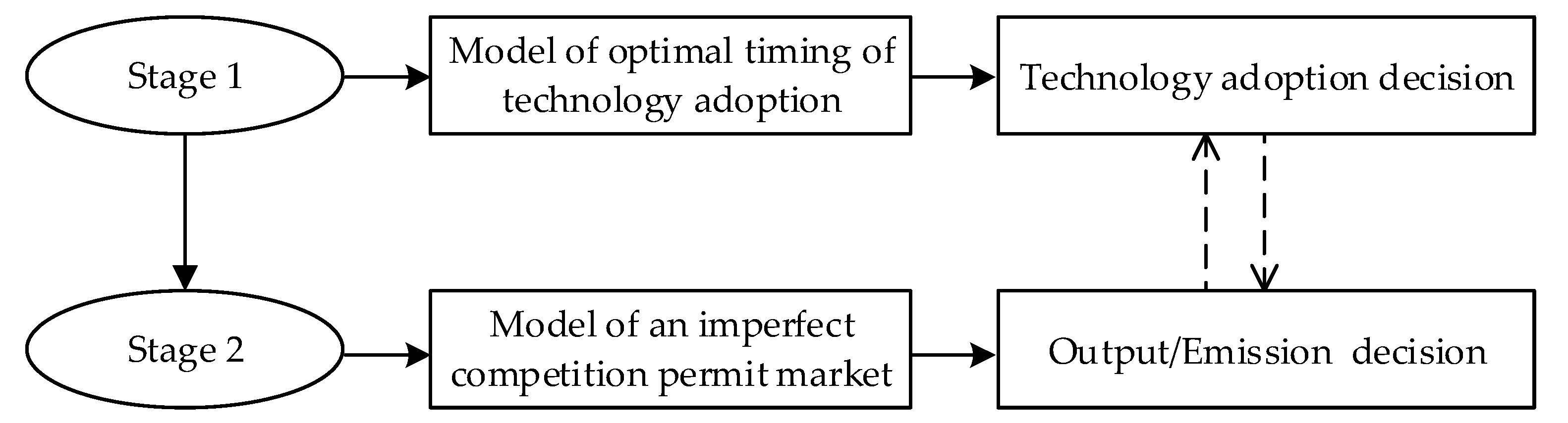
2.1. Model of an Imperfect Competition Permit Market
2.2. Model of Optimal Timing of Technology Adoption
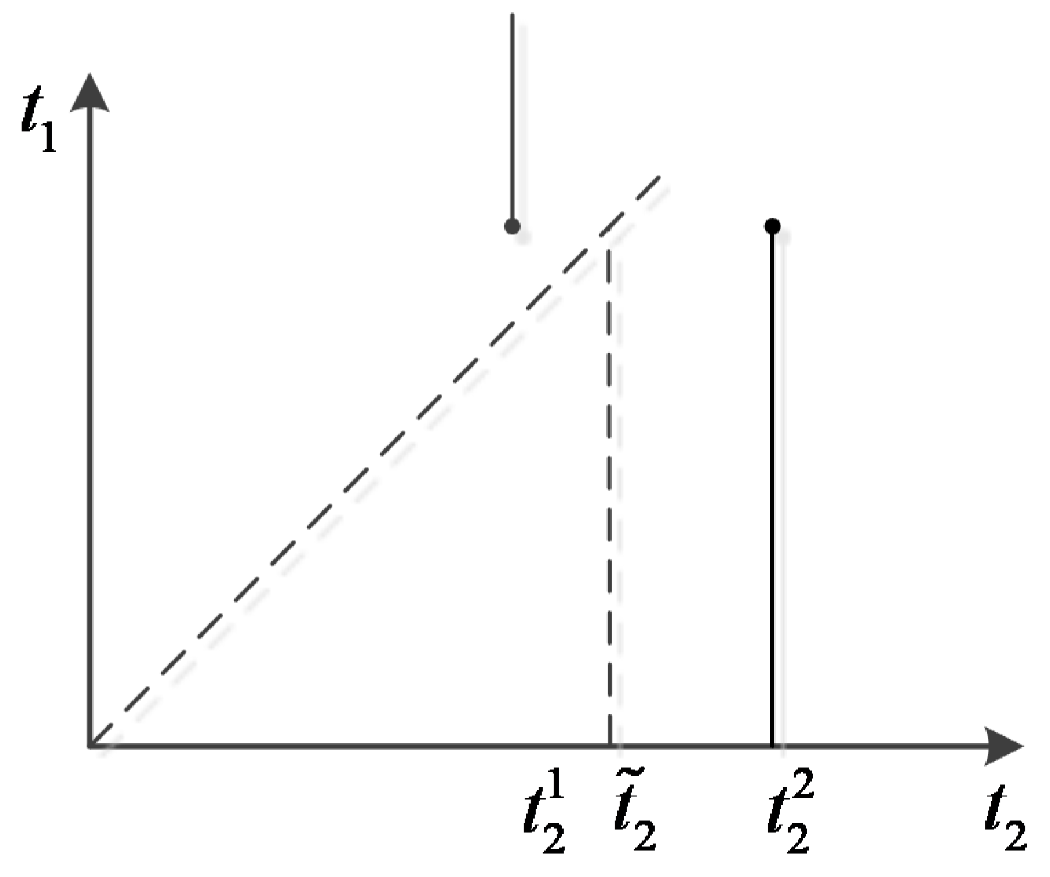
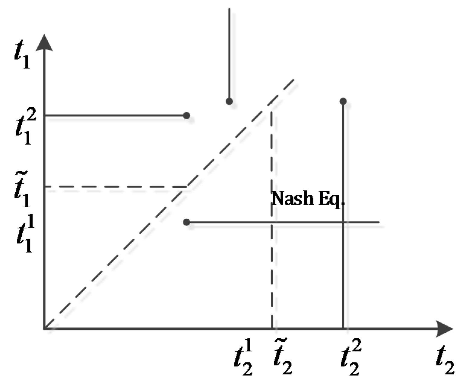
- (1)
- Ifor, then there exists a unique Nash equilibrium.
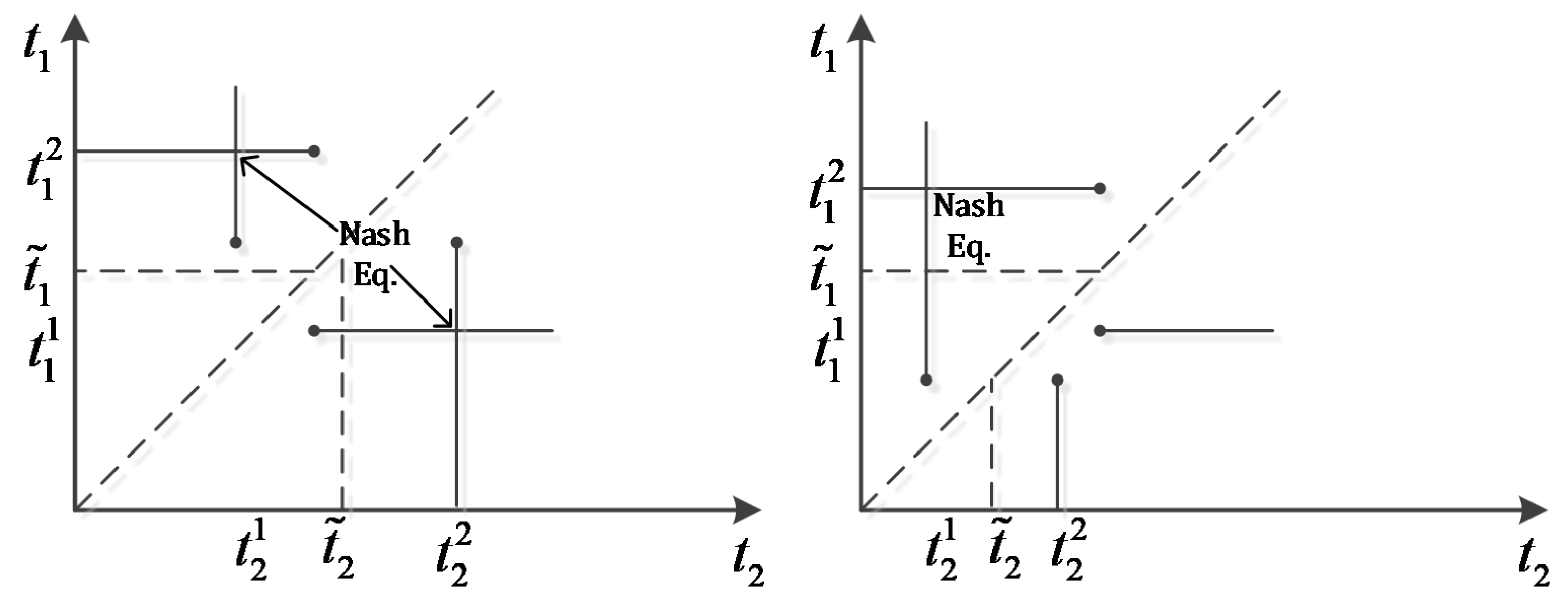
- (2)
- Iforor, then there exist two Nash equilibriaand.
- (3)
- Ifor, then there exists a unique Nash equilibrium.
3. Results
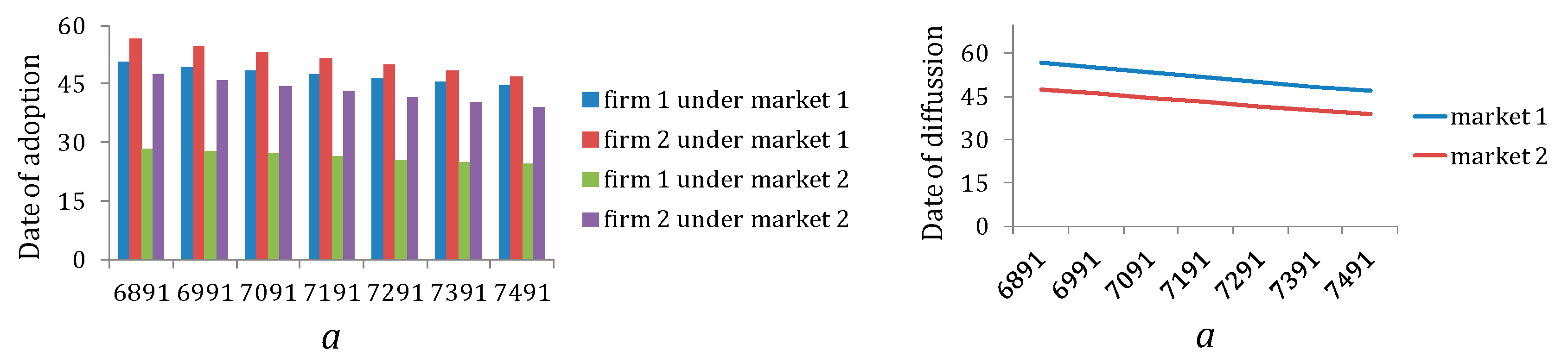
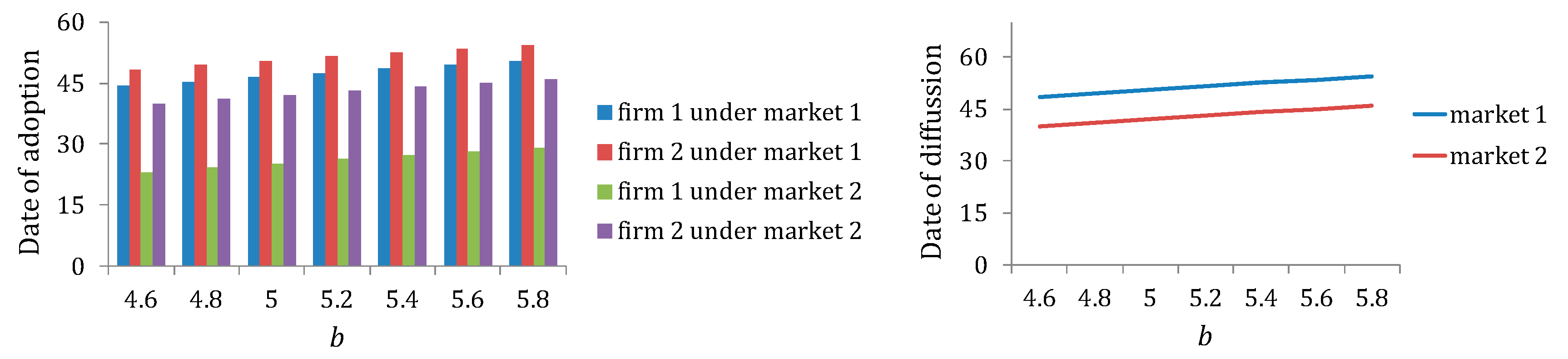
3.1. The Effect of Output Market
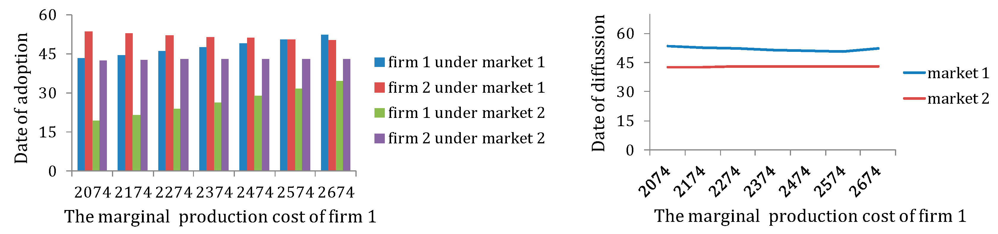
3.2. The Effect of Production Cost
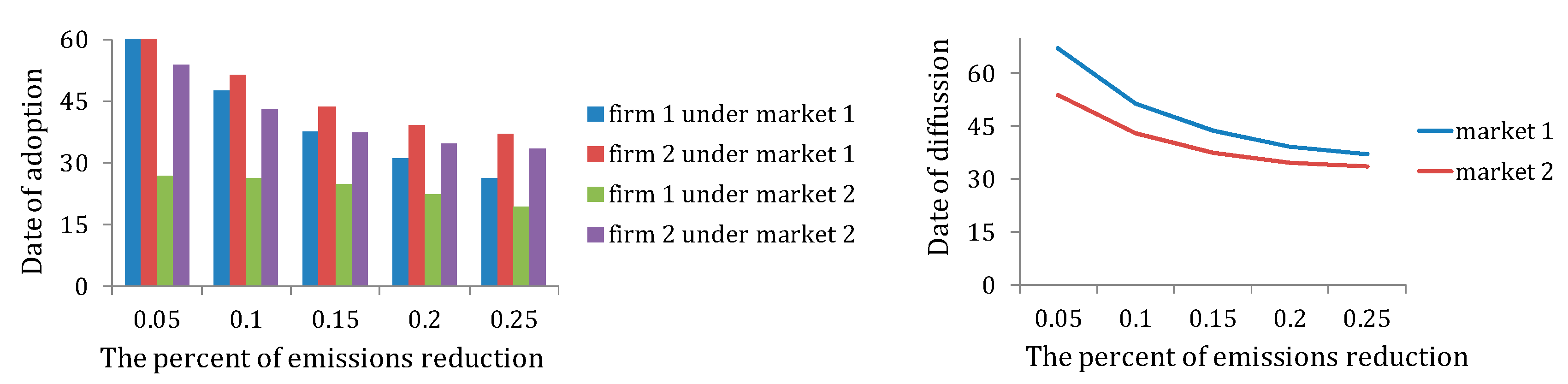
3.3. The Effect of Emissions Reduction Target
4. Discussion
4.1. Changes in Social Welfare
4.2. Comparison with Related Studies
4.3. Limitations and Further Research
5. Conclusions
Author Contributions
Funding
Conflicts of Interest
Appendix A. The Solution Process of in the Absence of Environmental Policy
Appendix B. The Results in the Perfectly Competitive Permits Market
Appendix C


References
- IPCC. Climate Change: The Physical Science Basis; Cambridge University Press: New York, NY, USA, 2007. [Google Scholar]
- Montero, J.P. Market power in pollution permit markets. Energy J. 2009, 30, 115–142. [Google Scholar] [CrossRef]
- Eyckmans, J.; Hagem, C. The European Union’s potential for strategic emissions trading through permit sales contracts. Resour. Energy Econ. 2011, 33, 247–267. [Google Scholar] [CrossRef]
- Min, X.J.; Dong, X.Y.; Zi, Y.C.; Pu, Y.N. Market power in auction and efficiency in emission permits allocation. J. Econ. Manag. 2016, 183, 576–584. [Google Scholar]
- Hintermann, B. Market power in emission permit markets: Theory and evidence from the EU-ETS. Environ. Resour. Econ. 2017, 66, 1–24. [Google Scholar] [CrossRef]
- Dickson, A.; Mackenzie, I.A. Strategic trade in pollution permits. J. Environ. Econ. Manag. 2018, 87, 94–113. [Google Scholar] [CrossRef]
- Hahn, R.W. Market power and transferable property rights. Q. J. Econ. 1984, 99, 753–765. [Google Scholar] [CrossRef]
- Westskog, H. Market power in a system of tradeable CO2 quotas. Energy J. 1996, 17, 85–104. [Google Scholar] [CrossRef]
- Misiolek, W.S.; Elder, H.W. Exclusionary manipulation of markets for pollution rights. J. Environ. Econ. Manag. 1989, 16, 156–166. [Google Scholar] [CrossRef]
- Malik, A.S. Further results on permit markets with market power and cheating. J. Environ. Econ. Manag. 2002, 44, 1–390. [Google Scholar] [CrossRef]
- Hintermann, B. Market power, permit allocation and efficiency in emission permit markets. Environ. Resour. Econ. 2011, 49, 327–349. [Google Scholar] [CrossRef]
- Hintermann, B. Pass-through of CO2 emission costs to hourly electricity prices in Germany. J. Assoc. Environ. Resour. Econ. 2016, 3, 857–891. [Google Scholar] [CrossRef]
- Tanaka, M.; Chen, Y. Market power in emissions trading: Strategically manipulating permit price through fringe firms. Appl. Energy 2012, 96, 203–211. [Google Scholar] [CrossRef]
- Haita, C. Endogenous market power in an emissions trading scheme with auctioning. Resour. Energy Econ. 2014, 37, 253–278. [Google Scholar] [CrossRef]
- Amundsen, E.S.; Bergman, L. Green certificates and market power on the Nordic power market. Energy J. 2012, 33, 101–118. [Google Scholar] [CrossRef]
- Zhang, Z. Carbon emissions trading in China: The evolution from pilots to a nationwide scheme. Clim. Policy 2015, 15, S104–S126. [Google Scholar] [CrossRef]
- Wrake, M.; Myers, E.; Mandell, S.; Holt, C.; Burtraw, D. Pricing Strategies Under Emissions Trading: An Experimental Analysis; RFF Discussion Paper: Washington, DC, USA, 2008; pp. 8–49. [Google Scholar]
- Dormady, N.C. Carbon auctions, energy markets & market power: An experimental analysis. Energy Econ. 2014, 44, 468–482. [Google Scholar]
- Noah, D. Carbon auction revenue and market power: An experimental analysis. Energies 2016, 9, 897–917. [Google Scholar]
- Álvarez, F.; André, F.J. Auctioning versus grandfathering in cap-and-trade systems with market power and incomplete information. Environ. Resour. Econ. 2015, 62, 873–906. [Google Scholar] [CrossRef]
- D’amato, A.; Valentini, E.; Zoli, M. Tradable quota taxation and market power. Energy Econ. 2017, 63, 248–252. [Google Scholar] [CrossRef]
- Montero, J.P. Permits, standards, and technology innovation. J. Environ. Econ. Manag. 2002, 44, 23–44. [Google Scholar] [CrossRef]
- Montero, J.P. Market structure and environmental innovation. J. Appl. Econ. 2002, 5, 293–325. [Google Scholar] [CrossRef]
- Storrosten, H.B. Incentives to Invest in Abatement Technology: A Tax versus Emissions Trading under Imperfect Competition; Discussion Papers no. 606; Statistics Norway, Research Department: Oslo, Norway, 2010. [Google Scholar]
- Zhou, P.; Wang, M. Carbon dioxide emissions allocation: A Review. Ecol. Econ. 2016, 125, 47–59. [Google Scholar] [CrossRef]
- Narassimhan, E.; Gallagher, K.S.; Koester, S.; Alejo, J.R. Carbon pricing in practice: A review of existing emissions trading systems. Clim. Policy 2018, 18, 967–991. [Google Scholar] [CrossRef]
- André, F.J.; Arguedas, C. Technology adoption in emission trading programs with market power. Energy J. 2018, 39, 145–174. [Google Scholar] [CrossRef]
- Wang, X.; Zhang, X.B.; Zhu, L. Imperfect market, emissions trading scheme, and technology adoption: A case study of an energy-intensive sector. Energy Econ. 2019, 81, 142–158. [Google Scholar] [CrossRef]
- Rogge, K.S.; Schneider, M.; Hoffmann, V.H. The innovation impact of the EU Emission Trading System—Findings of company case studies in the German power sector. Ecol. Econ. 2011, 70, 513–523. [Google Scholar] [CrossRef]
- Wang, X.; Zhu, L.; Fan, Y. Transaction costs, market structure and efficient coverage of emissions trading scheme: A microlevel study from the pilots in China. Appl. Energy 2018, 220, 657–671. [Google Scholar] [CrossRef]
- Rana, M.M.; Li, L.; Su, S.W. An adaptive-then-combine dynamic state estimation considering renewable generations in smart grids. IEEE J. Sel. Areas Commun. 2016, 34, 3954–3961. [Google Scholar] [CrossRef]
- Rana, M.M. Modelling the microgrid and its parameter estimations considering fading channels. IEEE Access 2017, 5, 10953–10958. [Google Scholar] [CrossRef]
- Rana, M.M.; Li, L.; Su, S.W.; Xiang, W. Consensus-based smart grid state estimation algorithm. IEEE Trans. Ind. Inf. 2017, 14, 3368–3375. [Google Scholar] [CrossRef]
- Rana, M.M. Architecture of the internet of energy network: An application to smart grid communications. IEEE Access 2017, 5, 4704–4710. [Google Scholar] [CrossRef]
- Rana, M.M.; Xiang, W.; Wang, E.; Li, X.H. Monitoring the smart grid incorporating turbines and vehicles. IEEE Access 2018, 6, 45485–45492. [Google Scholar] [CrossRef]
- Rana, M.M.; Xiang, W.; Wang, E. Iot-based state estimation for microgrids. IEEE Internet Things J. 2018, 5, 1345–1346. [Google Scholar] [CrossRef]
- Rana, M.M.; Xiang, W.; Wang, E. Smart grid state estimation and stabilisation. Int. J. Electr. Power Energy Syst. 2018, 102, 152–159. [Google Scholar] [CrossRef]
- Reinganum, J.F. On the diffusion of new technology: A game theoretic approach. Rev. Econ. Stud. 1981, 48, 395–405. [Google Scholar] [CrossRef]
- Coria, J. Taxes, permits, and the diffusion of a new technology. Resour. Energy Econ. 2009, 31, 249–271. [Google Scholar] [CrossRef]
- Sanin, M.E.; Zanaj, S. A note on clean technology adoption and its influence on tradeable emission permits prices. Environ. Resour. Econ. 2011, 48, 561–567. [Google Scholar] [CrossRef]
- Lecuyer, O.; Quirion, P. Can uncertainty justify overlapping policy instruments to mitigate emissions? Ecol. Econ. 2013, 93, 177–191. [Google Scholar] [CrossRef]
- Li, Y.; Zhu, L. Cost of energy saving and CO2 emissions reduction in China’s iron and steel sector. Appl. Energy 2014, 130, 603–616. [Google Scholar] [CrossRef]
- Guo, J.X.; Zhu, L. Optimal timing of technology adoption under the changeable abatement coefficient through R & D. Comput. Ind. Eng. 2016, 96, 216–226. [Google Scholar]
- Zhu, L.; Zhang, X.B.; Li, Y.; Wang, X.; Guo, J. Can an emission trading scheme promote the withdrawal of outdated capacity in energy-intensive sectors? A case study on China’s iron and steel industry. Energy Econ. 2017, 63, 332–347. [Google Scholar] [CrossRef]
- Khanna, M.; Zilberman, D. Incentives, precision technology and environmental protection. Ecol. Econ. 1997, 23, 25–43. [Google Scholar] [CrossRef]
- Frondel, M.; Horbach, J.; Rennings, K. End-of-pipe or cleaner production? An empirical comparison of environmental innovation decisions across OECD countries. Bus. Strat. Environ. 2007, 16, 571–584. [Google Scholar] [CrossRef]
- Hammar, H.; Löfgren, A. Explaining adoption of end-of-pipe solutions and energy-saving technologies—Determinants of firms’ investments for reducing emissions to air in four sectors in Sweden. Energy Policy 2010, 38, 3644–3651. [Google Scholar] [CrossRef]


| Adoption Dates | The Profit of Firm 1 | The Profit of Firm 2 |
|---|---|---|
| Parameters | Dimension | Description | Value | Source |
|---|---|---|---|---|
| Parameters in linear inverse demand function | 7191 | [44] | ||
| 5.2 | ||||
| (yuan/tSteel) | Firm 1’s production cost coefficient | 2374 | ||
| (yuan/tSteel) | Firm 2’s production cost coefficient | 3543 | ||
| (tSteel/tCO2) | Firm 1’s initial emissions intensity | 0.6 | ||
| (tSteel/tCO2) | Firm 2’s initial emissions intensity | 0.47 | ||
| (tSteel/tCO2) | Emissions intensity of the new technology | 0.8 | Given | |
| (million yuan) | The parameter of investment cost | 1 | Given | |
| The diffusion rate | 0.038 | [39] | ||
| Percentage of emissions reductions | 0.1 | Given | ||
| The discount rate | 0.05 | Given |
| 6891 | 6991 | 7091 | 7192 | 7291 | 7391 | 7491 | |
|---|---|---|---|---|---|---|---|
| 414 | 426 | 426 | 426 | 426 | 425 | 425 | |
| 48,642 | 46,486 | 45,767 | 45,049 | 44,331 | 43,614 | 42,898 | |
| −71,379 | −75,291 | −79,222 | −83,375 | −87,785 | −92,265 | −96,938 | |
| 120,435 | 122,203 | 125,415 | 128,850 | 132,542 | 136,304 | 140,261 | |
| 0 | 0 | 0 | 0 | 0 | 0 | 0 | |
| 83,220 | 83,220 | 83,220 | 83,220 | 83,220 | 83,220 | 83,220 | |
| −8489 | −9502 | −10,635 | −11,847 | −13,250 | −14,763 | −16,430 | |
| 91,709 | 92,722 | 93,855 | 95,067 | 96,470 | 97,983 | 99,651 |
| 4.6 | 4.8 | 5.0 | 5.2 | 5.4 | 5.6 | 5.8 | |
|---|---|---|---|---|---|---|---|
| 377 | 393 | 409 | 426 | 442 | 459 | 475 | |
| 50,925 | 48,803 | 46,851 | 45,049 | 43,380 | 41,831 | 40,389 | |
| −110,840 | −100,390 | −91,363 | −83,375 | −76,399 | −70,255 | −64,805 | |
| 162,142 | 149,586 | 138,623 | 128,850 | 120,220 | 112,545 | 105,669 | |
| 0 | 0 | 0 | 0 | 0 | 0 | 0 | |
| 94,075 | 90,155 | 86,549 | 83,220 | 80,138 | 77,276 | 74,611 | |
| −15,819 | −14,281 | −12,982 | −11,847 | −10,915 | −9992 | −9239 | |
| 109,894 | 104,440 | 99,531 | 95,067 | 91,053 | 87,268 | 83,850 |
© 2019 by the authors. Licensee MDPI, Basel, Switzerland. This article is an open access article distributed under the terms and conditions of the Creative Commons Attribution (CC BY) license (http://creativecommons.org/licenses/by/4.0/).
Share and Cite
Zeng, B.; Zhu, L. Market Power and Technology Diffusion in an Energy-Intensive Sector Covered by an Emissions Trading Scheme. Sustainability 2019, 11, 3870. https://doi.org/10.3390/su11143870
Zeng B, Zhu L. Market Power and Technology Diffusion in an Energy-Intensive Sector Covered by an Emissions Trading Scheme. Sustainability. 2019; 11(14):3870. https://doi.org/10.3390/su11143870
Chicago/Turabian StyleZeng, Bingxin, and Lei Zhu. 2019. "Market Power and Technology Diffusion in an Energy-Intensive Sector Covered by an Emissions Trading Scheme" Sustainability 11, no. 14: 3870. https://doi.org/10.3390/su11143870
APA StyleZeng, B., & Zhu, L. (2019). Market Power and Technology Diffusion in an Energy-Intensive Sector Covered by an Emissions Trading Scheme. Sustainability, 11(14), 3870. https://doi.org/10.3390/su11143870