Applying Machine Learning and Statistical Approaches for Travel Time Estimation in Partial Network Coverage

Abstract

The objective of this study is to estimate the real time travel times on urban networks that are partially covered by moving sensors. The study proposes two machine learning approaches; the random forest (RF) model and the multi-layer feed forward neural network (MFFN) to estimate travel times on urban networks which are partially covered by moving sensors. A MFFN network with three hidden layers was developed and trained using the back-propagation learning algorithm, and the neural weights were optimized using the Levenberg–Marquardt optimization technique. A case study of an urban network with 100 links is considered in this study. The performance of the proposed models was compared to a statistical model, which uses the empirical Bayes (EB) method and the spatial correlation between travel times. The models’ performances were evaluated using data generated from VISSIM microsimulation model. Results show that the machine learning algorithms, e.g., RF and ANN, achieve average improvements of about 4.1% and 2.9% compared with the statistical approach. The RF, MFFN, and the statistical approach models correctly predict real time travel times with estimation accuracies reaching 90.7%, 89.5%, and 86.6% respectively. Moreover, results show that at low moving sensor penetration rate, the RF and MFFN achieve higher estimation accuracy compared with the statistical approach. At probe penetration rate of 1%, the RF, MFFN, and the statistical approach models correctly predict real time travel times with estimation accuracy of 85.6%, 84.4%, and 80.9% respectively. Furthermore, the study investigated the impact of the probe penetration rate on real time neighbor links coverage. Results show that at probe penetration rates of 1%, 3%, and 5%, the models cover the estimation of real time travel times on 73.8%, 94.8%, and 97.2% of the estimation intervals.

1. Introduction

Accurate travel time estimation and prediction are important for intelligent transportation systems (ITS), as it enables transportation system operators to efficiently manage transportation networks by displaying the current transportation network conditions on variable message signs (VMS), and directing drivers to less congested routes. Moreover, accurate estimations allow road users to better schedule their trips and select their routes.

Because of its stochastic nature, travel time estimation is challenging, especially in urban road networks. The uncertainty in urban link travel times can be attributed to the traffic demand fluctuations, the existence of traffic controls, and stochastic nature of traffic flow at signalized intersections. In the past, traffic data has been usually collected using point detectors, such as loop detectors, which is why numerous travel time estimation models were developed based on the data obtained from such detectors [1,2]. However, the large-scale utilization of point detectors has been limited, mainly because installing and maintaining point detectors that can sufficiently cover large urban networks that comes at a high cost. More recently, moving traffic sensors—e.g., probe vehicles—are being used extensively to collect traffic data which also includes measured travel times. Newer models of travel time estimation that depend on moving traffic sensor data have also been developed [3,4,5,6].

In general, the probe penetration rate of moving sensors is limited, as it mainly relies on GPS equipped public transportation vehicles and taxi fleets. The limited penetration rate limits the availability of data, both temporally and spatially, leading to a partial coverage of the traffic network. In such cases, the ITS either relies on historical data or adopts travel time estimation models. Such models can utilize the spatial correlation between network links travel times to estimate links travel times that are not covered by moving sensors [7,8,9,10,11].

Most current moving sensor-based models used for real time traffic prediction on partially covered networks require both historical and real time data. Relying on historical traffic data can limit the accuracy of the prediction models especially in handling highly dynamic traffic conditions. In this paper, a random forest (RF) and a multi-layer feed forward neural network (MFFN) models are proposed for the estimation of the real time travel times on networks that are partially covered by moving sensors. The proposed models utilize minimal real time traffic data—e.g., travel times—on spatially correlated neighbor links obtained from probe vehicles. The accuracy of the proposed models are compared with the statistical model developed by [10] which utilizes both link historical travel time and neighbor links real time travel times in estimating the real time travel time on the target link. Neural network modeling approach is more robust compared with the statistical-regression modelling as building the structure of the model and calibrating its parameters is done by utilizing the data. RF models, which are an ensemble learning technique, predict the results based on a voting mechanism, which may have higher prediction accuracy than artificial neural nets (ANN) as a group of predictors can perform better than a single predictor. Furthermore, both RF and ANN require no assumption about the input variables or the error structure, and the issue of multicollinearity can be neglected. Moreover, this paper discusses the issue of probe vehicle market penetration rate and investigates its impact on the estimation accuracy utilizing the proposed RF and ANN estimation models.

2. Literature Review

In the recent years, estimating and predicting of travel time in urban road networks have been extensively studied. The use of probe vehicles as moving sensors for collecting traffic data have been advocated in numerous previous work [3,10,11,12]. Generally, travel time estimation or prediction techniques are classified into model-based approaches, e.g., mathematical models, and data-driven approaches, e.g., regression models. Liu and Ma [13] proposed a model that traces a virtual vehicle path through multiple intersections to estimate arterial travel times. The model uses high-resolution data of vehicles actuation over loop detector and signal phases. Jula et al. [14] proposed a mathematical-model to predict real time travel times on dynamic road network. The study uses a Kalman filter with a predictor corrector in travel time prediction. Li et al. [1] developed a traffic theory time-based algorithm to estimate links travel using traffic data—e.g., vehicle speeds and headways series—measured at upstream and downstream detectors.

Unlike the model-based approach that required extensive traffic data collection, the data-driven approach can deal with low-resolution data obtained by moving sensors. Examples of such approach involve statistical models [10,12], neural network models [3], pattern recognition models [15], and Random Forest model. Jenelius and Koutsopoulos [12] proposed a statistical-model in order to estimate travel times on road network using vehicle trajectories obtained from probe vehicles. The model uses travel time correlation between network segments for the observations from the same vehicle trajectory. Elesawey and Sayed [10] proposed a statistical approach to estimate travel times on urban network using neighbor link travel times obtained from probe vehicles. The proposed model used the spatial correlation between link travel times. The study gave the term ‘neighbor links’ to links located in the same area type, having similar characteristics, whose travel times are correlated. Spatial correlation are found between link travel times and their link neighbors within the local traffic impact area [8]. Zheng and Van Zuylen [3] proposed a neural network with a single hidden layer to estimate travel time on a link based on a partial traffic data collected on the link using probe vehicles. Zhang et al. [15] proposed a pattern matching method for travel time prediction on expressways using data obtained from probe vehicles. The method employed a large-scale spatiotemporal traffic pattern matching for multi-step travel time forecasting.

Spatial travel time correlation has been broadly discussed in the literature. Chen et al. [8] found spatial correlation between link travel time and its neighbor links located within the impact area. The study considered spatial correlation between links travel time within a topological distance which is quantified as the number of links between the target links. El Esawey and Sayed [10] found spatial correlation between links travel times. The study utilized the spatial travel time correlations in identifying link neighbors. Empirical studies based on real data found spatial travel time correlation between neighbor links [11] and strong correlation were found on adjacent links [16]. Jenelius and Koutsopoulos [12] found spatial travel time correlation between the network links based on empirical data. The study assumed that each link travel time is influenced by its nearest neighbors. Zeng et al. [17] found that the spatial travel time correlation between links increases if they are connected, or if they have similar movement direction and traffic control type.

Despite the advantages of using moving sensors for collecting real time traffic data, the issue of adopting a probe’s penetration rate that provides sufficient network coverage is raised. Probe penetration rate refers to the use of a portion of network traffic—e.g., taxi fleets—as a source of collecting real time travel time data. Previous studies showed that the performance of probe-based traffic estimation models can be affected by the probe penetration rate. Moreover, network links coverage and link neighbor coverage are significantly impacted by the probe penetration rate in urban network [10,11,18]. Therefore, this paper also extends the proposed methodology of travel time estimation using RF and ANN to evaluate the proposed models performance at different probe penetration rates.

3. Methodology

3.1. Neighbor Link Allocation

The concept of ‘neighbor links’ was proposed in the literature [8,10] to characterize travel times relation between links in urban road networks. The term ‘neighbor links’ is used to specify links that located within the same area type, have similar characteristics, and spatial correlations exist between their travel times. Neighbor links can be any link in the urban network, e.g., proceeding or succeeding link, parallel of intersecting links. Specifying neighbor links to be in the same area type ensures the neighbor links are subjected to similar traffic condition. Moreover, neighbor links are specified to have similar vehicle entry/exit movement direction as the statistical properties of link travel times distribution were shown to be affected by the direction at which vehicles enter/exit the links [19]. Traffic attributes as left and right turns at intersections were found to significantly affect links travel times [12].

Previous studies investigated the impact of the correlation threshold in identifying link neighbors on both the estimation accuracy and the number of identified link neighbors [11,20]. The studies found that increasing the correlation cut-off value for identifying link neighbors decreases the number of the identified link neighbors to appoint where no neighbor can be identified. Moreover, an increase in the correlation threshold from 0.4 to 0.7 did not show a significant increase in the accuracy of the statistical model. Therefore, in this study, a correlation threshold of 0.4 is used to identify links neighbors. It is noteworthy that the Pearson correlation is used as an input dimension reduction for the proposed models as the degree of the input relevance to the output can impact the estimation accuracy. As well, increasing the input dimension may increase the training algorithm convergence problems and increase the computational cost [21].

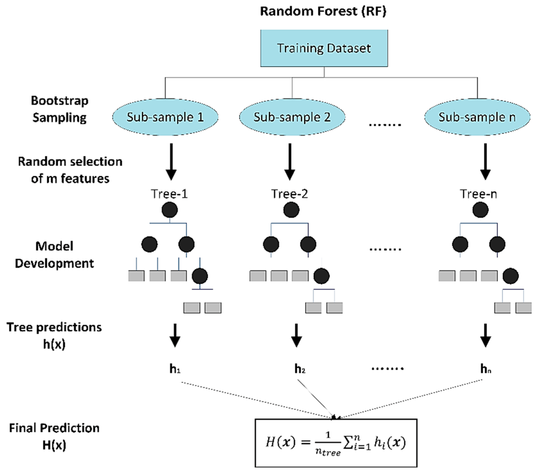
3.2. Random Forest Model

Random forest (RF) model is considered as an ensemble learning technique at which the prediction is dependent on a group of trees [22]. Unlike regression tree, which depends on the individual tree structure, the final prediction result in RF is based on a voting mechanism where each decision tree in the forest has a vote, and the final prediction is the average of votes as presented in Equation (1).

$$H\left(\mathit{x}\right)=\frac{1}{n_{tree}}{{\displaystyle \sum }}_{i=1}^n{h}_i\left(\mathit{x}\right)$$

(1)

where H(.) is the final prediction results, n_tree is the number of trees in the forest, h_i(.) is the prediction result of the i^th tree, and x is the input vector. Each tree in the RF model is an expert of regression with a certain set of features, e.g., input variables. To address the issue of correlation and to increase the variability between the decision trees in RF, each decision tree is built from a different subset of the training dataset, and the input variables is randomly selected and used to determine each tree split [23]. In the RF, the bootstrap sampling is implemented which enables the computation of the error using the unused subset of the training dataset. As the model is based on multiple trees, the prediction is more stable and less sensitivities to the input data outlier [24].

Figure 1 illustrates the RF model. RF model builds a forest with n_tree number of trees. Each tree is generated by a random subset of m_try input features/variables. Each tree is an expert with its subset features. Each tree outputs the prediction at one of its end leaves and the final prediction of the forest is the average of the prediction of each tree. Increasing the number of input features m_try that generates each tree in the forest may increase the strength of the induvial trees, but may increase the correlation between them. The prediction accuracy of the RF increases as the strength of trees increase but decreases as the correlation between them increase [22]. Therefore, a trade-off between the strength and correlation should be considered to improve the RF prediction performance.

Furthermore, increasing the number of trees n_tree in the FR models improves and stabilizes the performance of the RF to a point where no significant performance improvement can be obtained, and would only increase the computational cost [25]. In this study, the analysis of the developed RF models showed that the performance of the models is stable and no significant performance gain by increasing the number of trees n_tree to be more than 2000 trees in each RF model. Moreover, the performance of the RF models was tested using a different number of input features m_try, and the optimal performance was obtained at a number of input features m_try up to 3. The results of the RF presented in this paper is the average of 10 RF developed by different seeds. The RF models were developed using R-software.

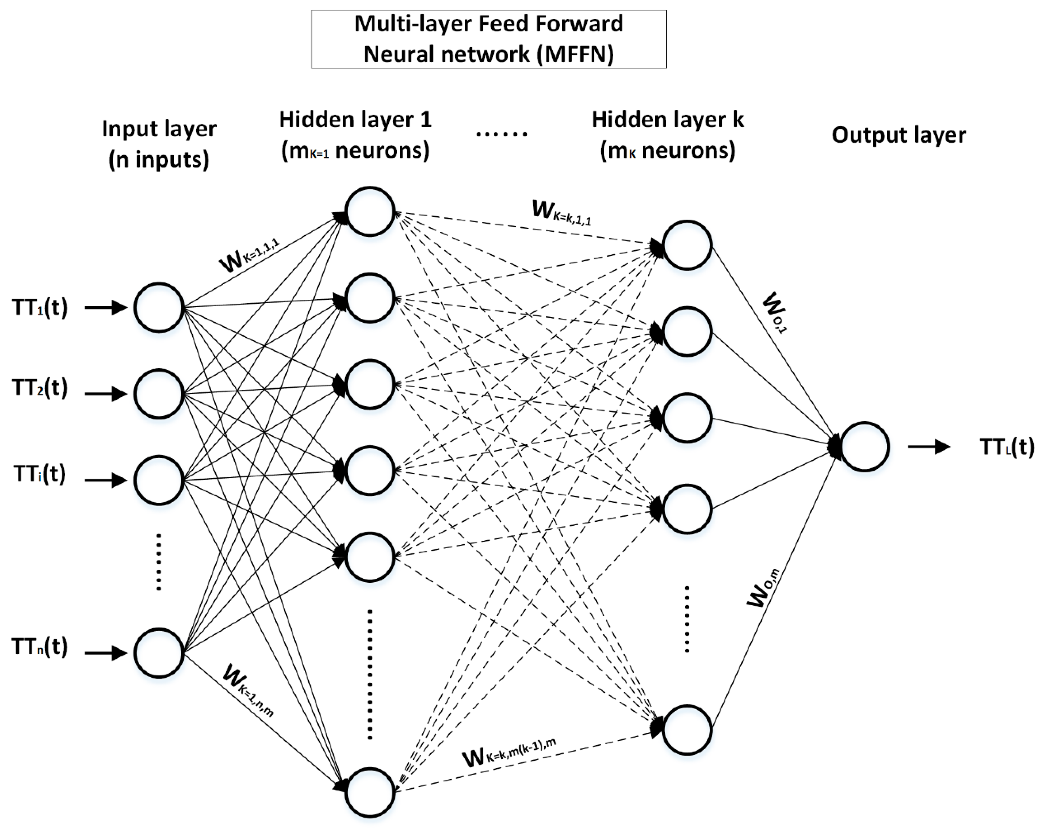
3.3. Artificial Neural Network Model

Artificial neural network (ANN) is inspired from the functional aspect of the biological neural system that constitutes brains. The strength of an ANN arises from its ability to learn from demonstrations of examples. ANN is rapidly spreading in many research disciplines in natural and applied science [3,26,27].

ANN performs computations through a structured architecture of interconnected groups of artificial neurons. The multi-layer feed forward neural network (MFFN) is popular and it consists of interconnected several layers of neurons, e.g., input layer, hidden layer(s), and the output layer [28]. The main component of the neural network is the neurons. The input neurons (i.e., neurons in the input layers) contain the explanatory variables (e.g., the link neighbors travel times). The output neuron(s), i.e., in the output layer, contains the dependent variable(s), e.g., the predicted travel time on the target link. The hidden neurons which are in the hidden layer(s) connect and transfer the information or signal from the input neurons to the output neuron(s). In the feed forward network, the information or signal is propagating in the network from the input neuron(s) to the output neuron(s) in a single direction through the links that connect the neurons, i.e., there is no loop in the network. The links have numeric weights $\mathit{w}$ which are beneficial in representing the effect of synapses by modulating the weights of the input information/signals. The weights $\mathit{w}$ can be adjusted using a learning algorithm to learn the relationship in the data. The nonlinear effect of the neurons is represented by the transform function at each neuron. The weights are multiplied by the input values from the previous neurons and are summed up at each node. Then the information/signal is propagated to the next neurons by the transfer function.

In this study, multi-layer feed forward neural networks (MFFN) were constructed to estimate target links travel times based on neighbor links’ travel time data. The neural networks were trained using the back-propagation learning algorithm which provides a procedure for updating the weights $\mathit{w}$ in the neural network to correctly predict the output in the training data set. The Levenberg–Marquardt optimization technique [29,30] was used to update the weights $\mathit{w}$ in the back-propagation algorithm. The Levenberg–Marquardt optimization technique was to possibly avoid the overfitting of the network. Moreover, the Levenberg–Marquardt provides a fast convergence even for a large neural network that contains hundreds of weights. The back-propagation algorithm involves the feed forward of input information/signal, and back-propagation computation of error and adjusts the weight accordingly to minimize the error.

Figure 2 illustrates the structure of the multi-layer feed forward neural network adopted in this study. Each of the neural-network developed in this study consist of n number of input neurons in the input layer of which each neuron represents a neighbor link of the target link Equation (2). Three dense hidden layers were developed in each neural network with 30 neurons in the first and second layers and 15 neurons in the third layer Equation (3). During the training process, a comparison of the prediction accuracy of the neural networks, while considering their complexity in terms of both the number of hidden layers and their neurons, is performed. Different numbers of hidden layers (e.g., 1, 2, and 3 hidden layer(s)) and different number of neurons in each layer (e.g., 5, 10, 15, 20, 25, 30, 35, and 40 neurons) with different transform function for neurons in each layer (e.g., logistic sigmoid and tangent sigmoid) are considered. Decreasing the hidden layers below two layers or the number of hidden neurons below 25 in the first two hidden layers were found to dramatically deteriorate the neural network performance. A previous study found that the performance of travel time estimation for a single layer neural network with 20 or 25 neurons is better than for the case with 10 or 15 neurons [3]. Using three hidden layers with 30 neurons in the first two hidden layers and 15 neurons in the third hidden layer with a logistic sigmoid transform function in the first two hidden layer and tangent sigmoid transform function in the third hidden layer and the output layer provided the best prediction accuracy, except for link ID 68 where the tangent sigmoid transfer function in all layers provided the best accuracy.

$$\mathit{X}\left(t\right)= \left[\begin{array}{c}{x}_1\left(t\right)\\ ⋮\\ x_i\left(t\right)\end{array}\right]$$

(2)

where $\mathit{X}\left(t\right)$ is the input vector during the time interval $t$, $x_i\left(t\right)$ is the average travel time on neighbor $i$ during the time interval $t$, where $i\in \left\{1, \dots , n\right\}$ is a discreet index for the number of neighbors of the target link. The hidden layers structure is defined as

$${\mathit{H}}_K\left(t\right)= \left[\begin{array}{c}{h}_{k,1}\left(t\right)\\ ⋮\\ h_{k,m}\left(t\right)\end{array}\right]=\left[\begin{array}{c}\phi \left({\displaystyle \sum }_{j=1}^N{w}_{k,1,j}{x}_j\left(t\right)+b_{k,1}\right)\\ ⋮\\ \phi \left({\displaystyle \sum }_{j=1}^N{w}_{k,m,j}{x}_j\left(t\right)+b_{k,m}\right)\end{array}\right].$$

(3)

where $H_K\left(t\right)$ is the $k^{th}$ hidden layer in the neural network, $h_{k,m}\left(t\right)$ is the value of the $m^{th}$ hidden neuron in $k^{th}$ hidden layer during the time interval $t$, where $m$ is a discreet index for the number of neurons in each layer, and $k\in \left\{1, 2,3\right\}$ is a discrete index for the number of hidden layers. The $w_{k,m,j}$ is the weight connecting the $j^{th}$ input from the previous layer to the $m^{th}$ hidden neuron in the $k^{th}$ hidden layer, $b_{k,m}$ is the bias value for the $m^{th}$ hidden neuron in $k^{th}$ hidden layer, and $\phi (.)$ is the transfer function. The transfer functions have several forms including the logistic sigmoid Equation (4) and the hyperbolic tangent sigmoid Equation (5).

$$\phi \left(x\right)= \frac{1}{1+e^{-x}}$$

(4)

$$\phi \left(x\right)= \frac{1-e^{-2x}}{1+e^{-2x}}$$

(5)

The output layer in the neural network outputs the estimation of the travel time based on the neighbor links travel times, and it is in Equation (6) as

$$TT\left(t\right)=\phi \left({{\displaystyle \sum }}_{j=1}^m{w}_j{h}_{3,j}\left(t\right)+b\right)$$

(6)

where $TT\left(t\right)$ is the target link travel time estimation during the time interval $t$, $w_j$ is the weight connecting the $j^{th}$ hidden neuron in the third hidden layer with the output neuron, $h_{3,j}\left(t\right)$ is the value of the $j^{th}$ hidden neuron in the third hidden layer during the time interval $t$, $b$ is the output neuron bias, and $\phi (.)$ is the transfer function. The models of the neural network were developed using the MATLAB.

3.4. Statistical Model

Different from the machine learning (ML) approaches of RF and ANN, El Esawey and Sayed [10] proposed a statistical model for real time travel time estimation on network that are partially covered by moving sensors, using an empirical Bayes (EB) fusion of link historical travel time and real time travel times from neighbor links. The proposed approach was implemented in several previous studies [11,20,31]. A brief description of the methodology is presented in the following.

The methodology uses two sources of data for the real time travel time estimation on links not covered by sensors. The first source is the link historical travel time, and the second source is the real time travel time on links neighbors. Let $x_{hl}$ represents the average historical travel time on link $l$ during a time interval $t$, $x_{rn}$ represents the estimation of the average real time travel time on link $l$ using travel times of neighbor links $n$ during a time interval $t$, and $\widehat{x}=f\left(x_{rn}, x_{hl}\right)$ represents the best estimate of real time average travel time on link $l$ during $t$. The best estimation of the link real time travel time $\widehat{x}$ of a link not covered by sensors can be computed through a data fusion between link historical travel time $\left(x_{hl}\right)$ and the estimation of the average real time travel time link $l$ using travel times of neighbor links $n$ during $t$ $\left(x_{rn}\right)$ as in Equation (7):

$$\widehat{x}=\alpha .x_{rn}+\left(1-\alpha \right).x_{hl}$$

(7)

where $\alpha \in \left[0,1\right]$ is the weight for $x_{rn}$, $\left(1-\alpha \right)$ is the weight for $x_{hl}$. The weight $\alpha$ can be estimated using the empirical Bayes (EB) approach which is considered one of the robust approaches for assigning weights using the observed data expectation and variance. The weight $\alpha$ can be computed as

$$\mathsf{\alpha }=\frac{1}{1+\frac{{\mathrm{Var}}_{({\mathrm{x}}_{rn})}}{{\mathrm{E}}_{\left({\mathrm{x}}_{\mathrm{rn}}\right)}}}.$$

(8)

where $Va{r}_{(x_{\begin{array}{c}rn\\ \end{array}})}$ and $E_{(x_{\begin{array}{c}rn\\ \end{array}})}$ are the variance and the expectation of the estimation of the average real time travel time on link $l$, respectively, using travel times of neighbor links $n$ during a time interval $t$. It is noteworthy that the weight $\alpha$ is dynamic and varies among intervals based on the expectation $E_{\left(x_{rn}\right)}$ and variance $Va{r}_{(x_{\begin{array}{c}rn\\ \end{array}})}$. The value of $x_{rn}$ can be estimated by constructing the relationship between the link travel time and link neighbor travel times. Regression models that relate link travel time with each link neighbor travel time were developed. The regression models are then combined using a weighting scheme to compute $x_{rn}$ as follow:

$${\mathrm{x}}_{\mathrm{rn}}={{\displaystyle \sum }}_{\mathrm{i}=1}^{\mathrm{n}}{\mathrm{w}}_{\mathrm{i}}.{\mathrm{x}}_{\mathrm{ri}}.$$

(9)

where $x_{ri}$ is the estimation of the travel time on link $l$ using travel times of neighbor links $i$ during a time interval $t$, where $i\in n$, $w_i$ is the weight for the estimation of the travel time on link $l$ using travel times of neighbor links $i$ during a time interval $t$. The $Va{r}_{(x_{\begin{array}{c}rn\\ \end{array}})}$ and $E_{\left(x_{rn}\right)}$ were obtained used the method of statistical differentiation as in Equation (10) and Equation (11)

$${\mathrm{E}}_{\left({\mathrm{x}}_{\mathrm{rn}}\right)}={\mathrm{x}}_{\mathrm{rn}}+\frac{{{\displaystyle \sum }}_{\mathrm{i}=1}^{\mathrm{n}}\frac{{\partial }^2{\mathrm{x}}_{\mathrm{rn}}}{\partial {\mathrm{x}}_{\mathrm{ri}}^2}.\mathrm{Var}\left({\mathrm{x}}_{\mathrm{ri}}\right)}{2}={\mathrm{x}}_{\mathrm{rn}}$$

(10)

$${\mathrm{Var}}_{({\mathrm{x}}_{\begin{array}{c}rn\\ \end{array}})}={{\displaystyle \sum }}_{\mathrm{i}=1}^{\mathrm{n}}{\left(\frac{\partial {\mathrm{x}}_{\mathrm{rn}}}{\partial {\mathrm{x}}_{\mathrm{ri}}}\right)}^2.\mathrm{Var}\left({\mathrm{x}}_{\mathrm{ri}}\right)={{\displaystyle \sum }}_{\mathrm{i}=1}^{\mathrm{n}}{({\mathrm{w}}_{\mathrm{i}})}^2.\mathrm{Var}{\left({\mathrm{x}}_{\mathrm{ri}}\right)}_{}$$

(11)

where $Var\left(x_{ri}\right)$ is the variance of the travel time estimation on link $l$ from neighbor link $i$ during $t$. Different weighting schemes $w_i$ can be used to combine the estimate from link neighbors. Weighting schemes can include the straight average weighting $w_i=1/n$, model variance weighting $w_i=\frac{1}{{\sigma }_i^2}/{\displaystyle \sum }_{i=1}^n\frac{1}{{\sigma }_i^2}$; exponent of model variance weighting $w_i=e^{\frac{1}{{\sigma }_i^2}}/{\displaystyle \sum }_{i=1}^n{e}^{\frac{1}{{\sigma }_i^2}}$; coefficient of determination weighting $w_i=R_i^2/{\displaystyle \sum }_{i=1}^n{R}_i^2$; correlation coefficient weighting $w_i=r_i/{\displaystyle \sum }_{i=1}^n{r}_i$; exponent of correlation coefficient weighting $w_i=e^{r_i}/{\displaystyle \sum }_{i=1}^n{e}^{r_i}$; and combined weighing approaches, e.g., combined correlation coefficient and exponent of model variance $w_i=r_i.e^{\frac{1}{{\sigma }_i^2}}/{\displaystyle \sum }_{i=1}^n{r}_i.e^{\frac{1}{{\sigma }_i^2}}$. Sensitivity analysis for the weighting schemes is conducted later in the paper. Different regression models were investigated including linear, exponential, power, and logarithmic models. The linear models outperformed the other models.

4. Models Application

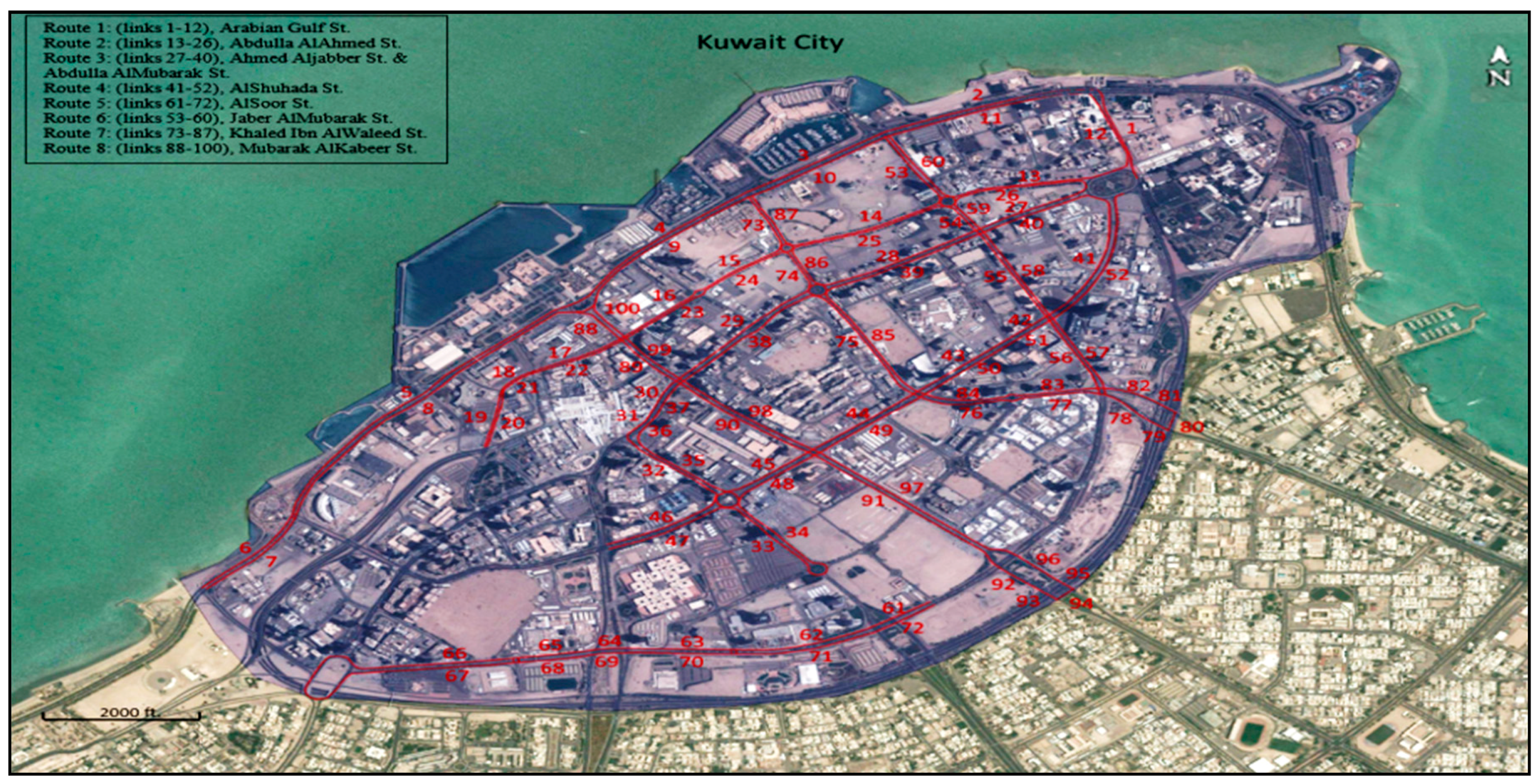
4.1. Urban Road Network

The urban road network of Kuwait City in the State of Kuwait, shown in Figure 3, is considered in this study. Kuwait City, the capital of Kuwait, is a central business district with considerable congestion during the peak hours. Kuwait City is a typical urban road network of two-way roads and signalized intersections at most of the intersections. The free flow speed on the links ranges from 60 to 80 km/h. A calibrated Vissim model of Kuwait City [11] is used to test different scenarios in this study. The Vissim model includes 100 links in Kuwait City, which are considered in the analysis.

4.2. Data Preparation

4.2.1. Travel Time Re-Sampling Process

A calibrated Vissim model of Kuwait City [11] is used to generate data in this study. The geometric design of the Kuwait City network was built in the Vissim model using a GIS map that represents accurate geometric of the streets. Traffic signals, priority rules, traffic conflict areas, and reduced speed areas were programmed in the model. The desired speeds on the links were programmed as the posted speed on each link. Travel time sections were programmed to measure link travel times including the signal delays. The original traffic demand level of the Vissim network model represents the pm peak traffic flow. Ten different demand levels were simulated as presented in

Table 1. Description of the training and testing dataset.

Training dataset: traffic demand levels as a percentage of the pm peak demand	60%, 65%, 70%, 80%, 90%, 100%, 105%
Testing (Validation) dataset: traffic demand levels as a percentage of the pm peak demand	75%, 85%, 95%
Simulation period for each demand level	60 min
Sampling interval	5 min

.

The network of the Kuwait City was resampled for a period of 75 minutes at different traffic demand levels. The warm-up period is considered as the first 15 min of the simulation run and therefore was discarded from the analysis. The data extraction process was conducted based on a sampling interval of 5 min (i.e., 12 time-interval in each hour), which is a broadly used sampling interval for probe vehicle travel time studies [10,19,32]. Link travel times were computed for each 5-min interval as the mean travel time of all vehicles traversing the link during each sampling interval. The simulation network model was used to generate data for 10 different scenarios of traffic demand during the pm peak period. The network was simulated for the original traffic demand level—e.g., 100% demand level—and for the demand levels of 60% to 105% with an increment of 5% demand levels. Moreover, three probe vehicle market penetration rates of 1%, 3%, and 5% were considered in the analysis. At each traffic demand level, link average travel times were computed for each sampling interval using the different probes penetration rates.

4.2.2. Data for Training and Testing

The simulated travel time data for the 10 demand levels were divided into two sets; the training dataset which consists of 7 demand levels (70% of the data), while the ramming dataset, e.g., 3 demand levels (30% of the data), was used as a testing (validation) dataset as shown in Table 1. A sampling interval of 5 min is used to compute links travel times (i.e., 12 time-intervals in each hour). Link travel times were computed for each 5-min interval as the mean travel time of all vehicles traversing the link during that interval. The training data set was used to train the three models, e.g., random forest (RF) model, artificial neural network (ANN) model, and the statistical model. The remaining set of the data, e.g., testing (validation) dataset, were used in the performance evaluation of the developed models. The training dataset consists of seven different demand levels, e.g., all the simulated traffic demand levels except 75%, 85%, and 95% of the traffic demand levels. As well, the simulated travel time data was used to conduct sensitivity analysis of the models’ performance and neighbor links coverage at the different probe penetration rates.

It is noteworthy that the random forest models and the artificial neural network models were developed based on link neighbor real time travel times, while the statistical model uses both link historical travel time and link neighbor real time travel times.

4.3. Performance Evaluation

The performance of the developed models was evaluated using the testing dataset (Table 1) using a performance indicator of the mean absolute percentage error (MAPE) Equation (12)

$$MAPE=\frac{100}{N}{{\displaystyle \sum }}_{i=1}^N\left|\frac{x_{true,i}-x_{est,i}}{x_{true,i}}\right|.$$

(12)

where $x_{true,i}$ is the true link travel time during the time interval $i$, $x_{est,i}$ is the estimation of the real time link travel time using data of neighbor links n during a time interval i, and N is the total number of observation in the testing dataset. Moreover, links coverage was evaluated at the three probes penetration rates of 1%, 3%, and 5%. Links coverage was computed as the percentage of the number of intervals at which the real time travel times are available for link neighbors during the total measurement Equation (13)

$$Lin{k}^{\prime }sCoverag{e}_l(\%)=\left({{\displaystyle \sum }}_{i=1}^N{I}_{l,i}\right)/N*100.$$

(13)

where N is the number of intervals considered in the evaluation, $i\in \left\{1,\dots ,N\right\}$, is a discrete index for the number of intervals, $I_{l,i}$, is a binary variable $I_{l,i} \in \left\{0,1\right\}$, where $I_{l,i}$ equals 0 when there are no neighbors identified for link $l$ during the interval $i$, and equals to 1 where there is at least one neighbor identified for link $l$, during the interval $i$.

5. Results

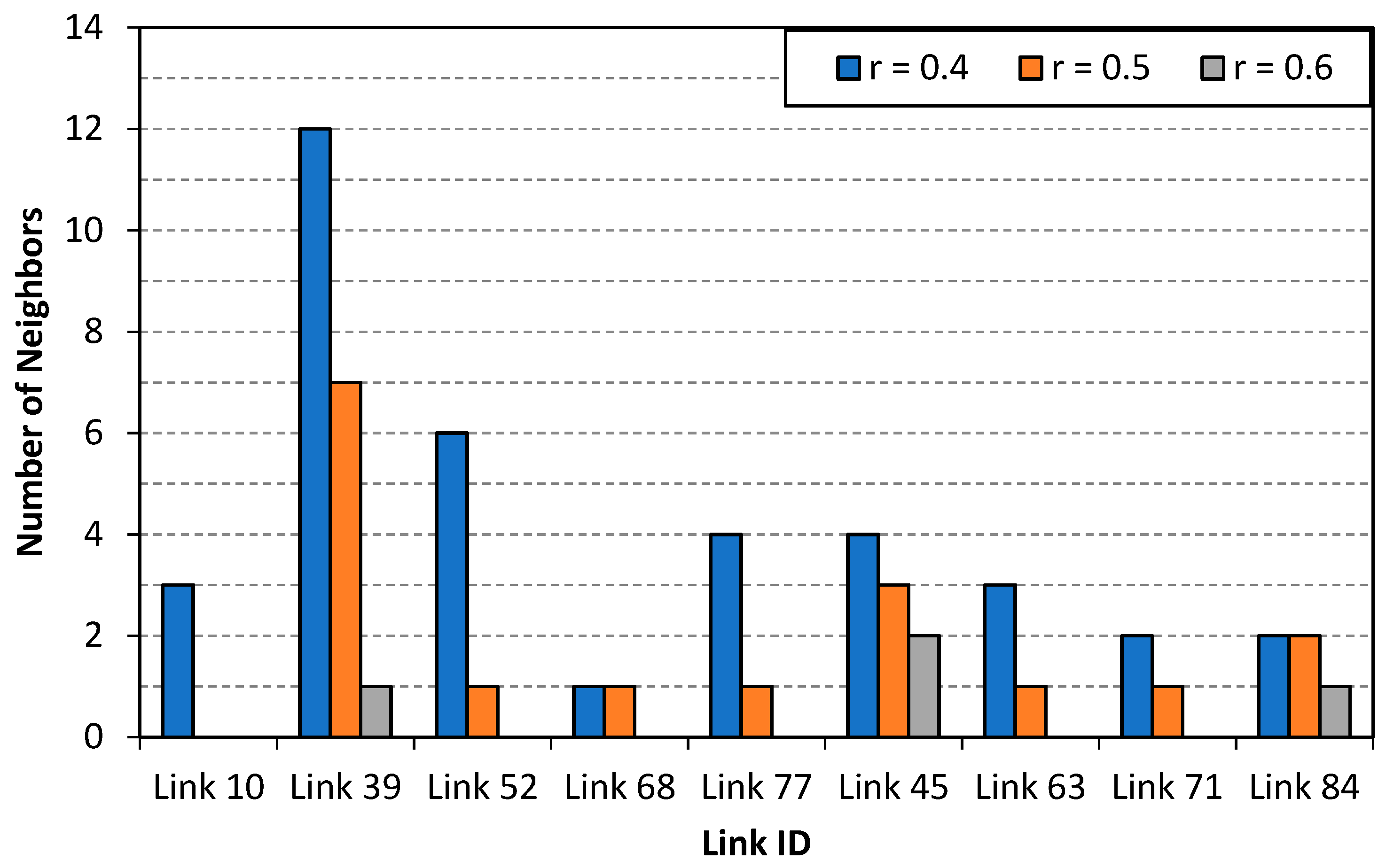
5.1. Link Neighbors Identification

In this study, link neighbors were identified using Pearson correlation. Travel time correlations were computed between the 100 links in Kuwait City network using the simulated travel time data. Only links with similar characteristics, located within the same area type, and have similar vehicle entry/exit movement directions were considered in the analysis. Therefore, travel time correlations only between 71 links were computed. Figure 4 presents the spatial travel time correlation between the links in the Kuwait City network. A correlation cut-off value of 0.4 was used to identify link neighbors. In total 592 link neighbors were identified for the 71 links with an average of 8 neighbors per link. Each link has at least one neighbor (except for 13 links, 18% of all links, were no neighbors were identified), with a maximum of 25 neighbors. In this study, nine links (link IDs 10, 39, 52, 68, 77, 45, 63, 71, 84) were randomly chosen from the network for the estimation of the travel times. Figure 5 shows the number of link neighbors identified for the nine links across different spatial correlation value.

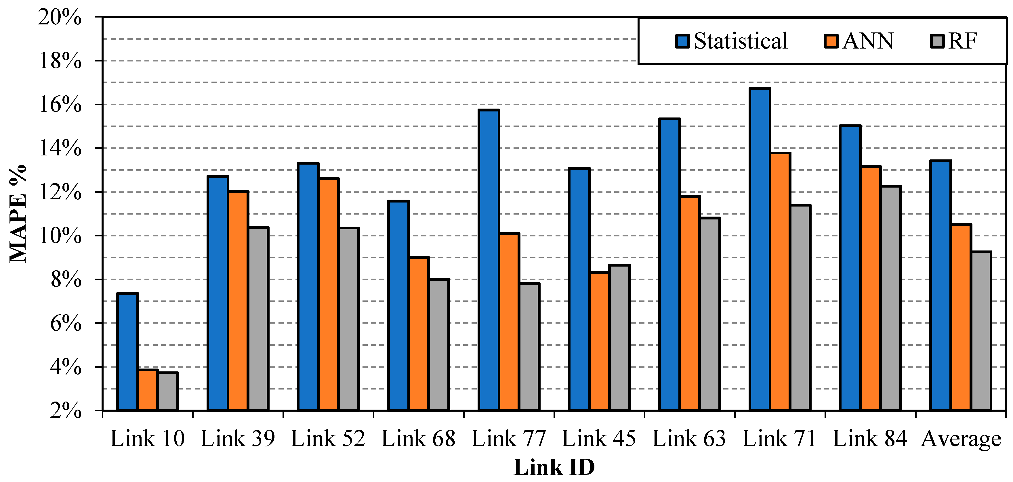
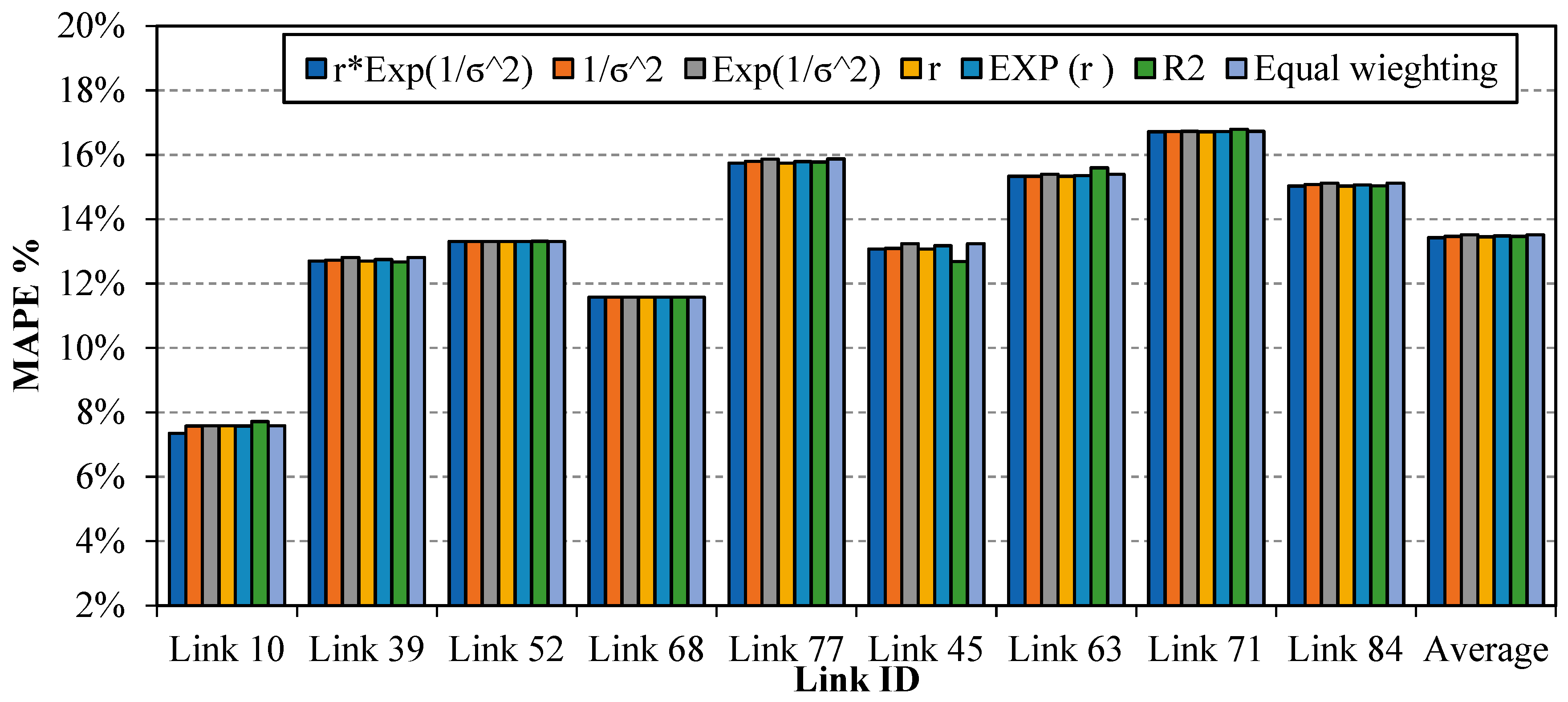
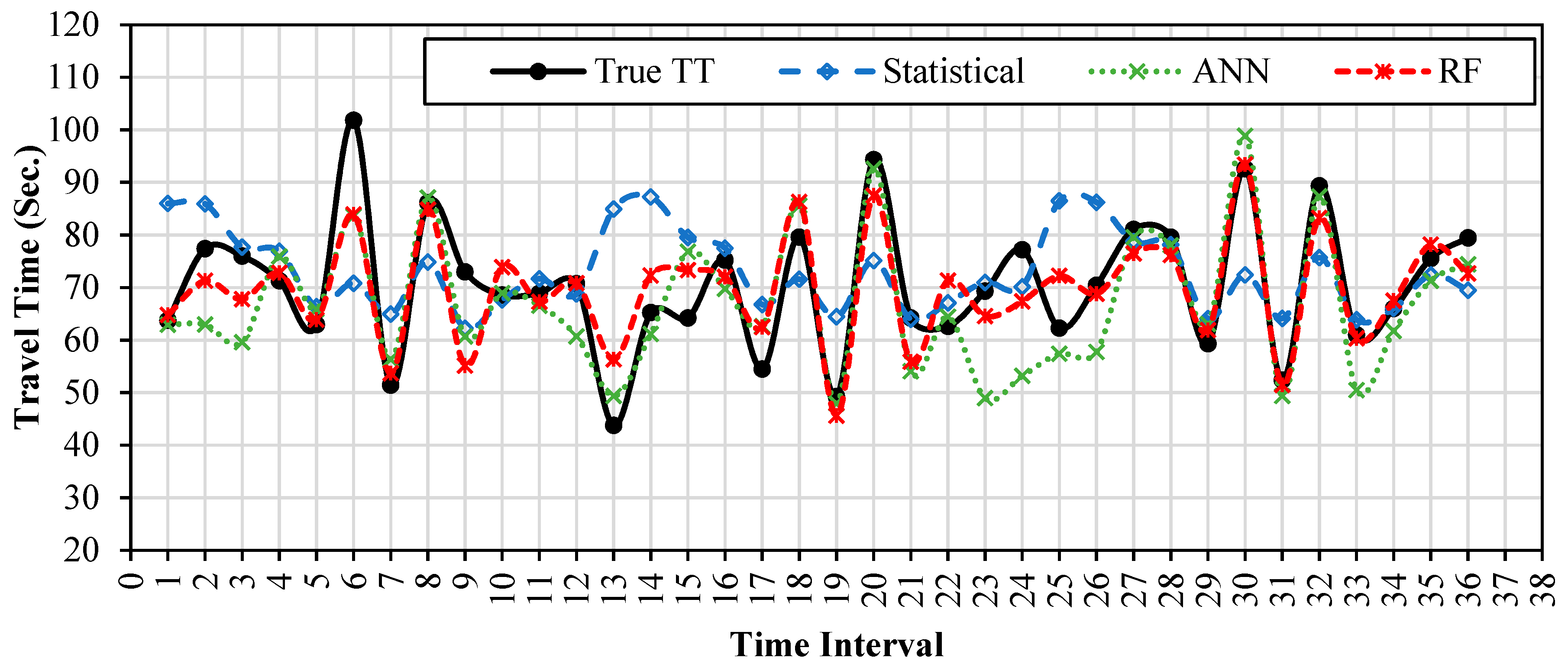
5.2. Travel Time Estimation Models

In this study, travel time estimation models were developed for the selected nine links—e.g., link ID 10, 39, 52, 68, 77, 45, 63, 71, and 84. The developed models relate link travel times with link neighbors. For the selected nine links, 37 link neighbors were identified at a correlation cut-off value of 0.4. Three different types of travel time estimation models—e.g., artificial neural network (ANN), random forest (RF), and statistical models—were developed. The models were developed using the training dataset, while the models’ performance was evaluated using the testing dataset.

For the statistical models, different regression models including the linear, power, exponential, and logarithmic that relate link travel times with each of its neighbor were developed. For the nine links considered in the analysis, 37 regression models were developed and only models with significant explanatory variables at p-value < 0.05 were considered. Linear regression models show a better fit than the power, exponential, and logarithmic models. The developed regression models were combined in a single mode for each link using the weighting schemes presented in Table 1. The weights $\mathsf{\alpha }$, and (1−$\mathsf{\alpha }$) for the real time estimation and the average historical travel time were estimated for each link during each period $t$. The best estimate for each link travel times during each interval $t$ was estimated. The performance of the statistical model is presented in Figure 6. Moreover, a sensitivity analysis was conducted to investigate the impact of the applied weighting schemes on the model performance, as shown in Figure 7. The results show that the accuracy of the statistical models is insensitive to the applied weighting schemes. As such, the combined weighting scheme of the correlation coefficient and models’ variances are used in the development of the statistical models later in the paper. The results show that the average estimation error for the nine links ranges between 7.6% and 16.7% with an average of 13.4%.

For the neural network model, multi-layer feed forward neural networks (MFFN) were developed for each link of the nine links considered in this study. The developed MFFN nets were trained using the training dataset. In the training process, the training dataset was split into two sets—e.g., training set and validation-training set which consist of around 85% and 15% of the training dataset, respectively. The validation-training dataset is used as stopping criteria for the training to avoid overfitting. The input parameters to the neural networks are link neighbors travel times, while the output parameters are the predicted link travel times. Three dense hidden layers were developed in each neural network with 30 neurons in both of the first and second hidden layers and 15 neurons in the third hidden layer. During the training process, a comparison of the prediction accuracy of the neural networks, while considering their complexity in terms of the number of hidden layers and neurons in each layer is performed. Different number of hidden layers (e.g., 1, 2, and 3 hidden layer(s)) and different number of neurons in each layers (e.g., 5, 10, 15, 20, 25, 30, 35, and 40 neurons) with a different transform function for each layer (e.g., logistic sigmoid and tangent sigmoid) is considered. The analysis shows that using three hidden layers with 30 neurons in the first two hidden layers and 15 neurons in the third hidden layer with a logistic sigmoid transform function in the first two hidden layers and a tangent sigmoid in the third hidden layer and the output layer provided the best prediction accuracy. Therefore, this structure was used to build the MFFN nets in this study, except for link ID 68 where the tangent sigmoid transfer function in all layers provided the best accuracy. The testing dataset (unseen data) were used in the performance evaluation of the MFFN net models. The performance of the MFFN nets is presented in Figure 6. The results show that the average estimation error of the MFFN model for the nine links ranges between 3.9% and 13.8% with an average of 10.5%, which outperforms the estimation performance of the statistical model. Significant estimation improvements were observed for links ID 10, 68, 77, 45, 63, 71, and 84 compared with the statistical models estimation.

Random forest (RF) models consisted of multiple decision trees were developed for each link of the nine links considered in this study. The models predict link travel times based on link neighbors real time travel times. The RF models were trained using the training dataset. In the training process, the training dataset was split into two sets, e.g., training set, and validation-training set which consist of around 85% and 15% of the training dataset, respectively. The validation-training dataset is used as stopping criteria for the training to avoid overfitting to determine the optimal number of variables at each tree split (m_try). During the training process, the bootstrap sampling is used to increase the variability between the decision trees in the forest. In the bootstrap sampling, each decision tree in the RF is trained using a different subsample of the training dataset. Moreover, a randomly selected subset of the input variables, e.g., link neighbors, was used to at each split of the tree (decision branching). Bootstrap sampling enables the computation of the error using the unused subset of the training dataset (out-of-bag OOB error). During the training process, a comparison of the prediction accuracy of the RF, while considering their complexity in terms of the number of variables to be considered in each decision tree split, is performed. A different number of variables at each decision tree split in each forest is considered starting from $m_{try}=1$ to $m_{try}=number of link neighbours-1$. A total number of 2000 trees is allowed to grow in each forest as the performance of the RF models is stable at 2000 trees. Similar results were reported in previous studies. Different 10 random seeds were considered in the analysis and the RF results presented in this paper is the average of the RF results from the different seeds. The analysis shows that using two variables $\left(m_{try}=2\right)$ at each decision tree split provided the best accuracy, except for links IDs 10, 68, 71, and 84 where using a single variable $\left(m_{try}=1\right)$ and for link ID 45 where using a number of variables of ($m_{try}=3$) at each decision tree split provided the best perdition accuracy. The final prediction of each RF model is the average of the prediction of each decision tree in the forest. The RF models’ performance was evaluated using the testing dataset. The performance of the RF models is presented in Figure 6.

The results show that the average estimation error of the RF model for the nine links ranges between 3.7% and 12.3% with an average of 9.3%. Both the RF and ANN models show improvements in estimation performance compared with the statistical model. For the nine links, the average improvement in the estimation accuracy when the RF is adopted ranges between 2.3% and 7.9% with an average of 4.2% compared with the statistical model. The performance of the RF was slightly better compared with the ANN model. The average improvement in the estimation accuracy when the RF model is adopted is 1.3% with a maximum improvement of 2.4% compared with the ANN model. An example of travel time model estimation for link ID 77 is presented in Figure 8.

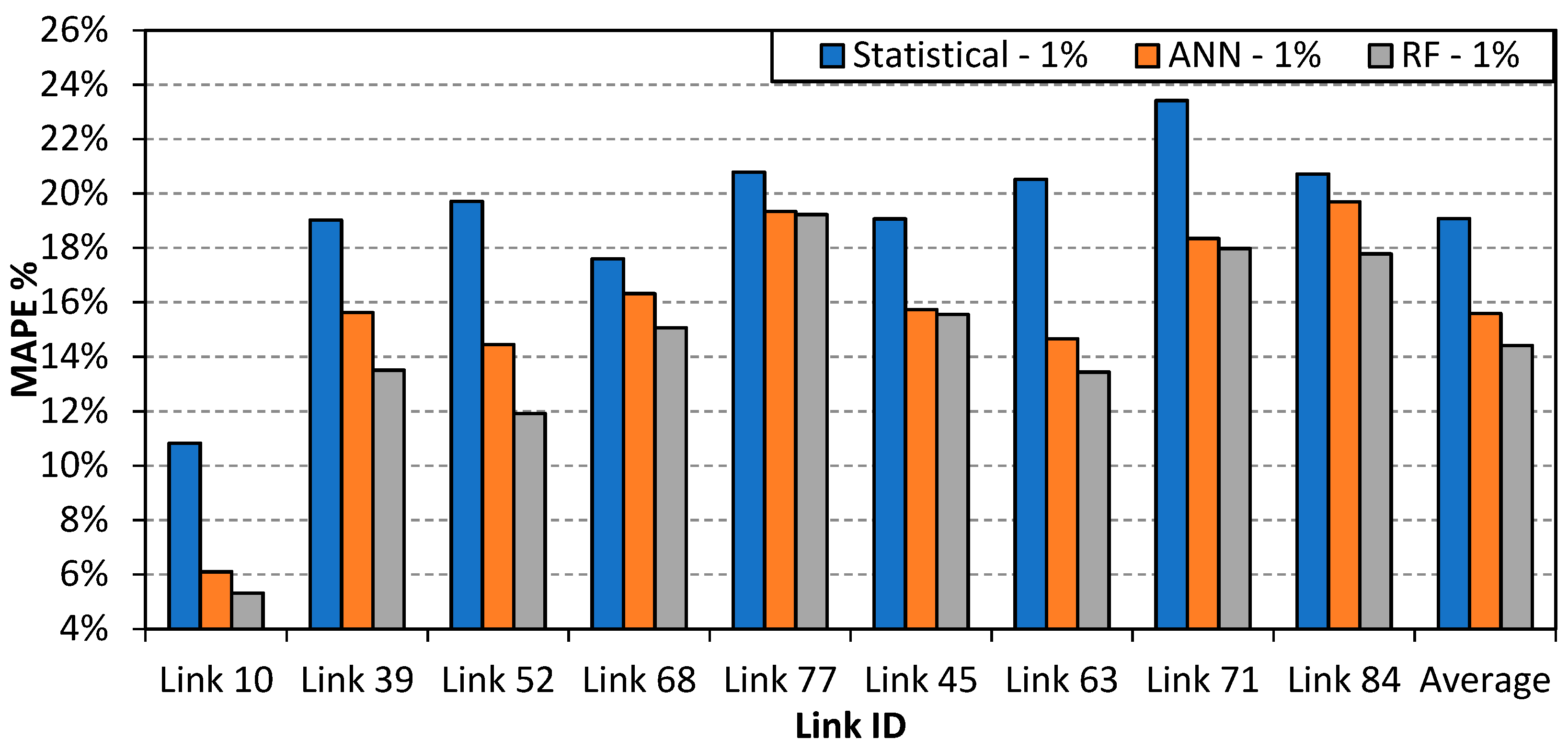
5.3. Model Performance in Partial Network Coverage

In a practical implementation of the travel time estimation system, probe vehicles—e.g., taxi fleet—can be used for collecting network link real time data. In such a case, there is a possibility that no probe vehicles passes through one or all of the link neighbors during each time period $t$ (i.e., no real time travel time available on one or more of link neighbor). In such a case where no real time data is available on all link neighbors, link historical travel time can be used. Nevertheless, in cases where some of the link neighbors are covered by probe vehicles, the travel time estimation models—e.g., ANN, RF, and statistical models—can be used to estimate the link real time travel time using the available real time travel time on link neighbors at each time period $t$. To investigate this issue, three probe market penetration rates of 1%, 3%, and 5% were considered in the analysis. Similar to the previous analysis, simulated travel times were generated for different 10 traffic demand scenario of the pm peak period. The simulated data were generated for traffic demand levels of 60% to 105% with an increment of 5%. A travel time period of 5-min is considered in the analysis, e.g., each hour of the demand level consists of 12 analysis periods. The simulated data was split into two sets; the training data set which form 70% of the data, and the testing data set which form 30% of the data. For the training dataset, average link travel times were computed using all the vehicles passes the link during the time period $t$. For the testing dataset, the true link travel times were computed as the mean of the travel time of all vehicles passing the target link during the time period $t$. While the link neighbor travel times were computed as the mean travel times of probe vehicles passing link neighbors during the time period $t$.

Random forest (RF) models and multi-layer feed forward neural networks (MFFN) were developed for the nine links considered in the analysis based on the available link neighbors during each time period $t$. For the statistical models, the weighting scheme assigns a value of zero for the link neighbors not covered by probe vehicles during the time period $t$—i.e., the estimation is only based on the available link neighbors on each time period $t$. The performance of the three models at different probe penetration rates are presented in Figure 9, Figure 10 and Figure 11. The performance of the models was evaluated using the testing dataset. The results show that the RF and ANN models significantly outperform the statistical model, especially at a low probe penetration rate of 1%. The RF and the ANN models have a higher average estimation accuracy of about 4.7% and 3.5% compared with the statistical model at a probe penetration rate of 1%, respectively. At a probe penetration rate of 1%, the RF, MFFN, and the statistical models correctly estimate real time travel times with estimation accuracies of 85.6%, 84.4%, and 80.9% respectively. Moreover, the results show that the accuracy of the models increase as the probes’ penetration rates increase from 1% to 3%. However, beyond 3%, no significant increase in the estimation accuracy is observed compared to the penetration rate of 5%.

Furthermore, link coverage was evaluated at the three probe penetration rates. Link coverage was computed as the percentage of the number of intervals at which the real time travel times are available, for at least one link neighbor, during the total measurement periods. Figure 12 shows the average coverage of the link neighbors at the different probe penetration rates. The results show that the average coverage of the links reaches 73.8% at a probe penetration rate of 1%. However, the coverage of links significantly increases as the probe penetration rate increases to 3% and 5%. The average link coverage reaches about 94.8% and 97.2% at probes penetration rates of 3% and 5%, respectively.

6. Discussion and Conclusions

This article focuses on link travel time estimation in partial network coverage using the data obtained from probe vehicles. Travel time is an important metric for network performance and is vital in helping road users in better shouldering their trips. Few studies discussed the application of random forest (RF) and multi-layer feed forward neural network (MFFN) in estimating and predicting travel times in urban networks that are partially covered by moving sensors. Therefore, this study proposes two machine learning approaches—e.g., RF and MFFN—to estimate real time travel times in urban networks that are partially covered by moving sensors. The RF approach is an ensemble learning algorithm that is based on a voting/averaging mechanism in the prediction of the travel times. The neural network, which is an artificial intelligence approach, was trained using the back-propagation learning algorithm, and the neural weights were updated using the Levenberg–Marquardt optimization technique. The performance of these methods was compared to statistical travel time estimation model that uses the empirical Bayes (EB) method. The performance of the models was analyzed at different traffic demand scenarios. The results show that the proposed RF and MFFN models provided better estimation accuracy compared with the statistical model, however the difference was not significantly considerable. As well, the performance of the RF was marginally better than the MFFN. In terms of the computation cost, the RF model is more efficient and required less CPU computation time compared with multi-layer feed forward neural network (MFFN). Furthermore, the study investigated the impact of the probe penetration rate on real time neighbor links coverage. Results show that at probe penetration rates of 1%, 3%, and 5%, the models cover the estimation of the real time travel times on 73.8%, 94.8%, and 97.2% of the estimation intervals.

Recently, the use of traffic intelligent [33,34] and machine learning techniques [35] in various transportation studies is spreading for their potential in providing accurate results. Investigating the performance of other methods—e.g., gradient boosting and AdaBoost—in estimating and predicting travel times in urban network that are partially covered moving sensors can be considered in future research. Conducting extensive validation of the proposed methods using a large-scale real-world data should be considered. As well, investigating the impact of using historical travel times with the real time travel times on the estimation accuracy of the machine learning techniques can be investigated in future research. Considering other approaches in identifying link neighbors can also be investigated. Other approaches involve identifying link neighbors based on the variable importance obtained from the RF model. Investigating the impact of the used learning algorithm and the designing structure of the neural network on the performance of the neural nets can also be considered in future research. Future work can focus on analyzing the computational cost associated with continuous training of each method, especially when applied throughout a large transport network, as the travel time is an aspect that depends on multiple factors, some of which are very dynamic.

References

1. Li, L.; Chen, X.; Li, Z.; Zhang, L. Freeway Travel-Time Estimation Based on Temporal–Spatial Queueing Model. IEEE Trans. Intell. Transp. Syst. 2013, 14, 1536–1541. [Google Scholar] [CrossRef]
2. Coifman, B. Estimating travel times and vehicle trajectories on freeways using dual loop detectors. Transp. Res. Part A Policy Pr. 2002, 36, 351–364. [Google Scholar] [CrossRef]
3. Zheng, F.; Van Zuylen, H. Urban link travel time estimation based on sparse probe vehicle data. Transp. Res. Part C Emerg. Technol. 2013, 31, 145–157. [Google Scholar] [CrossRef]
4. Rahmani, M.; Koutsopoulos, H.N.; Jenelius, E. Travel time estimation from sparse floating car data with consistent path inference: A fixed point approach. Transp. Res. Part C Emerg. Technol. 2017, 85, 628–643. [Google Scholar] [CrossRef]
5. Tang, K.; Chen, S.; Liu, Z.; Khattak, A.J. A tensor-based Bayesian probabilistic model for citywide personalized travel time estimation. Transp. Res. Part C Emerg. Technol. 2018, 90, 260–280. [Google Scholar] [CrossRef]
6. Sanaullah, I.; Quddus, M.; Enoch, M. Developing Travel Time Estimation Methods Using Sparse GPS Data. J. Intell. Transp. Syst. 2016, 20, 532–544. [Google Scholar] [CrossRef]
7. Rilett, L.R.; Park, D. Direct Forecasting of Freeway Corridor Travel Times Using Spectral Basis Neural Networks. Transp. Res. Rec. J. Transp. Res. Board 2001, 1752, 140–147. [Google Scholar] [CrossRef]
8. Chen, B.Y.; Lam, W.H.; Sumalee, A.; Li, Z.-L. Reliable shortest path finding in stochastic networks with spatial correlated link travel times. Int. J. Geogr. Inf. Sci. 2012, 26, 365–386. [Google Scholar] [CrossRef]
9. Chan, K.S.; Lam, W.H.K.; Tam, M.L. Real time Estimation of Arterial Travel Times with Spatial Travel Time Covariance Relationships. Transp. Res. Rec. J. Transp. Res. Board 2009, 2121, 102–109. [Google Scholar] [CrossRef]
10. El Esawey, M.; Sayed, T. Travel time estimation in urban networks using limited probes data. Can. J. Civ. Eng. 2011, 38, 305–318. [Google Scholar] [CrossRef]
11. Alrukaibi, F.; Alsaleh, R.; Sayed, T. Real time travel time estimation in partial network coverage: A case study in Kuwait City. Adv. Transp. Stud. 2018, 44, 79–94. [Google Scholar]
12. Jenelius, E.; Koutsopoulos, H.N. Travel time estimation for urban road networks using low frequency probe vehicle data. Transp. Res. Part B Methodol. 2013, 53, 64–81. [Google Scholar] [CrossRef] [Green Version]
13. Liu, H.X.; Ma, W. A virtual vehicle probe model for time-dependent travel time estimation on signalized arterials. Transp. Res. Part C Emerg. Technol. 2009, 17, 11–26. [Google Scholar] [CrossRef]
14. Jula, H.; Dessouky, M.; Ioannou, P.A. Real time Estimation of Travel Times along the Arcs and Arrival Times at the Nodes of Dynamic Stochastic Networks. IEEE Trans. Intell. Transp. Syst. 2008, 9, 97–110. [Google Scholar] [CrossRef]
15. Zhang, Z.; Wang, Y.; Chen, P.; He, Z.; Yu, G. Probe data-driven travel time forecasting for urban expressways by matching similar spatiotemporal traffic patterns. Transp. Res. Part C Emerg. Technol. 2017, 85, 476–493. [Google Scholar] [CrossRef]
16. Gajewski, B.J.; Rilett, L.R. Estimating link travel time correlation: An application of Bayesian smoothing splines. J. Transp. Stat. 2005, 7, 53–70. [Google Scholar]
17. Zeng, W.; Miwa, T.; Wakita, Y.; Morikawa, T. Application of Lagrangian relaxation approach to α -reliable path finding in stochastic networks with correlated link travel times. Transp. Res. Part C Emerg. Technol. 2015, 56, 309–334. [Google Scholar] [CrossRef]
18. Seo, T.; Kusakabe, T. Probe vehicle-based traffic state estimation method with spacing information and conservation law. Transp. Res. Part C Emerg. Technol. 2015, 59, 391–403. [Google Scholar] [CrossRef] [Green Version]
19. Hellinga, B.; Fu, L. Assessing Expected Accuracy of Probe Vehicle Travel Time Reports. J. Transp. Eng. 1999, 125, 524–530. [Google Scholar] [CrossRef] [Green Version]
20. El Esawey, M.; Sayed, T. A framework for neighbour links travel time estimation in an urban network. Transp. Plan. Technol. 2012, 35, 281–301. [Google Scholar] [CrossRef]
21. Muknahallipatna, S.; Chowdhury, B.H. Input Dimension Reduction in Neural Network Training-Case Study in Transient Stability Assessment of Large Systems. In Proceedings of the International Conference on Intelligent System Application to Power Systems, Orlando, FL, USA, 28 January–2 February 1996. [Google Scholar]
22. Breiman, L. Random forests. Mach. Learn. 2001, 45, 5–32. [Google Scholar] [CrossRef]
23. Hastie, T.; Tibshirani, R.; Friedman, J.; Franklin, J. The Elements of Statistical Learning: Data Mining, Inference, and Prediction, 12th ed.; Springer Series in Statistics: New York, NY, USA, 2017. [Google Scholar]
24. Biau, G. Analysis of a random forests model. J. Mach. Learn. Res. 2012, 13, 1063–1095. [Google Scholar]
25. Oshiro, T.M.; Perez, P.S.; Baranauskas, J.A. How Many Trees in a Random Forest? In Machine Learning and Data Mining in Pattern Recognition; Springer: Berlin/Heidelberg, Germany, 2012. [Google Scholar]
26. Laña, I.; Lobo, J.L.; Capecci, E.; Del Ser, J.; Kasabov, N. Adaptive long-term traffic state estimation with evolving spiking neural networks. Transp. Res. Part C Emerg. Technol. 2019, 101, 126–144. [Google Scholar] [CrossRef]
27. Torlai, G.; Mazzola, G.; Carrasquilla, J.; Troyer, M.; Melko, R.; Carleo, G. Neural-network quantum state tomography. Nat. Phys. 2018, 14, 447–450. [Google Scholar] [CrossRef] [Green Version]
28. Fausett, L. Fundamentals of Neural Networks: Architectures, Algorithms, and Applications; Englewood Cliffs: Prentice-Hall, NJ, USA, 1994. [Google Scholar]
29. Levenherg, K. A method for the solution of certain problems in least squares. Quart. Appl. Math. 1994, 2, 164–168. [Google Scholar] [CrossRef]
30. Marquardt, D.W. An Algorithm for Least-Squares Estimation of Nonlinear Parameters. J. Soc. Ind. Appl. Math. 1963, 11, 431–441. [Google Scholar] [CrossRef]
31. El Esawey, M.; Sayed, T. Using buses as probes for neighbor links travel time estimation in an urban network. Transp. Lett. 2011, 3, 279–292. [Google Scholar] [CrossRef]
32. Sen, A.; Thakuriah, P.; Zhu, X.Q.; Karr, A. Frequency of probe reports and variance of travel time estimates. J. Transp. Eng. 1997, 123, 290–297. [Google Scholar] [CrossRef]
33. Alsaleh, R.; Sayed, T.; Zaki, M.H. Assessing the Effect of Pedestrians’ Use of Cell Phones on Their Walking Behavior: A Study Based on Automated Video Analysis. Transp. Res. Rec. J. Transp. Res. Board. 2018, 2672, 46–57. [Google Scholar] [CrossRef]
34. Alsaleh, R.; Hussein, M.; Sayed, T. Microscopic Behavioural Analysis of Cyclists and Pedestrians Interactions in Shared Space. Can. J. Civ. Eng. 2019. In press. [Google Scholar] [CrossRef]
35. Abduljabbar, R.; Dia, H.; Liyanage, S.; Bagloee, S. Applications of artificial intelligence in transport: An overview. Sustainability 2019, 11, 189. [Google Scholar] [CrossRef]
Figure 1. Random forest process.
Sustainability 11 03822 g001
Figure 2. Multi-layer feed forward neural network (MFFN) model.
Sustainability 11 03822 g002
Figure 3. Urban road network of Kuwait City [11].
Sustainability 11 03822 g003
Figure 4. Spatial travel time correlation between the links.
Sustainability 11 03822 g004
Figure 5. Number of link neighbors at different correlation cut-off values.
Sustainability 11 03822 g005
Figure 6. Model performance.
Sustainability 11 03822 g006
Figure 7. Statistical model performance using different weighting schemes.
Sustainability 11 03822 g007
Figure 8. Travel time model estimation for link 77 during different time intervals.
Sustainability 11 03822 g008
Figure 9. Model performance at 1% probe rate.
Sustainability 11 03822 g009
Figure 10. Model performance at 3% probe rate.
Sustainability 11 03822 g010
Figure 11. Model performance at 5% probe rate.
Sustainability 11 03822 g011
Figure 12. Link coverage at different probe penetration rates.
Sustainability 11 03822 g012