Depicting Flows of Embodied Water Pollutant Discharge within Production System: Case of an Undeveloped Region

Abstract

Water pollution is still an obstacle on the way towards sustainable development, especially for some undeveloped regions in China. To formulate policies for water pollution control from multiple perspectives, it is significant to holistically investigate how final demand purchases trigger water pollutant discharge in the production process. With Jilin Province as an empirical study area, the final production and consumption attributions of chemical oxygen demand (COD) discharge within the input–output framework are measured. By employing structural pass analysis and mapping approaches, the supply chain linkages between the two attributions of COD discharge are illustrated. The embodied flows of COD discharge across sectors through the supply chains are exhaustively revealed. The results show that the exports drive 70.23% of the total COD discharge. Animal production (S2) is the dominant contributor to COD discharge from both production and consumption perspectives. Final demand on the products of Foods & tobacco products (S8), Sawmills & furniture, and Construction largely induces COD discharge at higher production layers. In contrast, final demand on S2’s products mainly drives direct COD discharge (96.04%). S2 and S8 are the two key sectors in the supply chains, which provide other sectors with pollution-intensive products as intermediate inputs. The findings indicate that the export of S2’s products should be largely cut down, along with adjustment of the export structure. Innovations of production technologies and improvement of end-of-pipe abatement abilities for S2 and S8 should be facilitated. Besides, cutting capacity or reducing investment on these two sectors should be propelled.

1. Introduction

As a critical case for negative externalities of the economy, water pollution has triggered the deterioration of water eco-environment, shrinkage of utilizable volume of water resources and threats to human health, especially in the developing countries or regions [1,2]. China, a middle-income country, is still confronted with the challenges of water pollution in spite that some policies and measures for water pollution control have been implemented [3,4]. Meanwhile, rapid economic development is aggravating the difficulty in coping with water pollution issues. Control of water pollutant discharge and promotion of structural transformation of the economy were therefore jointly proposed for the first time in China’s “Action Plan for Prevention and Control of Water Pollution” in 2015. Clarification of the relationships between water pollutant discharge and economic activities is indispensable for proposing efficient policies and measures to accomplish pollutant discharge reduction and meanwhile promote sustainable development [5]. Considering that the water pollutants discharged in the production process can ultimately be attributed to final demand purchases, both the production-based and consumption-based discharge inventories should be investigated. Subsequently, the embodied water pollutants in the flows of intermediate products (goods and services) along the supply chains also need to be quantified to illustrate how water pollutant discharge “flows” from producers to consumers and investors in capital [6].

Environmentally extended input–output (EEIO) analysis has been applied to describe and investigate the economic and environmental linkages among industrial sectors [7,8,9,10,11,12], since Leontief’s pioneering research work [13]. As final demand instigates emissions in the production process [9], consumption-based accounting of pollutants and carbon dioxide (CO₂) emissions was therefore performed to uncover the final attributions of the embodied emissions (including direct and indirect emissions) using the EEIO models [14,15,16,17]. Such an approach helps to identify the responsibilities for emissions from the view of final consumers. Simultaneously, EEIO models were also used to conduct comparative analysis between production-based and consumption-based emissions [18,19,20,21,22], which was essential for formulating policies and measures form producer and consumer perspectives. However, determination of the attributions of water pollutant discharge among production sectors or final demand categories was rarely carried out within an EEIO framework.

The disparities between production and consumption attributions of emissions revealed by the above contributions can be further investigated by capturing the flows of emissions embodied in products [6]. Structure path analysis (SPA) based on an input–output (IO) framework is capable of excavating the intricate supply chain of production process [17,23]. Thus, SPA can be used to explore the transmission of embodied emissions across different sectors at different layers and identify the key sectors and paths with high environmental impacts [24,25,26,27], which may help to perform more sound environmental policies [24]. SPA has been successfully applied to capture and analyze the flows of energy [28,29,30], natural resources (such as minerals) [31,32], embodied emissions of CO₂ [9,25,33,34,35,36] and air pollutants [17,37,38,39], and water resources [40,41], across the IO supply chains. However, most of the empirical studies made efforts on energy use and related emissions. To the best of our knowledge, studies focusing on water pollutant discharge based on SPA have not been undertaken.

Theoretically, infinite supply chains through a production system can be triggered by final demand within an IO framework. It is impossible to actually obtain all the supply chains using SPA method. While, the emissions embodied in the summation of less important supply chains account for a considerable share of the total [42]. Thus, Skelton et al. initially proposed a “methodological and diagrammatic approach” based on SPA to depict the flows of embodied emissions through the economy [6]. This novel mapping approach measured the emission flow in each relatively important supply chain, meanwhile, solved the infinite issue by calculating the total emissions embodied in the less important supply chains with more layers in the upstream of the production system. The merits of this approach are that both quantitative and diagrammatic information for the flows of embodied emissions can be provided, and the connections among the attributions of final production, intermediate consumption and final consumption can be exhaustively illustrated.

Water pollution is still one of the toughest environmental challenges for some regions or basins, however, few efforts have been made to quantify the demand-driven water pollutant discharge and depict water pollutant transmissions through the production system. To fill these gaps, this paper conducts an empirical study with Jilin Province, an undeveloped region of China characterized with heavy water pollution (Chemical oxygen demand, COD, is selected as the water pollutant indicator considering its leading contribution to water pollution) as the study area. Even though some measures focusing on end-of-pipe control have been implemented, the water environmental quality of the study area has not been improved observably. Terribly, the water environmental quality of some regions keeps deteriorating alongside economic development [5]. The pessimistic status is due to the lack of the proposal of policies and measures from view of an integrated system of the water environment and social economy. Thus, it calls for a systematic analysis for presenting the flows of water pollutants within the production system, identification of how final demand drives water pollutant discharge and provision of feasible policy recommendations of water pollution control from a systematic perspective for the study area.

This study intends to clarify the final production and consumption attributions of domestic COD discharge based on the 2012 regional IO table (latest released). For the first time, SPA and the above mapping approach are collectively applied to illustrate how the embodied COD discharge flows from producers to consumers, and extract the key sectors and paths of the embodied COD discharge driven by final demand. Additionally, a sector’s total consumption attribution of COD discharge (COD discharge embodied in all intermediate and final products of a sector) is measured based on the Pure Backward Linkage Measure [43], to calculate the contributions of final production and consumption attributions of COD discharge to a sector’s overall impact. The results may help to facilitate the identification of the responsibilities of the economic actors on COD discharge and to formulate policies for supply chain management in view of COD discharge control.

2. Methodology and Data

2.1. Non-Competitive Environmentally Extended Input–Output Model

Based on the fundamental formula of Leontief model, the regional IO monetary flows among sectors are expressed as:

$$\mathit{X}={\left(\mathit{I}-\mathit{A}\right)}^{-1}\left(\mathit{C}+\mathit{K}+\mathit{E}-\mathit{M}\right)$$

(1)

where X is the vector of total output; I is the identity matrix; A is the input coefficient matrix; $\mathit{L}={\left(\mathit{I}-\mathit{A}\right)}^{-1}$ denotes the Leontief inverse matrix; C is the consumption vector; K is the vector of capital formation; E and M are the vectors of exports and imports, respectively.

In this study, only the domestic inputs are involved to estimate the local COD discharge. Thus, the imports should be removed from the intermediate inputs and final demand. The critical assumption used for eliminating imports is that each final demand category and each sector use the imports with the same proportions referring to Weber et al. [44], Zhao et al. [45] and Guan et al. [46]. The input coefficient matrix of a completive IO model can be further decomposed as:

$$\mathit{A}={\mathit{A}}^m+{\mathit{A}}^d$$

(2)

$${\mathit{A}}^d=\left(\mathit{I}-\hat{\mathit{R}}\right)\mathit{A}$$

(3)

where A^m and A^d represent the coefficient matrices that estimate the imported and domestic inputs, respectively; $\hat{\mathit{R}}$ reflects the diagonal matrix of vector $\mathit{R}=\left[r_i\right]=\left[{\mathit{m}}_{\mathit{i}}/\left({\mathit{m}}_{\mathit{i}}+{\mathit{x}}_{\mathit{i}}\right)\right]$ that denotes the import portion of the input coefficients (m_i and x_i are the elements of M and X, respectively).

Therefore, a new balance considering only domestic inputs and final demand on domestically-produced products (Y^d) is derived as:

$$\mathit{X}={\left(\mathit{I}-{\mathit{A}}^d\right)}^{-1}{\mathit{Y}}^d={\mathit{L}}^d\left({\mathit{F}}^d+{\mathit{E}}^d\right)={\mathit{L}}^d\left({\mathit{C}}^d+{\mathit{K}}^d+{\mathit{E}}^d\right)$$

(4)

where ${\mathit{L}}^d={\left(\mathit{I}-{\mathit{A}}^d\right)}^{-1}$ denotes the domestic Leontief inverse matrix; F^d is the vector of domestic final demand on domestically-produced products; C^d, K^d and E^d are the vectors of consumption, capital formation and exports of domestically-produced products.

Subsequently, the production-based and consumption-based accountings of local COD discharge are determined as follows:

$${\mathit{P}}^{final}=\hat{\mathit{w}}{\mathit{L}}^d{\mathit{Y}}^d$$

(5)

$${\mathit{Q}}^{final}=\mathit{w}{\mathit{L}}^d{\hat{\mathit{Y}}}^d$$

(6)

where ${\mathit{P}}^{final}$ is the column vector of final production attributions of COD discharge; ${\mathit{Q}}^{final}$ is the row vector of final consumption attributions of COD discharge; $\hat{\mathit{w}}$ denotes the diagonal matrix of w which is the row vector of COD discharge intensity.

2.2. Structural Path Analysis

To conduct a SPA for the domestic supply chain of COD discharge, the domestic Leontief inverse matrix L^d discussed in Section 2.1 is expanded using the power series approximation as [17,29]:

$${\mathit{L}}^d={\left(\mathit{I}-{\mathit{A}}^d\right)}^{-1}=\mathit{I}+{\mathit{A}}^d+{\left({\mathit{A}}^d\right)}^2+{\left({\mathit{A}}^d\right)}^3+\dots {\left({\mathit{A}}^d\right)}^t$$

(7)

A production layer (PL) is defined as each stage in the expansion in Equation (7), PL^t = A^t. Then, the relationship between the adjacent two layers is that the production of intermediate products in the (t + 1)-th layer is used as the inputs into the t-th layer, PL^t+1 = PL^tA^t. The COD discharge embodied in final demand on domestically-produced products can be therefore expanded as:

$$\mathit{w}{\mathit{L}}^d{\mathit{Y}}^d=\mathit{w}\mathit{I}{\mathit{Y}}^d+\mathit{w}{\mathit{A}}^d{\mathit{Y}}^d+\mathit{w}{\left({\mathit{A}}^d\right)}^2{\mathit{Y}}^d+\mathit{w}{\left({\mathit{A}}^d\right)}^3{\mathit{Y}}^d+\dots \mathit{w}{\left({\mathit{A}}^d\right)}^t{\mathit{Y}}^d$$

(8)

where $\mathit{w}{\left({\mathit{A}}^d\right)}^t{\mathit{Y}}^d$ denotes the contribution of the t-th production layer to the embodied COD discharge.

In SPA, it is clear that $\mathit{w}{\left({\mathit{A}}^d\right)}^t{\mathit{Y}}^d$ in Equation (8) is used to measure the direct COD discharge at the t-th layer of the supply chain. For instance, three SPA equations used to illustrate the direct COD discharge driven by final demand at PL¹, PL² and PL³ are expressed as $D_{\mathit{ji}}^{1\to 0}=w_j{A}_{\mathit{ji}}^d{Y}_i^d$, $D_{\mathit{uji}}^{2\to 0}=w_u{A}_{\mathit{uj}}^d{A}_{\mathit{ji}}^d{Y}_i^d$, $D_{\mathit{luji}}^{3\to 0}=w_l{A}_{\mathit{lu}}^d{A}_{\mathit{uj}}^d{A}_{\mathit{ji}}^d{Y}_i^d$, respectively (D is the symbol of direct discharge). In practice, it is impossible to capture the infinite paths, while SPA makes it possible to trace the important paths for pollutant discharge that starts from a final demand purchase and ends up with a polluting production sector. Moreover, the distribution of direct pollutant discharge instigated by final demand in all production layers through the supply chain can be depicted for each sector using SPA.

2.3. Depicting Flows of Embodied Discharge

For uncovering how and why the differences between final production and consumption attributions of pollutant discharge occur, a quantitative and diagrammatic mapping approach is applied. The intermediate consumption attributions of pollutant discharge are measured. The embodied flows of pollutant discharge which connect final production, intermediate consumption and final consumption attributions of pollutant discharge are illustrated. A key pollutant discharge multiplier matrix S is calculated as:

$$\mathit{S}=\hat{\mathit{w}}{\mathit{L}}^d$$

(9)

Then, a new multiplier s is derived as the column sum of S. An element s_j of multiplier s is used to calculate pollutant discharge from all production sectors that have become embodied in sector j’s unit output. Both direct and indirect pollutant discharge are involved in multiplier s, which helps to determinate the final and intermediate consumption attributions of COD discharge by post-multiplying final and intermediate demand, respectively (see

Table 1. Attribution equations of pollutant discharge for PL⁰ to PL^3.

	Final Attributions (PL0)	Intermediate Attributions at PL1	Intermediate Attributions at PL2	Intermediate Attributions at PL3
Direct	$D_{{}_i}^0=w_i{Y}_i^d$	$D_j^1=w_j{\mathit{A}}_{j:}^d{\mathit{Y}}^d$	$D_u^2=w_u{\mathit{A}}_{u:}^d{\mathit{A}}^d{\mathit{Y}}^d$	$D_l^3=w_l{\mathit{A}}_{l:}^d{\mathit{A}}^d{\mathit{A}}^d{\mathit{Y}}^d$
Consumption	$Q_{{}_i}^0=s_i{Y}_i^d$	$Q_j^1=s_j{\mathit{A}}_{j:}^d{\mathit{Y}}^d$	$Q_u^2=s_u{\mathit{A}}_{u:}^d{\mathit{A}}^d{\mathit{Y}}^d$	$Q_l^3=s_l{\mathit{A}}_{l:}^d{\mathit{A}}^d{\mathit{A}}^d{\mathit{Y}}^d$
Production	$P_i^0={\mathit{S}}_{i:}{\mathit{Y}}^d$	$P_j^1={\mathit{S}}_{j:}{\mathit{A}}^d{\mathit{Y}}^d$	$P_u^2={\mathit{S}}_{u:}{\mathit{A}}^d{\mathit{A}}^d{\mathit{Y}}^d$	$P_l^3={\mathit{S}}_{l:}{\mathit{A}}^d{\mathit{A}}^d{\mathit{A}}^d{\mathit{Y}}^d$

Subscripts i, j, u, l, and “:” represent the sector at PL⁰, PL¹, PL², PL³, and all sectors, respectively.

). Another multiplier S_i: (subscript “:” denotes all sectors) obtained from multiplier S estimates pollutant discharge from sector i that have become embodied in all sectors’ unit output. Post-multiplication of multiplier S_i: by final and intermediate demand measures sector i’s final and intermediate production attributions of COD discharge, respectively (Table 1). More detailed information (with examples) for the above multipliers can be referred to the contribution of Skelton et al. [6].

The calculation of attributions of pollutant discharge at different layers has been expressed in Table 1. The embodied flows of pollutant discharge among different layers across sectors need to be measured. The set of equations for calculating the embodied flows of pollutant discharge is presented in

Table 2. Equations of embodied pollutant discharge flows among layers in the production system.

	to Sector i at PL0	to Sector j at PL1	to Sector u at PL2
from sector j at PL1	$Q_{\mathit{ji}}^{1\to 0}=s_j{A}_{\mathit{ji}}^d{Y}_i^d$
from sector u at PL2	$Q_{\mathit{uji}}^{2\to 0}=s_u{A}_{\mathit{uj}}^d{A}_{\mathit{ji}}^d{Y}_i^d$	$Q_{\mathit{uj}}^{2\to 1}=s_u{A}_{\mathit{uj}}^d{\mathit{A}}_{j:}^d{\mathit{Y}}^d$
from sector l at PL3	$Q_{\mathit{luji}}^{3\to 0}=s_l{A}_{\mathit{lu}}^d{A}_{\mathit{uj}}^d{A}_{\mathit{ji}}^d{Y}_i^d$	$Q_{\mathit{luj}}^{3\to 1}=s_l{A}_{\mathit{lu}}^d{A}_{\mathit{uj}}^d{\mathit{A}}_{j:}^d{\mathit{Y}}^d$	$Q_{\mathit{lu}}^{3\to 2}=s_l{A}_{\mathit{lu}}^d{\mathit{A}}_{u:}^d{\mathit{A}}^d{\mathit{Y}}^d$

$Q_{\mathit{ji}}^{1\to 0}$, $Q_{\mathit{uji}}^{2\to 0}$, and $Q_{\mathit{luji}}^{3\to 0}$ determinate pollutant discharge from all sectors embodied in the products of sector j, u, and l at PL¹, PL², and PL³ used for meeting sector i’s final demand at PL⁰, respectively. $Q_{\mathit{uj}}^{2\to 1}$ and $Q_{\mathit{lu}}^{3\to 2}$ quantify the pollutants embodied in the flow of intermediate inputs at adjacent layers between two sectors.

.

2.4. Sectoral Total Consumption Attributions of Discharge

A sector’s total consumption attribution of pollutant discharge is determined as pollutant discharge from all sectors that have become embodied in this sector’s output. Total consumption attribution of pollutant discharge of sector i ($Q_i^{total}$) is calculated using the following equations:

$$Q_i^{total}={PE}_i+P_i^{final}$$

(10)

$${PE}_i=\mathit{w}’{\left(I-\mathit{A}{’}^d\right)}^{-1}{\mathit{A}}_{:i}^d{X}_i$$

(11)

where $\mathit{w}’$ is the row vector of direct pollutant discharge intensity, and the intensity of sector i is zero; $\mathit{A}{’}^d$ is the domestic intermediate inputs matrix, with purchases by and from sector i set to zero; ${\mathit{A}}_{:i}^d$ is the column vector of all domestic intermediate purchases made by sector i; PE_i is the pollutant discharge released from all sectors, excluding sector i, that have become embodied in sector i’s total output; $P_i^{final}$ is the sector i’s final production attribution.

In order to clarify where the overall impact of a sector’s pollutant discharge concentrates, and calculate the contributions of final production and consumption attributions of pollutant discharge to a sector’s overall impact, the proportions of a sector’s intermediate and final production (${\eta }_i^t$) and consumption (${\gamma }_i^t$) attributions in its total consumption attribution are measured as:

$${\eta }_i^t=\frac{P_i^t}{Q_i^{total}}\times 100\begin{array}{cc},& {\gamma }_i^t=\frac{Q_i^t}{Q_i^{total}}\times 100\end{array}\begin{array}{cc}& \left(t=0,1,2,3\dots \infty \right)\end{array}$$

(12)

where $P_i^t$ is the production attribution of sector i’s pollutant discharge at layer PL^t; $Q_i^t$ is the consumption attribution of sector i’s pollutant discharge at layer PL^t.

2.5. Data

The Jilin 2012 IO table (a latest released one) and the sectoral COD discharge data are required. The 2012 monetary IO table with 139 sectors is obtained from the Statistics Bureau of Jilin. Considering the characteristics of sectoral COD discharge, the 139 sectors are aggregated into 32 sectors to comply with sectoral COD discharge data (see

Table 3. Classification of aggregated sectors.

Index	Sectors	Index	Sectors
S1	Crop production	S17	Metal products
S2	Animal production	S18	Machinery
S3	Fishery	S19	Transport equipment
S4	Coal mining	S20	Electrical equipment
S5	Extraction of petroleum & natural gas	S21	Electronic & telecom equipment
S6	Metal ores mining	S22	Instruments & office machinery
S7	Nonmetal ores mining	S23	Other manufacturing
S8	Foods & tobacco products	S24	Scrap and waste
S9	Textiles	S25	Electricity production & distribution
S10	Clothing products	S26	Gas production & distribution
S11	Sawmills & furniture	S27	Water production & distribution
S12	Printing & paper products	S28	Construction
S13	Petroleum & coke oven products	S29	Transport, storage & post
S14	Chemical products	S30	Wholesale & retail trades
S15	Nonmetallic mineral products	S31	Hotels & catering services
S16	Smelting & pressing of metals	S32	Other services

).

In this study, sectoral COD discharge implies the COD enters the water environment ultimately after end-of-pipe abatement. The calculation methods for COD discharge of sectors are different. Thus, a brief introduction of the calculations of sectoral COD discharge is given. COD discharge data of Crop production (S1 in Table 3) and Animal production (S2) of Jilin Province can be obtained from China Environment Book [47]. The COD discharge of Fishery (S3) is calculated using the data on fodder utilization. The data on generation and abatement of COD are collected from the Environmental Database of Jilin Province to calculate the COD discharge of S4~S28. There is no data source for calculating the COD discharge of the service industries (S29~S32). However, the data can be indirectly obtained from urban household, which consists of the COD discharge of the service industries and urban residents [11,48,49]. The COD discharge from urban residents can be measured by per capita daily COD discharge, urban population and COD abatement by municipal sewage treatment plants [50]. Finally, total COD discharge of the service industries is determined. The COD discharge of Hotels & catering services (S31) is extracted from the national census of pollution. S29, S30 and S32 are assumed to have the same COD discharge intensity [11]. First, total COD discharge of the service industries is used to deduct that of S31. Then the obtained value is divided according to the output of the three industries.

3. Results

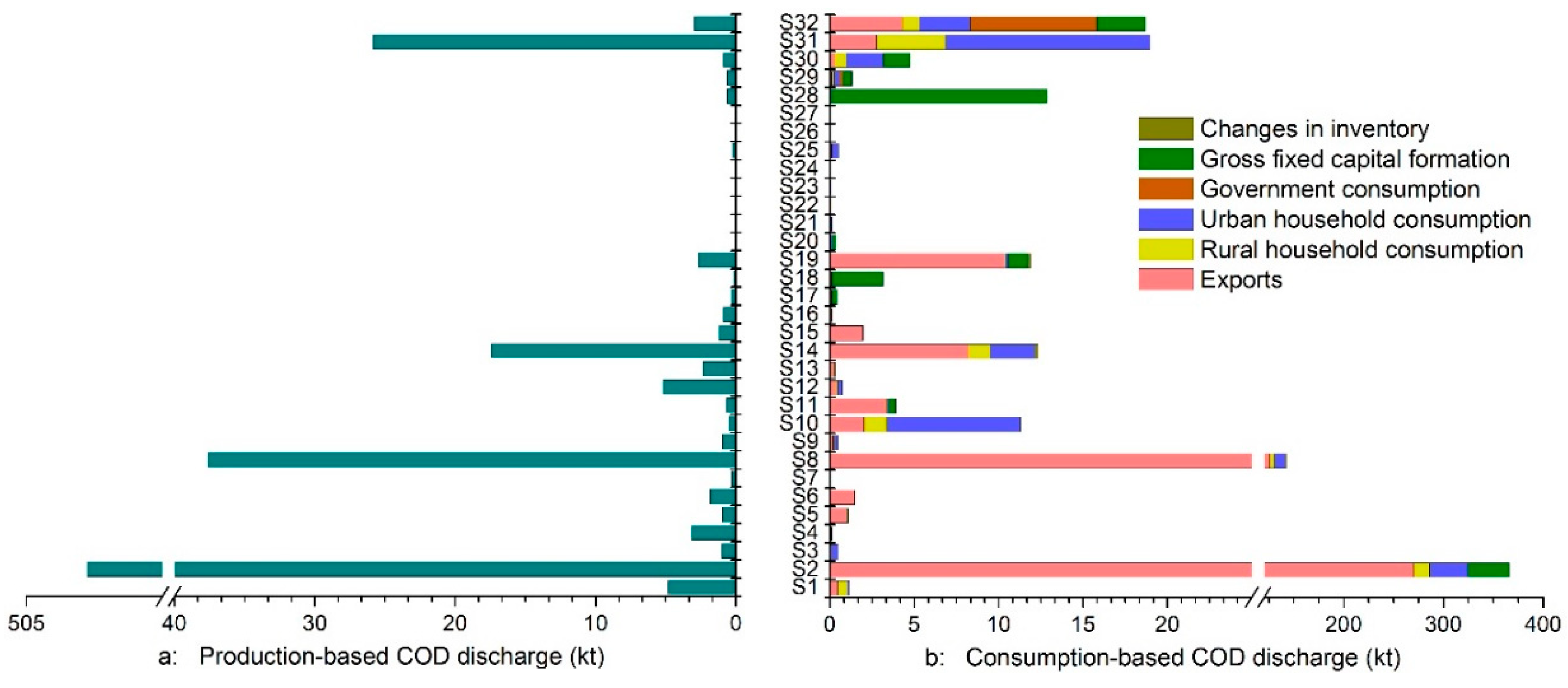
3.1. Consumption-Based Versus Production-Based COD Discharge

The local COD discharge is firstly measured from producer perspective (direct discharge in production process) by using production-based accounting method. Then it is estimated from consumer perspective by using consumption-based accounting method to generate the embodied COD discharge by sectors and final demand categories. Distributions of production-based versus consumption-based COD discharge are illustrated in Figure 1. The total local discharge of COD is 616.69 kt in 2012, among which Animal production (S2) contributes 81.53% and 59.26% from production-based and consumption-based views, respectively, followed by Foods & tobacco products (S8) and Hotels & catering services (S31). S2, S8, S31, and Chemical products (S14) are the main contributors, accounting for 94.56% of production-based COD discharge jointly. However, the direct sectoral COD discharge in the production process are re-allocated to sectors’ final demand, which makes S2, S8, S31, S14, Other services (S32), Construction (S28), Transport equipment (S19), and Clothing products (S10) the main contributors to consumption-based COD discharge. The embodied flows of COD discharge along the supply chains induce the disparities between production-based and consumption-based accountings. The consumption-based COD discharge of some sectors (such as S2, S14, and S31) decreases. The converse is illustrated in Figure 1, with S8, S10, S19, S28, Wholesale & retail trades (S30), and S32 as examples.

The embodied COD discharge instigated by final demand is clarified in Figure 1b. Exports induce the most embodied COD discharge, accounting for 70.23% of the total, followed by urban household consumption (12.92%), gross fixed capital formation (10.51), and rural household consumption (4.88%). For some specific sectors, exports are the dominant drivers for the embodied COD discharge of S2, S8, Sawmills & furniture (S11), S14, S19, and Nonmetallic mineral products (S15) with the contribution proportion ranging from 66.28% to 95.17%. The embodied COD discharge of S10, S30, and S31 are mainly contributed by urban household consumption with the contribution rates as 69.88%, 46.14%, and 63.97%, respectively. For Machinery (S18) and S28, gross fixed capital formation induces the most embodied COD discharge (96.17% and 99.34%, respectively). Government consumption is the main contributor for S32 with little influence on other sectors in terms of embodied COD discharge.

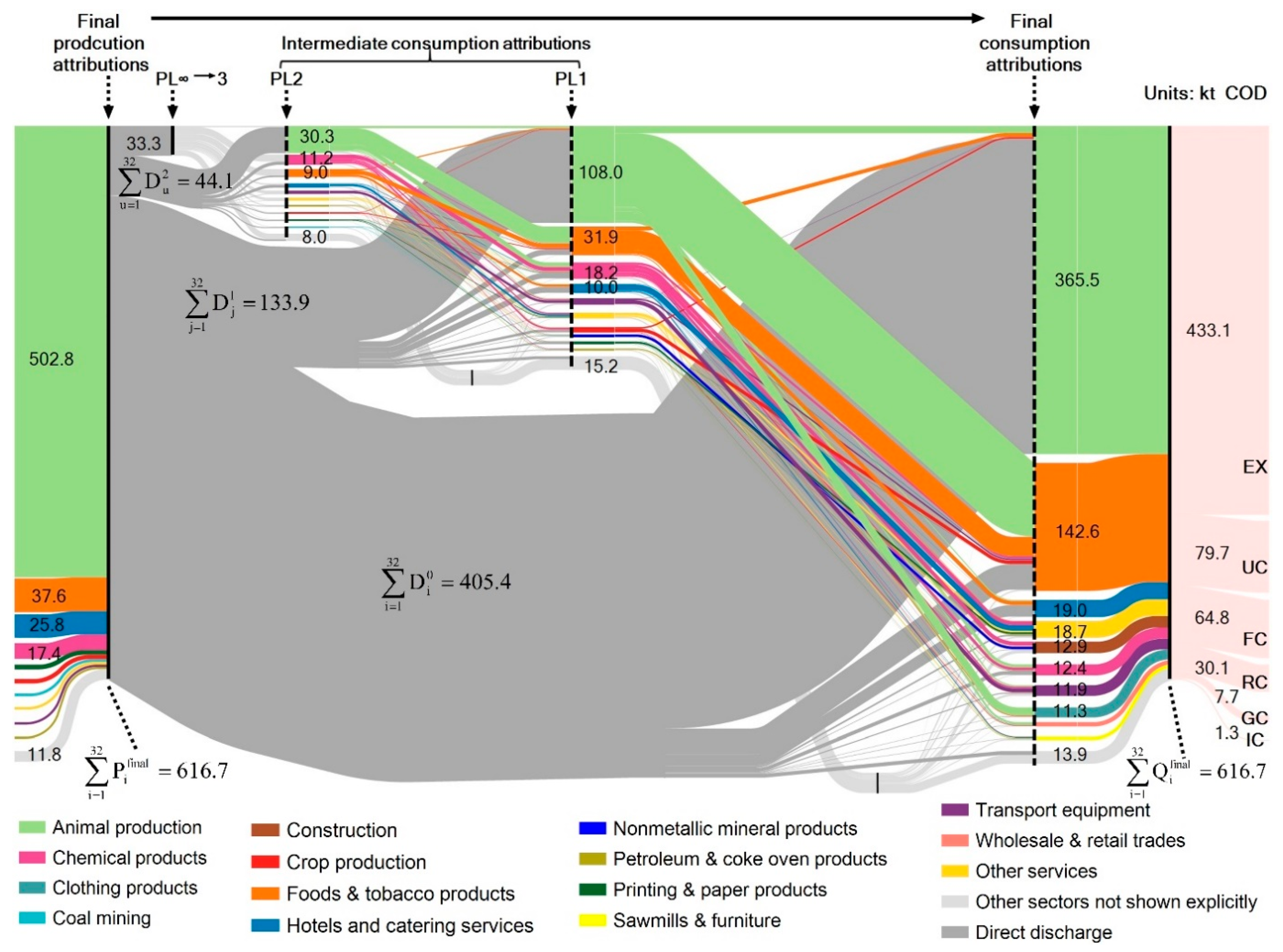
3.2. Embodied Flows of COD Discharge

SPA and mapping approach are collaboratively applied to investigate the disparities between production-based (final production attributions) and consumption-based (final consumption attributions) inventories of COD discharge. It is measured where the COD discharge from economic sectors has gone, and where the COD discharge embodied in final products has come from. Detailed information on direct and embodied COD discharges driven by the final demand purchases at layer 0 (PL⁰), layer 1 (PL¹), layer 2 (PL²), and layers ^3→∞ (PL^3→∞) is illustrated in Figure 2. A Sankey diagram follows the requirement of conservation of energy or mass from a physical view of production systems and illustrates the added value or costs of energy and material flows using flow charts [51]. Thus, it makes it possible to depict the embodied COD discharge through established connection between sectoral output and COD discharge. Three aspects of Sankey diagram are assumed in this study as: the diagrams concern quantity of COD discharge; the quantity scale uses the width of a flow chart; a mass balance (of COD discharge) is maintained. The COD discharge during the production of final products occurs at PL⁰. While, the COD discharge at other layers represent that induced during the production of the required inputs for the preceding adjacent layers. The embodied COD discharge flows across sectors and layers are also quantified in Figure 2. Most of the direct COD discharge occurs at PL⁰, accounting for 65.73% of the total, among which S2 is the dominant contributor (86.58%). This situation is different from the studies focusing on CO₂ and SO₂ emissions [6,17]. The rest of direct COD discharge occurring at higher layers is embodied in the products used as intermediate inputs, and is finally re-allocated to the sectors at PL⁰ through the supply chains. Figure 2 clarifies how the discrepancies between final production and consumption attributions of COD discharge generate. For example, S2 discharges 502.8 kt COD in the final production process. Some of the products of S2 are used as the intermediate inputs for other sectors. Thus, the embodied COD discharge in these products finally flows to other sectors such S8 and S10. However, the COD discharge embodied in the products used as the intermediate inputs for S2 to meet the final demand is less than the above outflow, which ultimately leads to the decrease of COD discharge in terms of final consumption accounting (365.5 kt). S8 has a converse situation compared with S2 (see Figure 2).

It is clear that the components of a sector’s embodied COD discharge in terms of final consumption attribution are different with others’ (Figure 2). The direct COD discharge of S2 at PL⁰ accounts for 96.04% (351.01 kt) of the embodied COD discharge. While, the remaining 3.96% is contributed by the required inputs from other sectors at PL¹. Conversely, for S8, the direct COD discharge at PL⁰ accounts for only 19.91% (28.39 kt), while the required inputs from PL¹ contributes 80.09%, with S2’s products accounting for 57.67%. Such a component analysis can be conducted for intermediate consumption attributions at higher layers. The COD discharge embodied in the inputs purchased from PL¹ can be further traced and decomposed into the induced direct COD discharge at layer 1, layer 2, and layer 3→ ∞ as shown in

Table 4. Distribution of direct COD discharge in production layers induced by final demand purchases.

Code	Sectors	Consumption-Based COD Discharge (kt)	Output (Billion CNY) a	Distribution of Induced Direct COD Discharges (%)
				Layer 0	Layer 1	Layer 2	Layer 3→ ∞
S2	Animal production	365.47	113.04	96.04	2.58	0.93	0.45
S8	Foods & tobacco products	142.58	362.82	19.91	61.02	12.92	6.15
S31	Hotels & catering services	18.98	62.74	67.06	12.55	14.88	5.51
S32	Other services	18.69	483.56	9.58	40.35	24.67	25.39
S28	Construction	12.89	288.83	4.87	23.14	32.38	39.61
S14	Chemical products	12.35	239.07	32.90	41.12	14.41	11.57
S19	Transport equipment	11.89	549.46	10.08	26.64	26.42	36.86
S10	Clothing products	11.28	18.27	3.72	80.32	10.61	5.35
S30	Wholesale & retail trades	4.77	148.53	11.37	60.63	13.06	14.95
S11	Sawmills & furniture	3.92	85.43	11.63	27.51	26.28	34.58
----	Other sectors	13.86	948.45	30.36	23.85	20.67	25.12

^a CNY denotes the Chinese Yuan.

. Direct COD discharge of S2 and S31 induced by final demand mostly occur at layer 0. While, only 3.72% and 4.87% COD discharge occur directly at layer 0 to meet the final demand of S10 and S28, respectively. For S8, S10, S14, S30, and S32, the direct COD discharge at layer 1 induced by final demand becomes the dominant contributor to the sector’s embodied COD discharge at final consumption attribution.

Figure 2 provides a holistic picture of sectoral embodied flows of COD discharge between producer and consumer. It also needs to investigate some major embodied flows of COD discharge through the supply chains. Thus, the paths with top-twelve contribution values for COD discharge are extracted as in

Table 5. The paths with top-twelve contribution values for COD discharge (starting from a final demand category and ending with a polluting production sector).

Rank	Layer	Contribution	Path
1	0	42.04%	Exports→ Animal production
2	1	11.29%	Exports→ Foods & tobacco products→ Animal production
3	0	6.52%	Gross fixed capital formation→ Animal production
4	0	5.93%	Urban household consumption→ Animal production
5	0	4.06%	Exports→ Foods & tobacco products
6	0	2.48%	Rural household consumption→ Animal production
7	2	2.20%	Exports→ Foods & tobacco products→ Foods & tobacco products→ Animal production
8	0	1.32%	Urban household consumption→ Hotels & catering services
9	1	1.01%	Urban household consumption→ Foods & tobacco products→ Animal production
10	1	0.96%	Urban household consumption→ Clothing products→ Animal production
11	1	0.93%	Exports→ Animal production→ Animal production
12	0	0.44%	Exports→ Chemical products

. These paths reveal how final demand drives COD discharge in the production process. The twelve paths collectively contribute to 79.18% of the overall COD discharge. Among them, exports drive the most COD discharge, accounting for 60.96%, followed by urban household consumption (9.22%). The path “Exports→ Animal production” accounts for 42.04% of the total COD discharge, followed by “Exports→ Foods & tobacco products→ Animal production” (11.29%) and “Gross fixed capital formation→ Animal production” (6.52%). Nine of the top-twelve paths end up with Animal production (S2). Foods & tobacco products (S8) appears in four paths. S2 and S8 are the two key sectors for formulating COD reduction policies and measures. Seven paths end at layer 0, indicating that the end-of-pipe COD discharge from these sectors (S2, S8, and S14) are not well controlled.

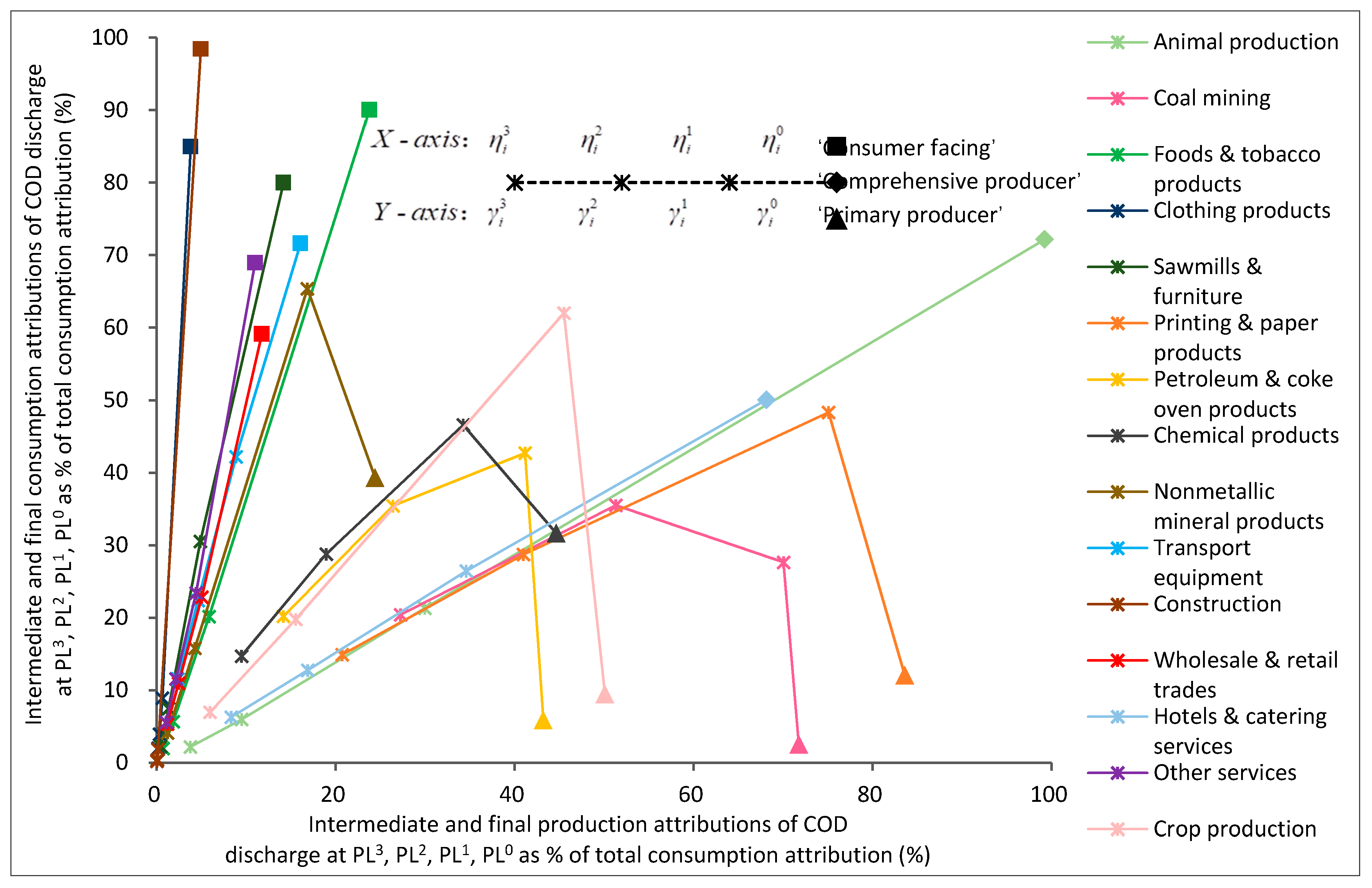
3.3. Normalized Evolution of Consumption and Production Attributions

Equations (10)–(12) are used to calculate the proportions of a sector’s intermediate production and consumption attributions at PL¹, PL², and PL³ and final (PL⁰) production and consumption attributions in its total consumption attribution. The normalized results are presented in Figure 3. Final consumption attributions (at PL⁰, the end of lines) of Clothing products (S10), Construction (S28), Sawmills & furniture (S11), and Foods & tobacco products (S8) account for more than 80% of their total consumption attributions. For Animal production (S2) and Printing & paper products (S12), the same situation happens to final production attribution. Other sectors’ final production and consumption attributions both contribute less than 80% of their total consumption attributions. For example, final consumption and production attributions of Nonmetallic mineral products (S15) account for 39.29% and 24.4% of its total consumption attribution, respectively. Therefore, only an analysis of a sector’s final consumption and production attributions is insufficient to identify its overall impact.

In order to clarify where the overall impact of a sector’s COD discharge concentrates in the production system, a sector’s evolution of consumption and production attributions can be unfolded with the assistance of Figure 3 [6]. The difference between the points at PL⁰ and PL¹ (read off the x-axis) is large for Animal production (S2), indicating that a large quantity of direct COD discharge appears at PL⁰. This part of direct COD discharge contributes to 69.29% of the total consumption attribution. It can be concluded that the overall impact of COD discharge for S2 greatly concentrates at PL⁰. For Printing & paper products (S12), a large share of total direct COD discharge appears at PL¹. This part of direct COD discharge accounts for 34.11% of the total consumption attribution and contributes to 40.59% of the normalized intermediate consumption attribution at PL¹. Different from S2, a sudden decrease in consumption attribution from PL¹ to PL⁰ occurs for S12, indicating that some of S12’s products are consumed by final demand. The overall impact of COD discharge of S12 relatively concentrates at PL¹ due to the direct COD discharge at PL¹. For another example, Petroleum & coke oven products (S13) is focused on. A similar sudden decrease happens to S13 compared with S12 but accompanied by a slight increase in the production attribution. Therefore, the overall impact of COD discharge is not observably enhanced at PL⁰. Furthermore, direct COD discharge from PL¹ and PL² accounts for a small proportion of the normalized consumption attribution. Each final or intermediate attribution contributes to less than 45% of the total consumption attribution. Thus the overall impact of COD discharge does not concentrate at any layer. For S13, both the upstream COD discharge from other sectors and direct COD discharge are considerable.

As delineated in Figure 3, three groups of sectors can be determined based on the characteristics of the evolution of sectors’ normalized consumption and production attributions of COD discharge [6]. The sectors with a sudden jump in their consumption attribution and a small production attribution at PL⁰ are defined as “consumer facing”, such as Construction (S28), Foods & tobacco products (S8), and sawmills & furniture (S11). These sectors mainly provide products to final demand, directly. While, Petroleum & coke oven products (S13), Coal mining (S4), and Printing & paper products (S12) are involved in the “primary producer” group, considering that these sectors have a small increase in their production attribution and a sudden drop in their consumption attribution at PL⁰. These sectors mainly provide products as intermediated inputs for other sectors. As a “comprehensive producer” sector, Animal production (S2) has a continuously increasing trend in consumption and production attributions of COD discharge through four layers, and provides products to meet both intermediate and final demands.

4. Discussion and Policy Implications

Production-based and consumption-based accountings have been applied to estimate the COD discharged into local water environment in sector-level and final demand category-level. The former is adept at investigating direct COD discharge in the production process, and the latter makes it possible to monitor the COD discharge induced by final demand. The results from the two aspects facilitate to formulate the policies for controlling COD discharge from different perspectives. The much larger direct COD discharge intensity plus relatively higher output (see Figure A1) make Animal production (S2) the dominant contributor to total direct COD discharge. As a base of livestock and poultry breeding in China [4], Jilin Province should make efficient policies to promote the utilization of livestock and poultry excrements for fertilizer production and biomass power generation, and implement centralized breeding patterns to reduce COD discharge [8]. From the consumption perspective, the COD discharged into Jilin Province is mainly driven by exports of products (70.23%). Furthermore, S2 and Foods & tobacco products (S8) account for 62.32% and 29.02% of COD discharge embodied in products for exports, respectively. Thus, cutting capacity of S2 and S8 should be significant for COD discharge control.

Differences between final production and consumption attributions of COD discharge have been revealed (Figure 1). Clarification of sectoral interdependences in terms of COD discharge within the IO framework provides foundation supports on revealing how the differences arise. SPA and mapping approach built on IO models successfully solve the issue by identifying direct COD discharge at each layer and tracing the transmission of COD discharge embodied in intermediate products across sectors and layers. Then, the quantitative and diagrammatic results obtained may help to facilitate industrial restructuring for COD discharge control. Foods & tobacco products (S8) only accounts for 6.10% of total direct COD discharge in the production process, however, drives 18.52% of total final consumption attribution of COD discharge (by purchasing intermediate products provide by the upstream sectors) (see Figure 2), such as Animal production (S2) and Foods & tobacco products (S8). Therefore, in order to reduce S8’s final consumption attribution of COD discharge, the COD discharge intensity of the upstream sectors (S2) should be lowered and S8’s product structure should be adjusted by increasing the proportion of intermediate materials with relatively lower embodied COD discharge. Sawmills & furniture (S11), Construction (28), and Clothing products (S10) share similar situation compared with S8. S2, a COD discharge-intensive sector, provides other sectors such as S10, S8, and Chemical products (S14) with intermediate products. The production of these sectors can be cut down, which is an alternative way to reduce COD discharge.

Identification of the key sectors and paths in terms of COD discharge are critical for formulating specific policies and measures. Animal production (S2) and Foods & tobacco products (S8) are the two key sectors in the economy of Jilin Province. It’s a priority to promote innovations of production technologies and improvement of end-of-pipe abetment abilities for these two sectors. Simultaneously, as exports instigate a large quantity of COD discharge embodied in the products of S2 and S8 in some key paths, it is urgent to cut the production capacity or reduce the investment on S2 and S8, and finally reduce the exports of their products. Clothing products (S10) and Chemical products (S14) are relatively less important compared with S2 and S8. Cutting production capacities of the key sectors will affect the production of the downstream sectors, which can lead to industrial restructuring. However, policymaking should also focus on encouraging the development of the sectors with lower COD discharge intensity and less requirement for COD discharge-intensive products as intermediate inputs.

Evolution of normalized consumption and production attributions of COD discharge makes it possible to clarify where the overall impact of a sector’s COD discharge concentrates. It also provides detailed information on the distribution of upstream COD discharge from other sectors and direct COD discharge at each layer. Furthermore, three groups of sectors can be categorized to judge whether a sector mainly provides products to meet intermediate demand, final demand or both. This novel approach can be applied to compare the characteristics and impacts of sectoral emissions/discharge across cities, regions, and nations. Once the time-series IO tables can be obtained, this approach is also capable of depicting the changes in the impacts of a sector’s energy/resources use or emissions within a certain time horizon.

5. Conclusions

Jilin Province, as an undeveloped and water pollution intensive region in China, is chosen as the empirical study area to investigate the water pollutant (with COD as the water pollutant indicator) discharge linked to the production and consumption activities in 2012. The production-based and consumption-based accounting methods based on the input–output framework are used to measure direct COD discharge in the production process and COD discharge embodied in final products. SPA and mapping approach are jointly used to trace the embodied flows of COD discharge through the supply chains, which can clarify how the discrepancies of COD discharge from production and consumption perspectives arise. Additionally, the normalized consumption and production attributions are estimated to reveal where the overall impact of a sector’s COD discharge concentrates.

The empirical results reveal that Animal production (S2) is the dominant contributor to local total COD discharge from both production and consumption perspectives, followed by Foods & tobacco products (S8). 70.23% of the total COD discharge is driven by exports. The direct COD discharge directly triggered by final demand accounts for 65.73% of the total, with the rest induced through the supply chains. The components of sectors’ COD discharge at final consumption attribution are different. The COD discharge driven by S8, Sawmills & furniture (S11), and Construction (28) mainly occurs at higher production layers. While, the direct COD discharge of S2 at layer 0 accounts for 96.04% of its final consumption attribution of COD discharge. The key sectors and key paths in terms of COD discharge have been extracted. The top 1 path is “Exports→Animal production” which drives 42.04% of COD discharge. S2 and S8 are the two key sectors in the supply chains. As a COD discharge-intensive sector, S2 provides intermediate products to other sectors, which drives the downstream sectors’ final consumption attributions of COD discharge to increase significantly.

Based on the above findings, some countermeasures can be proposed to control COD discharge for Jilin Province. It’s a priority to promote innovations of production technologies and improvement of end-of-pipe abetment abilities for S2 and S8. Resource and energy oriented utilization of livestock and poultry excrements should also be impelled. Industrial restructuring should be propelled via cutting production capacity or reducing investment on S2 and S8. Export of S2’s products should be largely cut down, coupled with the adjustment of the export structure. Simultaneously, development of the sectors with lower embodied (direct plus indirect) water pollutant discharge intensity should be encouraged. The findings of this study can give reference to other undeveloped regions where livestock and poultry industry contributes to the water pollutant discharge the most remarkably. More importantly, the approach used in this study can be applied to other regions or nations for analyzing the integrated energy-environmental-economic system and clarifying how energy, water resource, emissions, discharges etc. “flow” in the production system. The analytical results obtained should help to formulate policies from multiple perspectives for emissions control.

References

1. World Water Assessment Programme. The United Nations World Water Development Report 2015; Water for a Sustainable World; UNESCO: Paris, France, 2015; pp. 2–6. [Google Scholar]
2. Voeroesmarty, C.J.; McIntyre, P.B.; Gessner, M.O.; Dudgeon, D.; Prusevich, A.; Green, P.; Glidden, S.; Bunn, S.E.; Sullivan, C.A.; Liermann, C.R.; et al. Global threats to human water security and river biodiversity. Nature 2010, 467, 555–561. [Google Scholar] [CrossRef] [PubMed]
3. Liu, J.; Yang, W. Water Sustainability for China and Beyond. Science 2012, 337, 649–650. [Google Scholar] [CrossRef] [PubMed]
4. Yang, W.; Song, J.; Higano, Y.; Tang, J. Exploration and assessment of optimal policy combination for total water pollution control with a dynamic simulation model. J. Clean. Prod. 2015, 102, 342–352. [Google Scholar] [CrossRef]
5. Yang, W.; Song, J.; Higano, Y.; Tang, J. An Integrated Simulation Model for Dynamically Exploring the Optimal Solution to Mitigating Water Scarcity and Pollution. Sustainability 2015, 7, 1774–1797. [Google Scholar] [CrossRef] [Green Version]
6. Skelton, A.; Guan, D.; Peters, G.P.; Crawford-Brown, D. Mapping Flows of Embodied Emissions in the Global Production System. Environ. Sci. Technol. 2011, 45, 10516–10523. [Google Scholar] [CrossRef]
7. Yang, W.; Song, J.; Higano, Y.; Tang, J. Combination of Assessment Indicators for Policy Support on Water Scarcity and Pollution Mitigation. Water 2016, 8, 203. [Google Scholar] [CrossRef]
8. Song, J.; Yang, W.; Li, Z.; Higano, Y.; Wang, X. Discovering the energy, economic and environmental potentials of urban wastes: An input–output model for a metropolis case. Energy Convers. Manag. 2016, 114, 168–179. [Google Scholar] [CrossRef]
9. Peters, G.P.; Hertwich, E.G. Structural analysis of international trade: Environmental impacts of Norway. Econ. Syst. Res. 2006, 18, 155–181. [Google Scholar] [CrossRef]
10. Bagheri, M.; Guevara, Z.; Alikarami, M.; Kennedy, C.A.; Doluweera, G. Green growth planning: A multi-factor energy input-output analysis of the Canadian economy. Energy Econ. 2018, 74, 708–720. [Google Scholar] [CrossRef]
11. Guan, D.; Hubacek, K.; Tillotson, M.; Zhao, H.; Liu, W.; Liu, Z.; Liang, S. Lifting China’s water spell—SDA. Environ. Sci. Technol. 2014, 48, 11048–11056. [Google Scholar] [CrossRef]
12. Liang, S.; Wang, Y.; Zhang, C.; Xu, M.; Yang, Z.; Liu, W.; Liu, H.; Chiu, A.S.F. Final production-based emissions of regions in China. Econ. Syst. Res. 2018, 30, 18–36. [Google Scholar] [CrossRef]
13. Leontief, W. Environmental repercussions and the economic structure: An input-output approach. Rev. Econ. Stat. 1970, 52, 262–271. [Google Scholar] [CrossRef]
14. Davis, S.J.; Caldeira, K. Consumption-based accounting of CO2 emissions. Proc. Natl. Acad. Sci. USA 2010, 107, 5687–5692. [Google Scholar] [CrossRef] [PubMed]
15. Erickson, P.; Allaway, D.; Lazarus, M.; Stanton, E.A. A Consumption-Based GHG Inventory for the U.S. State of Oregon. Environ. Sci. Technol. 2012, 46, 3679–3686. [Google Scholar] [CrossRef] [PubMed]
16. Zhao, H.Y.; Zhang, Q.; Guan, D.B.; Davis, S.J.; Liu, Z.; Huo, H.; Lin, J.T.; Liu, W.D.; He, K.B. Assessment of China’s virtual air pollution transport embodied in trade by using a consumption-based emission inventory. Atmos. Chem. Phys. 2015, 15, 5443–5456. [Google Scholar] [CrossRef]
17. Meng, J.; Liu, J.; Xu, Y.; Tao, S. Tracing Primary PM2.5 emissions via Chinese supply chains. Environ. Res. Lett. 2015, 10, 054005. [Google Scholar] [CrossRef]
18. Peters, G.P.; Hertwich, E.G. Post-Kyoto greenhouse gas inventories: Production versus consumption. Clim. Chang. 2008, 86, 51–66. [Google Scholar] [CrossRef]
19. Peters, G.P. From production-based to consumption-based national emission inventories. Ecol. Econ. 2008, 65, 13–23. [Google Scholar] [CrossRef]
20. Huo, H.; Zhang, Q.; Guan, D.; Su, X.; Zhao, H.; He, K. Examining Air Pollution in China Using Production- And Consumption-Based Emissions Accounting Approaches. Environ. Sci. Technol. 2014, 48, 14139–14147. [Google Scholar] [CrossRef]
21. Franzen, A.; Mader, S. Consumption-based versus production-based accounting of CO2 emissions: Is there evidence for carbon leakage? Environ. Sci. Technol. 2018, 84, 34–40. [Google Scholar] [CrossRef]
22. Karakaya, E.; Yilmaz, B.; Alatas, S. How production-based and consumption-based emissions accounting systems change climate policy analysis: The case of CO2 convergence. Environ. Sci. Poll. Res. 2019, 26, 16682–16694. [Google Scholar] [CrossRef] [PubMed]
23. Lenzen, M.; Kanemoto, K.; Moran, D.; Geschke, A. Mapping the Structure of the World Economy. Environ. Sci. Technol. 2012, 46, 8374–8381. [Google Scholar] [CrossRef] [PubMed]
24. Wang, Z.; Cui, C.; Peng, S. Critical sectors and paths for climate change mitigation within supply chain networks. J. Environ. Manag. 2018, 226, 30–36. [Google Scholar] [CrossRef] [PubMed]
25. Li, Y.; Su, B.; Dasgupta, S. Structural path analysis of India’s carbon emissions using input-output and social accounting matrix frameworks. Energy Econ. 2018, 76, 457–469. [Google Scholar] [CrossRef]
26. Lenzen, M. Structural path analysis of ecosystem networks. Ecol. Model. 2007, 200, 334–342. [Google Scholar] [CrossRef]
27. Hanaka, T.; Kagawa, S.; Ono, H.; Kanemoto, K. Finding environmentally critical transmission sectors, transactions, and paths in global supply chain networks. Energy Econ. 2017, 68, 44–52. [Google Scholar] [CrossRef]
28. Lenzen, M. Structural analyses of energy use and carbon emissions—An overview. Econ. Syst. Res. 2016, 28, 119–132. [Google Scholar] [CrossRef]
29. Zhang, B.; Qu, X.; Meng, J.; Sun, X. Identifying primary energy requirements in structural path analysis: A case study of China 2012. Appl. Energy 2017, 191, 425–435. [Google Scholar] [CrossRef] [Green Version]
30. Hong, J.; Shen, Q.; Xue, F. A multi-regional structural path analysis of the energy supply chain in China’s construction industry. Energy Policy 2016, 92, 56–68. [Google Scholar] [CrossRef]
31. Zhang, B.; Guan, S.; Wu, X.; Zhao, X. Tracing natural resource uses via China’s supply chains. J. Clean. Prod. 2018, 196, 880–888. [Google Scholar] [CrossRef]
32. Wang, J.; Du, T.; Wang, H.; Liang, S.; Xu, M. Identifying critical sectors and supply chain paths for the consumption of domestic resource extraction in China. J. Clean. Prod. 2019, 208, 1577–1586. [Google Scholar] [CrossRef]
33. Shao, L.; Li, Y.; Feng, K.; Meng, J.; Shan, Y.; Guan, D. Carbon emission imbalances and the structural paths of Chinese regions. Appl. Energy 2018, 215, 396–404. [Google Scholar] [CrossRef] [Green Version]
34. Oshita, Y. Identifying critical supply chain paths that drive changes in CO2 emissions. Energy Econ. 2012, 34, 1041–1050. [Google Scholar] [CrossRef]
35. Gui, S.; Mu, H.; Li, N. Analysis of impact factors on China’s CO2 emissions from the view of supply chain paths. Energy 2014, 74, 405–416. [Google Scholar] [CrossRef]
36. Skelton, A. EU corporate action as a driver for global emissions abatement: A structural analysis of EU international supply chain carbon dioxide emissions. Glob. Environ. Chang. Hum. Policy 2013, 23, 1795–1806. [Google Scholar] [CrossRef]
37. Lenzen, M. Environmentally important paths, linkages and key sectors in the Australian economy. Struct. Chang. Econ. Dyn. 2003, 14, 1–34. [Google Scholar] [CrossRef]
38. Zhang, Q.; Nakatani, J.; Shan, Y.; Moriguchi, Y. Inter-regional spillover of China’s sulfur dioxide (SO2) pollution across the supply chains. J. Clean. Prod. 2019, 207, 418–431. [Google Scholar] [CrossRef]
39. Nagashima, F.; Kagawa, S.; Suh, S.; Nansai, K.; Moran, D. Identifying critical supply chain paths and key sectors for mitigating primary carbonaceous PM2.5 mortality in Asia. Econ. Syst. Res. 2016, 29, 105–123. [Google Scholar] [CrossRef]
40. Llop, M.; Ponce-Alifonso, X. Identifying the role of final consumption in structural path analysis: An application to water uses. Ecol. Econ. 2015, 109, 203–210. [Google Scholar] [CrossRef] [Green Version]
41. Wu, F.; Sun, Z.; Wang, F.; Zhang, Q. Identification of the critical transmission sectors and typology of industrial water use for supply-chain water pressure mitigation. Resour. Conserv. Recycl. 2018, 131, 305–312. [Google Scholar] [CrossRef]
42. Wiedmann, T.; Lenzen, M.; Turner, K.; Barrett, J. Examining the global environmental impact of regional consumption activities—Part 2: Review of input-output models for the assessment of environmental impacts embodied in trade. Ecol. Econ. 2007, 61, 15–26. [Google Scholar] [CrossRef]
43. Sonis, M.; Guilhoto, J.J.M.; Hewings, G.J.D.; Martins, E.B. Linkages, Key Sectors and Structural Change: Some New Perspectives. Dev. Econ. 1995, 33, 233–270. [Google Scholar] [CrossRef]
44. Weber, C.L.; Peters, G.P.; Guan, D.; Hubacek, K. The contribution of Chinese exports to climate change. Energy Policy 2008, 36, 3572–3577. [Google Scholar] [CrossRef] [Green Version]
45. Zhao, X.; Yang, H.; Yang, Z.; Chen, B.; Qin, Y. Applying the Input-Output Method to Account for Water Footprint and Virtual Water Trade in the Haihe River Basin in China. Environ. Sci. Technol. 2010, 44, 9150–9156. [Google Scholar] [CrossRef] [PubMed]
46. Guan, D.; Su, X.; Zhang, Q.; Peters, G.P.; Liu, Z.; Lei, Y.; He, K. The socioeconomic drivers of China’s primary PM2.5emissions. Environ. Res. Lett. 2014, 9, 024010. [Google Scholar] [CrossRef]
47. Editorial Committee of China Environment Book. China Environment Book 2013; Society of China Environment Book Press: Beijing, China, 2013. (In Chinese) [Google Scholar]
48. National Bureau of Statistics. China Statistical Yearbook on Environment 2013; China Statistics Press: Beijing, China, 2013. (In Chinese)
49. Wang, X.; Huang, K.; Yu, Y.; Hu, T.; Xu, Y. An input–output structural decomposition analysis of changes in sectoral water footprint in China. Ecol. Indic. 2016, 69, 26–34. [Google Scholar] [CrossRef]
50. Statistics Bureau of Jilin. Jilin Statistical Yearbook 2013; China Statistics Press: Beijing, China, 2013. (In Chinese)
51. Schmidt, M. The Sankey diagram in energy and material flow management—Part II: Methodology and current applications. J. Ind. Ecol. 2008, 12, 173–185. [Google Scholar] [CrossRef]
Figure 1. Sectoral distributions of production-based (a) and consumption-based (b) CDO discharges.
Sustainability 11 03774 g001
Figure 2. Sankey diagram of embodied flows of COD discharge across economic sectors. The flows start from the left side and end at the right side. The width of each flow denotes the magnitude of COD discharge (unit: kt). The left side, central part, and right side of the diagram represent final production, intermediate consumption (PL1 and PL2), and final consumption attributions of COD discharge. The top-ten sectors for COD discharge are shown individually at the stages of final production, intermediate and final consumption attributions, while the remaining sectors are combined as one group. The dark gray flows starting from final production attribution depicts the direct COD discharge at PL0, PL1, and PL2. The PL0 and PL1 layers are connected by embodied flows of COD discharge, the same for PL1 and PL2 layers. The pink flows on the right side of the diagram represent the COD discharge driven by final demand. EX, UC, FC, RC, GC, and IC denote exports, urban household consumption, gross fixed capital formation, rural household consumption, government consumption, and changes in inventory, respectively.
Sustainability 11 03774 g002
Figure 3. Evolution of sectoral production and consumption attributions of COD discharge from PL3 to PL0 normalized as the percentage of sectoral total consumption attribution. The line starts from the point at PL3 and ends at PL0 (from left to right, from bottom to top). A sector’s proportions of final production attribution (PL0, X-axis) and final consumption attribution (PL0, Y-axis) in sector total consumption attribution are illustrated by the solid markers at the end of each line. A sector’s proportions of intermediate production and consumption attributions at PL3, PL2, and PL1 in sector total consumption attribution are indicated by the star markers. η i t and γ i t (t = 0, 1, 2, 3, represents the layers) denote the percentage of a sector’s final and intermediate production attributions and final and intermediate consumption attributions in its total consumption attribution, respectively Equation (12). Solid lines connecting the data points are shown to aid the visual inspection of discrete measurements and do not represent a continuous series.
Sustainability 11 03774 g003