Financial Structure and Systemic Risk of Banks: Evidence from Chinese Reform

Abstract

Using Chinese data from 2006 to 2014, we find that a shift in the financial structure towards a more market-based structure can reduce the systemic risk of the banking sector. One transmission channel through which this occurs is the improvement in an individual firm’s debt repaying capacity, which is positively influenced by the development of stock markets. Another channel is the enhanced credit monitoring of borrowers by banks, owing to their slower credit growth. Our results imply that the shift toward market-based financial structure could lead to the development of financial market as well as the enhancement of the stability of an economy.

1. Introduction

The recent financial crises have imparted a number of negative consequences on the real economy in the US and the world as a whole. Specifically, the effects of the 2007–2008 global financial crisis and the 2011 European sovereign debt crisis on the global economy resulted in a large number of bank failures. The economic recession that followed the crises alerted that systemic bank failures could have devastating impacts on economic and social stability. Due to this series of events, the systemic risk of the banking sector began to draw the attention of academics as well as policy makers.

The systemic risk of the banking sector generally refers to the potential risk of system breakdown due to the interconnection among financial institutions. Specifically, Engle et al. [1] defined systemic risk as the propensity of an individual financial institution to be under-capitalized when the financial structure as a whole is under-capitalized. The authors also reported that, in Europe, a traditionally bank-based economy, banks account for nearly 80% of the total systemic risk. Our study investigates whether the systemic risk of the banking sector can be reduced if the financial structure becomes more market-based, relying less on traditional bank financing. Financial structure can be classified as bank-based or market-based, and the literature is inconclusive with regard to the relative advantages of each system. This study contributes to the debate on bank-based versus market-based structure from the perspective of the relative systemic risk of the banking sector.

One stream of the literature has highlighted the merits of a bank-based financial structure. For example, banks can finance industrial expansion more effectively than markets in emerging economies, and state-owned banks can overcome market failures and funnel domestic savings to strategically important projects [2]. A bank-based structure is more effective for new innovative activities because banks can credibly supply additional funds during projects [3]. However, the opposite view focuses on the inefficient allocation of capital in a bank-based financial structure. Banks have an inherent bias toward conservative investments; thus, they are likely to avoid funding innovative projects [4], and powerful banks frequently impede innovation by extracting informational rent and protecting established firms [5,6]. State-owned banks are more inclined to supply credit to labor-intensive industries rather than strategic industries, where possible innovation and opportunities exist for growth [7]. In addition, market-based economies have shown significantly stronger recovery than bank-based economies following a crisis [8]. An expansion of banking system relative to markets is linked to higher systemic risk and slower economic growth [9], and the service provided by banking sector becomes relatively less important than those provided by markets as economies grow [10]. Finally, some literature has documented that banks and markets are irrelevant and complementary to each other for economic growth [11,12]. Thus, the overall development of the financial structure, through developing several financing channels, is more important for enhancing capital allocation [13,14,15,16]. In this perspective, reduction in information asymmetry and/or transaction costs and an improvement in the legal efficiency are the primary issues; thus, whether the financial structure is bank-based or market-based would not matter [13,17].

To the best of our knowledge, this study is one of the early papers to directly examine the relationship between the financial structure of an economy and the systemic risk of the banking sector. In this work, we attempt to answer the following questions: (1) Did a shift from bank-based financial structure to market-based financial structure in the Chinese economy reduce the systemic risk of the banking sector? (2) If so, what are the transmission channels?

To answer these questions, this study employs two important approaches that are distinct from those used in previous studies. First, our study uses data from the Chinese banking sector. The Chinese government led the rapid shift in its financial structure, which had been dominated by the banking sector [18], towards a market-based structure. In 2004, the government proposed, for the first time, that China should vigorously develop security markets and increase the proportion of market-based financing in the economy. The 11th five-year plan, proclaimed at the People’s Congress in 2006, required an increase in the proportion of market financing and placed an emphasis on developing security markets. The third Plenary Session of the 18th Central Committee of the Communist Party of China in 2013 further emphasized the need to increase the proportion of security markets in the financial structure. In 2014, the government again accentuated the healthy development of equity and bond markets. Meanwhile, the Chinese banking sector is considered to have potential risk even without any bank default. The Chinese government provided several aid packages to banks to reduce the potential risk. For instant, Industrial and Commercial Bank of China (ICBC) received capital of 15 billion USD in April 2005, and capital of 19 billion USD was given to Agricultural Bank of China (ABC) in November 2008. Four state-owned asset management companies were established in 1999 to take over the non-performing loans (NPLs) worth 1.4 trillion RMB from the Big Four banks—Bank of China (BoC), China Construction Bank (CCB), ICBC and ABC—at their face value. Thus, the Chinese banking sector provides a noble experimental setting to examine the association between changes in the financial structure and the systemic risk of the banking sector.

Second, we use a market-based approach to measure the systemic risk of the banking sector due to the limitations associated with the traditional accounting measures that are widely used in the literature. Accounting measures of the systemic risk of the banking sector heavily rely on the financial statements of banks, such as the NPL ratio, earnings, profitability, and asset liquidity. Because accounting statements are reported with a delay and only measured quarterly, accounting measures of the systemic risk do not include real-time or short-term risk measurement [19,20,21]. Furthermore, accounting-based measures are exposed to the manipulation and amendment of accounting principles. The unique definition of NPLs in China is another reason why market-based measures are used. The Chinese definition of NPLs excludes low-quality loans transferred to state-owned asset management companies; thus, NPLs of Chinese banks are underestimated [18]. In addition, market-based risk measures could reflect the risk of the fast-growing shadow banking industry in China, while accounting-based measures cannot, due to the off-balance sheet nature of the business [22]. The size of China’s shadow banking system was estimated as ranging from 13.7 trillion RMB to 30 trillion RMB during 2012–2013. This is about 14–31% of the aggregate assets of Chinese banks and approximately 26–57% of the GDP in 2012 [22]. Assessing the systemic risk of the banking sector based on accounting measures would result in an underestimation of the true insolvency risk of the banking sector.

The market-based systemic risk has been widely employed in academic research, because market information can capture the inter-connections between banks that are not shown in banks’ financial statements [23]. For instance, equity return data were used to calculate the systemic risk, defined as the probability of a given number of simultaneous bank defaults [24]. The Nth-to-default probability, which indicates the probability of observing an Nth default among different financial institutions, used credit default swaps to measure the systemic risk, because price changes reflect the anticipation of future price movement [19,20]. Specifically, Merton’s approach has been widely applied for the evaluation of an individual bank’s risk, assessment of credit risk, and pricing deposit insurance [25,26,27]. Merton’s Value at Risk (VaR) framework was utilized to examine the relationship between systemic risk, GDP growth, the bank equity index and inflation rate [28], and the interactions between default, credit growth, and asset prices in the banking sector of 17 countries [29].

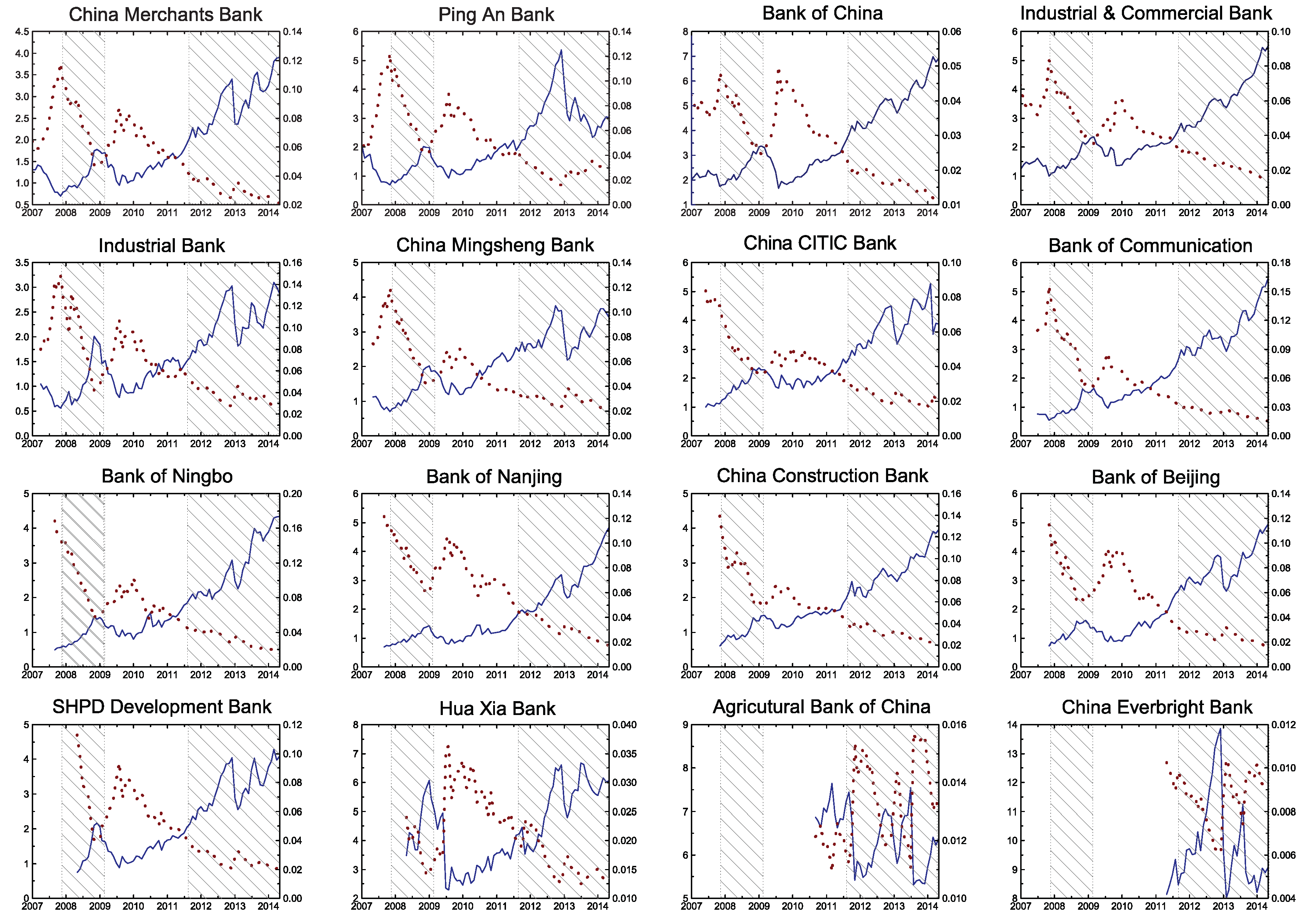
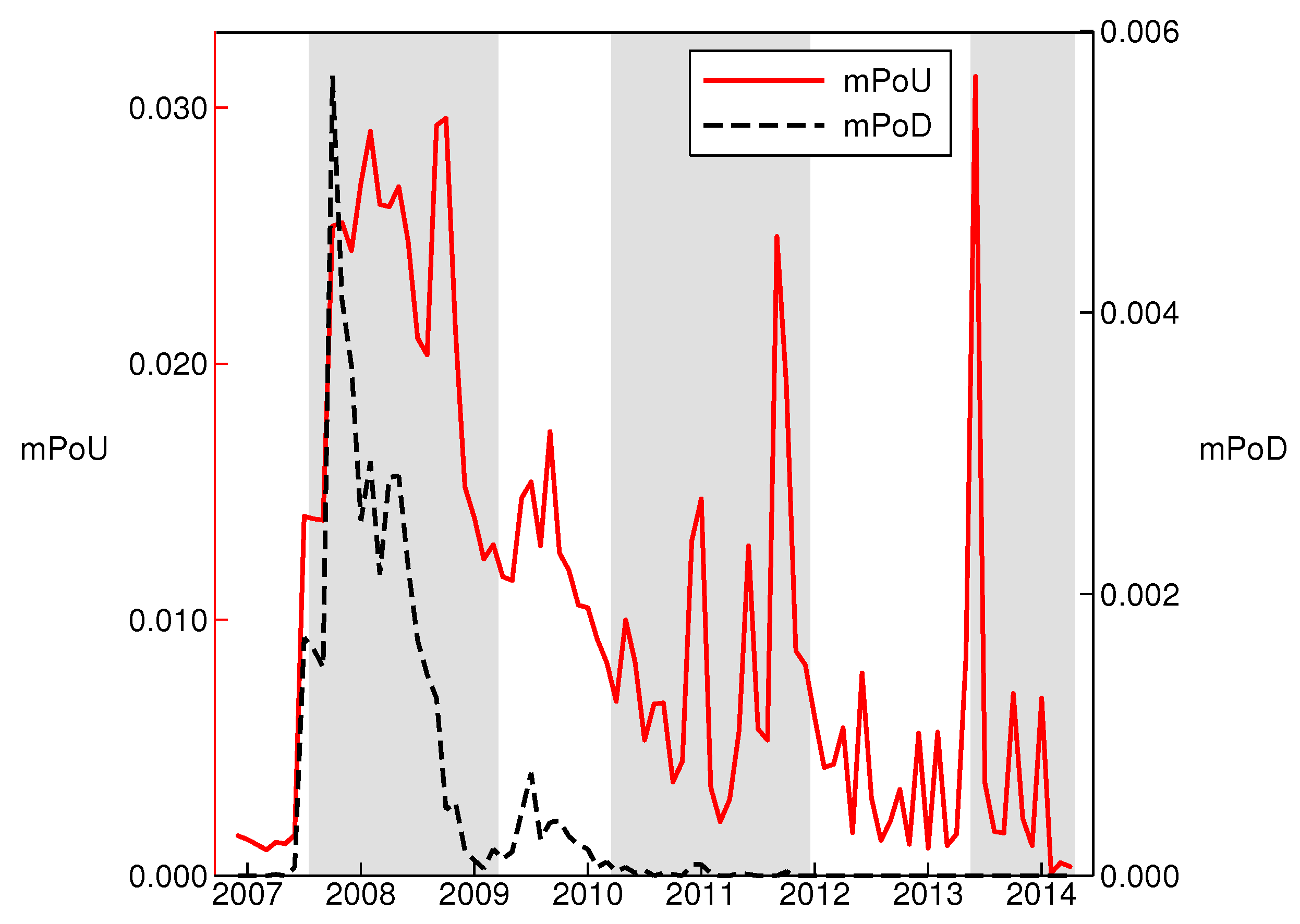
We adopt multiple probability of under-capitalization (mPoU), the aggregation of an individual bank’s probability of under-capitalization (PoU), as the measure of the systemic risk of the banking sector. PoU is conceptually similar to the better-known probability of default (PoD), but with several advantages. Banks are subject to maintain a certain capital adequacy ratio (CAR); thus, under-capitalization is a more imminent threat to banks than default. PoU includes the minimum capital reserve in its calculation, but PoD does not. Furthermore, mPoU takes financial contagion into account through asset correlation in the banking sector. It is essential to do this when measuring the systemic risk of the banking sector because a small shock of an individual bank, originally affecting only a few financial institutions, can easily spread to other banks and put the whole banking system at risk [30,31].

Our empirical study first shows that the market-based measure of the systemic risk of the banking sector in China is lower when the financial structure becomes more market-based. This perhaps indicates the effort of the Chinese government to promote a more market-based financial structure paid off by lowering the systemic risk of the banking sector. Although two exogenous changes in banking regulation during the sample period also contribute to the reduction in the systemic risk of the banking sector, we show that the shift to a market-based financial structure further reduces the systemic risk of the banking sector.

Next, we test two transmission channels through which the financial structure can influence the systemic risk of the banking sector. The development of a market-based financial structure and thus higher liquidity in the stock market can have a positive influence on firm performance [32,33,34,35,36]. Better firm performance can enhance the debt capacity of a firm, in terms of both short-term and long-term debt, thus decreasing the systemic risk of the banking sector. In addition, the development of a market-based financial structure can slow down the growth of banks’ credit, leading to intensified monitoring efforts of borrowers and new loan applications. Thanks to the enhanced monitoring efforts on credits, individual bank’s credit risk is reduced, thus the systemic risk of the banking sector decreases.

This paper contributes to the literature by providing the link between the financial structure and the systemic risk of the banking sector. The finance sector, including the banking sector, in the 21st century is highly interconnected both domestically and globally. Recent financial crises illustrated how vulnerable the global finance sector is to local bank failure. Our results suggest that reshaping a financial structure towards a more market-based structure could lower the systemic risk of the banking sector in economies dominated by a bank-based financial structure. Our findings imply that the shift of a financial structure from a bank-based to a market-based structure not only leads to the development of financial markets, but also may help to support the stability and sustainability of an economy. In this research, the sustainability of an economy specifically indicates an economy’s ability to maintain long-term growth through the reduction in the systemic risk of the banking sector.

We further add to the literature by suggesting that the financial structure of an economy is another factor that influences the systemic risk of the banking sector. The literature has documented that bank size, leverage, liquidity, non-interest income, and banks’ sovereign debt holdings are the key factors which govern the systemic risk of the banking sector [37,38,39]. In addition, it has been stated that banks with more traditional lending business models and more liquid assets are likely to have a lower systemic risk. However, bank profitability and the market-to-book ratio have been shown to have no significant impact on the systemic risk [40].

The remainder of this paper is organized as follows. Section 2 describes the data and methodology used in this study. Section 3 presents the relationship between financial structure and the systemic risk of the banking sector, and the two transmission channels. Section 4 provides the conclusion.

2. Data and Methodology

2.1. Data Description

Our sample period is from December 2006 to April 2014, since three of the Big Four banks were listed on stock exchanges in 2005 and 2006: CCB was listed in 2005, BoC and ICBC became public in 2006, and ABC followed them in 2010. We obtain data from 16 publicly-listed Chinese banks and macro-economic data from China Listed Firm’s Bank Loan Research and the Wind database. The aggregate share of the total assets of the 16 banks was more than 60% of the whole Chinese banking sector between 2003 and 2013 [41]; thus, the systemic risk calculated using these 16 banks can effectively capture the majority of the systemic risk of the Chinese banking sector. We further collect accounting and financial data from 2572 firms (7866 firm-years) and individual bank characteristic data of the 16 banks (128 bank-years) from the Wind database for the period of 2007–2014.

Table 1. Summary statistics.

Panel A: Systemic Risk and Macro-Economic Data
Variable	Obs.	Mean	Std.	Median
$mPoU$	89	0.0102	0.0088	0.0079
$FS$	89	0.0744	0.5707	0.0203
$FS1$	89	−1.0157	0.3303	−0.9962
$FS2$	89	−2.7362	0.5153	−2.7879
$FD$	89	2.0712	0.0678	2.0824
$PD$	89	0.5408	0.0448	0.5232
$LGDP$	89	11.5240	0.2888	11.5361
$EXGR$	89	0.0025	0.0127	0.0030
$INF$	89	0.0028	0.0060	0.0023
$M2OVRES$	89	4.0355	0.4307	3.8754
Panel B: Firm-Level Data
Variable	Obs.	Mean	Std.	Median
Q	8766	2.1708	1.4433	1.7630
$CURRENT\_RATIO$	8766	1.9437	2.7518	1.3513
$CASH\_RATIO$	8766	0.9039	2.1739	0.4379
$QUICK\_RATIO$	8766	1.4334	2.5437	0.8765
$TAOL$	8766	1.3743	2.3604	0.7664
$LTD\_RATIO$	8766	0.1860	0.1819	0.1311
$NPOOI$	8766	0.0646	0.6172	0.0595
$OIGROWTH$	8766	0.2547	4.8147	0.1220
$DUM\_300$	8766	0.0943	0.2922	0.0000
$LOG\_AGE$	8766	2.2731	0.5913	2.3979
$LOG\_BVTA$	8766	22.1838	1.2952	22.0100
Panel C: Bank-Level Data
Variable	Obs.	Mean	Std.	Median
$CREDGR$	128	0.2041	0.1080	0.1759
$DC$	119	4.8627	1.9457	4.3851
$INEF$	128	0.5297	0.0800	0.5177
$INTM$	128	0.0234	0.0028	0.0234
$LLP\_RATIO$	128	0.0251	0.0184	0.0234
$MONITOR$	128	0.0319	0.0123	0.0307
$NII\_RATIO$	128	0.1687	0.0661	0.1558
$NPL\_RATIO$	127	0.0138	0.0213	0.0099
$SIZE$	128	0.0625	0.0573	0.0327

presents the summary statistics of our data.

2.2. Measuring Systemic Risk and Financial Structure

Systemic risk can be calculated in two steps. First, the insolvency risk is computed at the individual bank level, and then, this is aggregated to obtain the systemic risk of the banking sector. The insolvency risk at the individual bank level is estimated with PoU, which incorporates the CAR into Merton’s framework [42]:

$$PoU=Pr(V-L<CAR·V)=N(-DC)$$

$$DC=\frac{ln\left(\frac{V}{\lambda L}\right)+(\mu -\frac{1}{2}{\sigma }_V^2)T}{{\sigma }_V\sqrt{T}}$$

$$DD-DC=\frac{ln\left(\lambda \right)}{{\sigma }_{\mathrm{V}}\sqrt{T}}$$

where V is the value of a bank’s assets, L is the debt level of the bank with time to maturity T, $N(·)$ is the cumulative normal distribution function, $\mu$ is the continuously compounded expected return of V, ${\sigma }_V$ is the volatility of the bank’s assets, $\lambda =\frac{1}{1-\mathrm{CAR}}$ is a correction factor for distance-to-capital ($DC$), and $DD$ is the distance-to-default in the traditional PoD framework.

PoU, unlike PoD, measures the insolvency risk of a financial institution by estimating the DC considering the minimum capital requirement. Therefore, we claim that PoU and DC are more conservative estimates than PoD and DD [43]. To demonstrate the performance of DC compared to DD in the Chinese banking sector, in Figure 1, we present the differences between DD and DC, the effect of CAR, and the asset volatility of each bank [43]. When the difference between DD and DC is close to zero, indicating a limited efficacy of CAR, the asset volatility of each bank is larger. Furthermore, the difference becomes greater during recessions for most banks, thereby highlighting the importance of maintaining an adequate level of capital for commercial banks.

The PoU of individual banks is then aggregated as mPoU, which considers financial contagion through asset correlation, to assess the systemic risk of the banking sector [44]:

$$\begin{array}{c}\hfill mPoU(1\cup \cdots \cup n)=\sum _{i=1}^{n}PoU\left(i\right)-\sum _{i\ne j}^{}PoU(i\cap j)+\cdots +{(-1)}^{n-1}PoU(1\cap \cdots \cap n)\end{array}$$

$$PoU(1\cap \cdots \cap k)=N_k(-D{C}_1,\cdots -D{C}_k;{\rho }_{ij})$$

where k is the number of banks, $N_k(·)$ stands for the k-dimensional cumulative normal distribution function, and ${\rho }_{ij}$ is the asset correlation between bank i and bank j.

To illustrate the difference between mPoU and multiple probability of default (mPoD), we plot monthly mPoU and mPoD of the Chinese banking sector in Figure 2. It is noteworthy that there were three banking crises during the sample period: (1) the sub-prime mortgage crisis in 2007 and 2008; (2) the European sovereign debt crisis in 2011; and (3) the Chinese cash crunch in 2013. As is evident from the figure, both mPoU and mPoD are able to effectively capture the impact of the sub-prime mortgage crisis in the Chinese banking sector. However, mPoD fails to identify the other two crises, while mPoU successfully detects them.

The gap in performance between mPoU and mPoD can be attributed to the development of a series of monetary policies in China. In 2010 and 2011, the China Banking Regulatory Commission (CRBC) gradually tightened monetary policy to control excess liquidity. The policy restricted on-balance sheet lending of commercial banks through tightened CAR and loan-to-deposit ratios, giving rise to shadow banking. In June 2012, even stricter CAR was enforced in the Chinese banking sector, resulting in a liquidity shortage in commercial banks, which peaked in June 2013. The impact of the crises and the dynamics in the Chinese banking sector are effectively captured by mPoU in the figure. However, mPoD does not appear to detect the dynamics, other than the sub-prime mortgage crisis. This suggests that mPoD does not sufficiently explain the under-capitalization risk, which is insidious in the Chinese banking sector.

Banks act as intermediaries that connect depositors and borrowers by channeling funds from deposit accounts to new investment projects; they provide most of the financial resources in most countries. Therefore, the financial health of the banking sector, which can be measured by DC, is a central concern for regulatory authorities. Firms and individuals will find it difficult to obtain loans from banks when banks are under-capitalized, leading to reductions in investments and a sliding economy [45]. Hence, we use mPoU as a proxy for the systemic risk of the Chinese banking sector hereafter.

The main variable used in this study, financial structure ($FS$), is measured by two factors, the relative size and relative activity of stock markets to bank loan markets [17,46]. Higher values of these two factors indicate a more market-based financial structure. The first variable, FS1, is the relative size of stock markets to bank loans, which is equal to the log of the ratio of Market Capitalization to Bank Credit. Market Capitalization is defined as the total market value of listed shares divided by the GDP, and Bank Credit is the sum of bank loans given to the private sector as a share of the GDP. The second variable, FS2, is the relative activity of stock markets to bank loans and is equal to the log of the ratio of Value Traded to Bank Credit. Value Traded is defined as the total value of stock transactions as a share of the national output and is frequently used as an indicator of stock market liquidity [17,46]. This measure has been used to classify the financial structure in international studies [17,46]. Since the Chinese economy is state-controlled and corporate bonds represent only a small fraction of the bond market in China, the bond market is not considered when estimating the size of market financing. The proportion of corporate bonds represented only 5.86% of the total amount of bonds issued in the Chinese inter-bank market in 2014 [47].

2.3. Long-Run Relationship between Financial Structure and Systemic Risk

We first investigate whether a long-run relationship between the financial structure and systemic risk of the banking sector exists. Based on the augmented Dickey–Fuller (ADF) test, we have both $I\left(0\right)$ and $I\left(1\right)$ variables. We thus employ autoregressive distributed lag (ARDL) bounds testing to investigate the existence of a long-run relationship [48]. The ARDL approach has several advantages. It can be applied to both stationary and non-stationary variables and to small samples. It also provides a dynamic error correction model (ECM) which integrates the short-run dynamics with the long-run equilibrium without losing long-run information [49,50,51,52,53]. The baseline ARDL model specification is

$$mPo{U}_t=\alpha +\sum _{i=1}^l{\beta }_{i}mPo{U}_{t-i}+\sum _{j=0}^m{\gamma }_{j}F{S}_{t-j}+{ϵ}_t$$

where $mPo{U}_t$ is the mPoU in period t, $F{S}_t$ is the financial structure in period t, and ${ϵ}_t$ is the white noise error.

The baseline model is then transformed in the following form to check the existence of a long-run relationship in the systemic risk of the banking sector along with the current change in the financial structure [48]:

$$\begin{array}{c}\hfill \Delta mPo{U}_t=\alpha +\theta mPo{U}_{t-1}+\kappa F{S}_{t-1}+\sum _{i=1}^l{\beta }_i\Delta mPo{U}_{t-i}+\sum _{j=0}^m{\gamma }_j\Delta F{S}_t+{ϵ}_t\end{array}$$

where the Akaike information criterion (AIC), Schwartz Bayesian information criterion (SBIC), and the Hannan and Quinn information criterion (HQIC) are used to choose the optimal lag structure.

For bounds testing, two statistics are used: (i) the F-test, to test the joint significance of the lagged levels ($\theta =\kappa =0$); and (ii) the t-test, to test the significance of the coefficients of the lagged level of the dependent variable ($\theta =0$). A test statistic below the lower critical value would indicate that there is no long-run relationship and thus the null hypothesis of no cointegration would not be rejected. However, a test statistic greater than the upper critical value would strongly suggest the existence of a long-run relationship in the model. The inference would be inconclusive when the test statistic lies between the two critical values.

2.4. Influence of Financial Structure on Systemic Risk

Hypothesis 1.

A more market-based financial structure can lead to a reduction in the systemic risk of the banking sector.

To test Hypothesis 1, we adopt the ARDL approach to examine the dynamic relationship since $mPoU$ and $FS$ are $I\left(0\right)$ and $I\left(1\right)$ variables, respectively. Thus, we take the first-difference of $FS$ to make them stationary. The model specifications are

$$mPo{U}_t=\alpha +\sum _{i=1}^l{\beta }_{i}mPo{U}_{t-i}+\sum _{j=0}^m{\gamma }_j\Delta F{S}_{t-j}+\sum _{k=0}^n{\delta }_k{C}_{t-k}+{ϵ}_t$$

where C is a vector of control variables that controls for the macro-economic conditions:

• FD is the log of one plus the sum of Market Capitalization and Bank Credit, and represents financial development [16]. As we investigate the relative structure of markets and banks, we include the overall financial development in China.
• LGDP is the logarithm of the real GDP level. Banking crises and the banks’ default risk were found to have a counter-cyclical relationship with the economic conditions [54,55,56]. During economic upturn, firms and individuals have sufficient earnings to repay their debts, while in, economic downturn, they have difficulty in doing so, leading to an increase in the default risk of the banking sector.
• PD is the ratio of nominal public debt to nominal GDP. A rising amount of sovereign debt can result in an increase in the insolvency risk of banks because: (1) deterioration of public finance can render banks hard-pressed to maintain liquidity [57]; and (2) a rise in public debt may lead to cuts in social expenditure and the wage components of government consumption [58].
• INF is the inflation level. Inflation can affect borrowers’ debt capacity through various channels, and its impact on banks’ insolvency risk can be ambiguous. Higher inflation can make debt repayment easier—either by reducing the real value of outstanding loans or simply because it is associated with low employment, as the Phillips curve suggests [59]—whereas it can weaken some borrowers’ debt repaying ability by reducing real income when wages are sticky.
• EXGR is the growth rate of the nominal effective exchange rate (NEER). As we include inflation in the regressions, the growth rate of NEER rather than the real effective exchange rate (REER) is used as the measure of the exchange rate. An appreciation of the exchange rate can have mixed impacts on the banking sector’s insolvency risk. It can weaken the competitiveness of export-based firms and adversely affect their ability to repay their debts [60], or it can improve the debt capacity of borrowers who borrow in a foreign currency.
• M2OVRES is the ratio of M2 to foreign exchange reserves. This is a good predictor of a country’s vulnerability to balance-of-payment crises [61]. This variable is included to measure the vulnerability of the banking system to sudden capital outflows triggered by foreign exchange risk.

Among these variables, $mPoU$, FS2, $INF$, and $EXGR$ are $I\left(0\right)$ variables, while FS1, $FD$, $LGDP$, $PD$, and M2OVRES are $I\left(1\right)$ variables. Thus, we use the first-difference of $I\left(1\right)$ variables to make them stationary.

2.5. Firm Performance and Debt Capacity

A more market-based financial structure may indicate that: (1) the size and liquidity of a stock market grow faster than banks’ credit; and/or (2) the growth of banks’ credit slows down compared to market financing. Therefore, it is natural to consider these two factors as the potential mechanisms by which the financial structure could influence the systemic risk of the banking sector.

Hypothesis 2.

Better firm performance will lead to improved debt capacity of firms.

Existing literature reports that the development of stock markets and enhanced liquidity positively affect firm performance through several channels. When stock market liquidity increases, the exercise of corporate control is facilitated, since more stockholders emerge to correct managerial failures, thus leading to higher firm performance [32]. Moreover, liquid markets have been found to positively affect firm performance by encouraging more efficient compensation to firm managers [62] and discouraging opportunistic behaviors by managers [63,64,65]. Discounted trading of less liquid stocks further supports the positive association between liquidity and firm performance measures, such as Tobin’s Q [34]. The improvement in firm performance is linked to better financial condition of firms [66]. Based on these prior findings, we aim to examine the relationship between the performance and debt-paying capacity of publicly-traded Chinese firms during the period of 2007–2014.

Tobin’s Q (the ratio of the firm’s market value to the replacement cost of its assets) is a widely used measure of firm performance [67,68]. We specifically define Q as the market value of assets divided by the book value of assets measured at the end of a firm’s fiscal year. The market value of assets is the market value of equity plus the book value of assets minus the book value of equity and the deferred taxes. A higher Q indicates better firm performance from a market participant’s view. For debt capacity, we use traditional liquidity measures for both short- and long-term capacity. We use current ratio ($CURRENT\_RATIO$), cash ratio ($CASH\_RATIO$), and quick ratio ($QUICK\_RATIO$) to measure short-term capacity, and the ratio of tangible assets to total liability ($TAOL$) to measure long-term capacity. To assess whether firm performance influences debt capacity, both short- and long-term debt capacity measures are regressed on firm performance. The baseline model specification is

$$\begin{array}{c}\hfill DS{C}_{i,t}={\alpha }_i+{\beta }_i{Q}_{i,t}+{ϵ}_{i,t}\end{array}$$

(1)

where $DSC$ represents the debt-servicing capacity (current ratio, cash ratio, quick ratio, or tangible assets to total liability), Q is the firm performance measure, and ${ϵ}_{i,t}$ is the error term.

However, the baseline model is subject to endogeneity concerns, such as reverse causality. To set the direction of causality from firm performance to debt capacity, we introduce a lead–lag relationship, as shown in Equation (2), whereby $DS{C}_{i,t}$ is replaced with $DS{C}_{i,t+1}$, to examine the influence of firm performance on debt capacity in the subsequent period [69]:

$$\begin{array}{c}\hfill DS{C}_{i,t+1}={\alpha }_i+{\beta }_i{Q}_{i,t}+{ϵ}_{i,t}.\end{array}$$

(2)

The unobservable time-invariant heterogeneity of each firm, e.g., differences in organizational culture, ethics, managerial behavior, and technologies, can affect both firm performance and debt capacity simultaneously and lead to an omitted variable bias, causing a correlation between the residual and firm performance [69,70]. To alleviate such firm fixed effects, we add ${\theta }_i$ into Equation (3) [69,70]. Furthermore, we introduce ${\mu }_t$ to mitigate unobservable year effects such as temporary shocks in China’s economic development that influence all firms [69]:

$$\begin{array}{c}\hfill DS{C}_{i,t+1}={\alpha }_i+{\beta }_i{Q}_{i,t}+{\theta }_i+{\mu }_t+{ϵ}_{i,t}.\end{array}$$

(3)

Equation (3) considers time-invariant firm characteristics. However, it cannot control for time-variant firm-specific information that can jointly affect both firm performance and debt capacity. We introduce control variables into Equation (4) to address this concern [69]. The control variables are as follows: ratio of long-term debt to total liability ($LTD\_RATIO$), ratio of net profit to operating income ($NPOOI$), annual growth rate of operating income ($OIGROWTH$), indicator for the CSI300 Index ($DUM\_300$), natural logarithm of the firm age ($LOG\_AGE$), and natural logarithm of the book value of assets measured at the fiscal year end ($LOG\_BVTA$) [71,72,73,74]. Since firm size is one of the fundamental firm characteristics affecting leverage [6], we include the total asset to represent firm size. Total asset is one of the widely used proxies and it is well documented that total asset has a statistically significant relationship with firm performance [74]

$$\begin{array}{c}\hfill DS{C}_{i,t+1}={\alpha }_i+{\beta }_i{Q}_{i,t}+{\gamma }_i{C}_{i,t}+{\theta }_i+{\mu }_t+{ϵ}_{i,t}\end{array}$$

(4)

where C is the vector of the control variables.

The time series data of the debt capacity may have persistent characteristics, which can be the source of the autocorrelation problem. This issue is addressed by adding a lagged term of the debt capacity that contains the past information regarding the debt capacity into Equation (5) [69]:

$$\begin{array}{c}\hfill DS{C}_{i,t+1}={\alpha }_i+{\beta }_i{Q}_{i,t}+{\gamma }_i{C}_{i,t}+{\delta }_{i}DS{C}_{i,t}+{\theta }_i+{\mu }_t+{ϵ}_{i,t}.\end{array}$$

(5)

2.6. Banks’ Credit Growth and Monitoring Efforts

An increase in the size of market financing relative to bank loans indicating the shift of financial structure towards a market-based structure could result in a decrease in the banks’ credit growth rate. For instance, further expansion of stock exchange led to a substitution of equity for debt financing in countries with developed stock markets [75], and the development of bond markets has also slowed down the growth of bank loans in the long run; however, it did not cause their business to contract [76]. Moreover, since bonds are counter-cyclical while bank loans are pro-cyclical [77], bonds can be a substitute for bank loans.

China was ranked 140th (out of 183 countries) in terms of flexible employment in the World Bank’s difficulty of redundancy index for 2010 [78]. Put differently, the Chinese labor system is characterized as being relatively rigid. Hence, employees in banks’ credit monitoring departments may not be adjusted, although there may be fewer monitoring and assessment tasks to fulfill. When banks’ credit growth rate slows, the number of loan application and monitoring tasks will decrease; thus, the monitoring and investigation of borrowers will be more extensive. This will eventually protect banks from approving and supplying low-quality loans, hence decreasing the insolvency risk of individual bank.

Hypothesis 3.

As banks’ credit growth slows down, banks’ credit monitoring efforts will be enhanced.

Hypothesis 4.

Enhanced credit monitoring efforts will lower insolvency risk of banks.

We use the annual growth rate of each bank’s credit to measure the credit growth of bank i in year t, $CREDG{R}_{i,t}$. Bank i’s monitoring effort in year t, $MONITO{R}_{i,t}$, is measured as the ratio of salary expenses to total non-interest expenses [79]. Although part of the lending process is automated, monitoring and evaluation must be carried out by lending officers since a considerable amount of information must be analyzed by professionals and is subject to approvals by regulators or banks’ credit risk committees [79]. A study of banks’ monitoring efforts over the period of 1994–1998 showed that this measure was directly related to the loan quality in 1999 [79]. Therefore, $MONITOR$ is better than ex-post monitoring measures such as loan loss provisions (LLPs) or NPLs, since it captures the current monitoring efforts that are directly related to the future loan quality and the bank’s insolvency risk. We use DC to measure the insolvency risk of an individual bank, a constituent of the systemic risk of the banking sector.

As with the former transmission channel in Hypothesis 2, we adopt the remedies for endogeneity concerns in Hypotheses 3 and 4. We first introduce the lead–lag relationship by replacing $MONITO{R}_{i,t}$ and $D{C}_{i,t}$ with $MONITO{R}_{i,t+1}$ and $D{C}_{i,t+1}$, respectively [69]. We then add ${\theta }_i$ and ${\mu }_t$ to mitigate bank fixed effects and year effects [69]. For instance, unobservable differences in the managerial culture, ethics, and loan approval process across banks can trigger fixed effects, and temporary shocks in the Chinese economy affecting banks can cause year effects. The following control variables are included to control for time-variant bank characteristics: inefficiency ($INEF$), defined as the ratio of operating expenses to operating income; interest margin ($INTM$); the ratio of LLPs to total loans ($LLP\_RATIO$); the non-performing loans ratio ($NPL\_RATIO$); and the non-interest income ratio ($NII\_RATIO$), defined as the ratio of non-interest income to total income [80]. We also control for the relative size of a bank ($SIZE$), which is defined as the proportion of a bank’s total assets within the aggregate total assets of 16 banks [81,82]. We finally add $MONITO{R}_{i,t}$ and $D{C}_{i,t}$ as additional independent variables to consider the history of the bank’s monitoring efforts and insolvency risk in each model:

$$\begin{array}{c}\hfill MONITO{R}_{i,t+1}={\alpha }_i+{\beta }_{i}CREDG{R}_{i,t}+{\gamma }_i{C}_{i,t}+{\delta }_{i}MONITO{R}_{i,t}+{\theta }_i+{\mu }_t+{ϵ}_{i,t}\end{array}$$

and

$$\begin{array}{c}\hfill D{C}_{i,t+1}={\alpha }_i+{\beta }_{i}MONITO{R}_{i,t}+{\gamma }_i{C}_{i,t}+{\delta }_{i}D{C}_{i,t}+{\theta }_i+{\mu }_t+{ϵ}_{i,t}\end{array}$$

where C is the vector of control variables, ${\theta }_i$ represents the bank fixed effects, ${\mu }_i$ is the yearly effects, and $ϵ$ is the error term.

3. Results and Discussion

3.1. Influence of Financial Structure on Systemic Risk

The results in

Table 2. Long-run relationship between the financial structure and systemic risk.

	$\Delta \mathit{mPoU}\left(\mathit{t}\right)$
	(1)	(2)
Intercept	0.0019 **
	(0.0009)
$mPoU(t-1)$	−0.2602 ***	−0.0857 **
	(0.0673)	(0.0442)
$FS(t-1)$	0.0024 **	0.0022 *
	(0.0010)	(0.0011)
$\Delta mPoU(t-1)$	−0.1477	−0.2188 **
	(0.1030)	(0.0990)
$\Delta mPoU(t-2)$	−0.1924 *	−0.2432 **
	(0.1001)	(0.0990)
$\Delta FS\left(t\right)$	−0.0045 **	−0.0045 **
	(0.0009)	(0.0017)
t-test	$-2.8400{}^a$	$-1.9400{}^a$
F-test	$5.5500{}^b$	$3.2830{}^a$
LM test for AR(1)	0.1320	0.1468
LM test for AR(2)	0.1933	0.2371
LM test for AR(3)	0.3073	0.3569
LM test for AR(4)	0.4284	0.4747
Obs.	86	86
Adjusted $R^2$	0.2862	0.2486

Standard errors are shown in parentheses. ***, **, and * denote significance at the 1%, 5%, and 10% levels, respectively. ${}^a$ indicates that the test statistics lie below the lower critical value, ${}^b$ falls within the two critical values, and ${}^c$ lies above the upper critical value at the 1% significance level. The lower and upper bounds are −3.430 and −4.100 for the t-test, and 5.150 and 6.360 for the F-test, respectively. Breusch–Godfrey LM tests are carried out for the serial correlation problem in the residuals. We report the p-values of $\chi$-square statistics for testing AR(1) to AR(4) in the residuals.

indicate that there is no significant long-run relationship in our model. The t-test statistics in Columns (1) and (2) and the F-test statistic in Column (2) lies below the lower critical bound, except for the F-test statistic of Column (1), which falls between the two critical values. We further conduct the Breusch–Godfrey LM test to check whether our model is subject to a serial correlation problem, and the results confirm that we cannot reject the null hypothesis of no serial correlation of any order up to four.

We then examine the dynamic relationship between the financial structure and the systemic risk of the banking sector, as shown in

Table 3. Financial structure and systemic risk.

	$\mathit{mPoU}\left(\mathit{t}\right)$
	(1)	(2)	(3)	(4)	(5)	(6)	(7)
$\Delta FS\left(t\right)$	−0.0056 ***	−0.0059 ***	−0.0059 ***	−0.0054 ***	−0.0058 ***	−0.0052 **	−0.0057 ***
	(0.0017)	(0.0018)	(0.0018)	(0.0019)	(0.0019)	(0.0017)	(0.0016)
$mPoU(t-1)$	0.6678 ***	0.6742 ***	0.6650 ***	0.5272 ***	0.5479 ***	0.5798 ***	0.5451 ***
	(0.1007)	(0.1023)	(0.1028)	(0.1081)	(0.1070)	(0.1002)	(0.0984)
$mPoU(t-2)$	−0.0290	−0.0266	−0.0289	−0.0423	−0.0476	−0.0313	−0.0298
	(0.1223)	(0.1231)	(0.1231)	(0.1183)	(0.1189)	(0.1170)	(0.1119)
$mPoU(t-3)$	0.1896 *	0.1897 *	0.2054 *	0.1487	0.1617	0.2584 **	0.1411
	(0.1027)	(0.1032)	(0.1045)	(0.1198)	(0.1207)	(0.1004)	(0.1138)
$mPoU(t-4)$				0.1969 *	0.1535		0.1861 *
				(0.1092)	(0.1057)		(0.0998)
$\Delta FD\left(t\right)$		0.0102	0.0136	−0.0049	−0.0077
		(0.0236)	(0.0238)	(0.0245)	(0.0244)
$\Delta LGDP\left(t\right)$			0.0940	0.1315
			(0.0982)	(0.1001)
$\Delta PD\left(t\right)$				0.0838 **	0.0887 **	0.0720 *	0.0842 **
				(0.0385)	(0.0389)	(0.0376)	(0.0357)
$\Delta PD(t-1)$				0.0796 **	0.0797 **	0.0473	0.0753 **
				(0.0376)	(0.0379)	(0.0360)	(0.0355)
$\Delta PD(t-2)$				0.0696 *	0.0874 **	0.0687 *	0.0903 **
				(0.0389)	(0.0412)	(0.0373)	(0.0377)
$EXGR\left(t\right)$						0.0117
						(0.0523)
$EXGR(t-1)$						0.0918 *
						(0.0549)
$EXGR(t-2)$						−0.1044 **
						(0.0499)
$INF\left(t\right)$					−0.1125		−0.1145
					(0.1046)		(0.1014)
$\Delta M2OVRES\left(t\right)$							0.0084
							(0.0086)
$\Delta M2OVRES(t-1)$							−0.0015
							(0.0086)
$\Delta M2OVRES(t-2)$							−0.0278 ***
							(0.0082)
Intercept	0.0018 *	0.0016	0.0006	0.0002	0.0021 **	0.0020 **	0.0019 **
	(0.0010)	(0.0010)	(0.0015)	(0.0015)	(0.0010)	(0.0009)	(0.0010)
LM test for AR(1)	0.5243	0.4434	0.2951	0.1638	0.2784	0.2621	0.3793
LM test for AR(2)	0.8130	0.7317	0.4419	0.1405	0.3897	0.0902	0.2613
LM test for AR(3)	0.9331	0.8819	0.5576	0.2124	0.5691	0.1542	0.0659
LM test for AR(4)	0.7465	0.7550	0.6254	0.3421	0.6182	0.1936	0.0793
Obs.	86	86	86	85	85	86	85
Adjusted $R^2$	0.6410	0.6373	0.6370	0.6667	0.6642	0.6800	0.7051

Standard errors are shown in parentheses. ***, **, and * denote significance at the 1%, 5%, and 10% levels, respectively. Breusch–Godfrey LM tests are carried out for the serial correlation problem in the residuals. We report the p-values of $\chi$-square statistics for testing AR(1) to AR(4) in the residuals.

. The baseline model specification is shown in Column (1), including the lagged terms of the dependent variable and the first-differenced term of the financial structure. The systemic risk of the banking sector has a persistent feature, since it is positively related to the lagged variables. The negative and significant regression coefficient of $\Delta FS$ indicates that the transformation of the financial structure towards a more market-based structure can help to lower the systemic risk of the banking sector.

To check the sensitivity and robustness of the analysis, we add and/or remove control variables, as shown in Columns (2)–(7) [83,84]. The results are consistent and robust regardless of the model specifications. We further calculate the sensitivity of $mPoU$ to the changes in $\Delta FS$ by dividing the regression coefficient of $\Delta FS$ by the standard deviation of $\Delta FS$. An increase in $\Delta FS$ of one standard deviation can result in a decrease in $mPoU$ ranging from 0.0091 to 0.103 for Columns (1)–(7). This shows the economic significance of the regression coefficient of $\Delta FS$. The adjusted $R^2$ values, shown in Columns (1)–(7), are between 0.6370 and 0.7051, which confirm that our models effectively capture the variation in $mPoU$.

Public debt has a positive relationship with the systemic risk of the banking sector [38,56]. The long-term influences of the exchange rate growth and the growth of M2 to the foreign exchange reserve ratio are found to be negative. An appreciation of the inflation rate can negatively affect banks’ systemic risk as the competitiveness of export-based firms would be weakened; however, this effect is not significant. The Breusch–Godfrey LM test is also carried out to examine whether our model has a serial correlation problem, and the results suggest that the null hypothesis of no serial correlation of any order up to four holds for all specifications.

The strong negative relationship between the financial structure and the systemic risk of the banking sector in China matches with the intention of the government-driven shift in financial structure towards a more market-based one. The negative link indicates that the systemic risk of the banking sector can decrease as the relative proportion of security markets in the financial structure grows. Due to the recent wave of financial crises, which have rendered financial stability the main concern for economic growth, it is important to maintain a healthy banking industry. Moreover, the development of the stock market is not only for the sake of the financial market itself but also for the reduction in the systemic risk in the Chinese banking sector.

Additionally, it should be noted that the Chinese government has implemented several policies to improve the stability of the banking sector in recent periods, as follows: (i) the initial end-of-year 75% loan-to-deposit ratio was adjusted to be an end-of-quarter ratio in 2009, which subsequently became an end-of-month ratio in 2010 and an average daily ratio in 2011; and (ii) the CRBC raised the CAR for systemically important financial institutions (SIFIs) to 11.5%, stricter than the Basel III requirement of 10.5%, in June 2012. We thus conduct a difference-in-differences (DID) analysis to examine whether the systemic risk of the Chinese banking sector is lowered due to the shifts in the financial structure rather than the changes in banking regulations. We set the change of the loan-to-deposit ratio in 2009 as Change A and the rise in the CAR as Change B, and introduce two time dummy variables:

$$mPo{U}_t=\alpha +\sum _{i=1}^l{\beta }_{i}mPo{U}_{t-i}+\sum _{j=0}^m{\gamma }_j\Delta F{S}_{t-j}+\sum _{k=0}^n{\delta }_k{C}_{t-k}+\sum _{l\in \{A,B\}}^{}{\lambda }_l{I}_{l,t}+{ϵ}_t$$

where I consists of two time dummy variables. The first variable, $I_{A,t}$, is 1 for the period after Change A, and 0 otherwise. The second variable, $I_{B,t}$, is 1 for the period after Change B, and 0 otherwise.

The DID results are presented in

Table 4. DID analysis.

	$\mathit{mPoU}\left(\mathit{t}\right)$
	(1)	(2)	(3)	(4)	(5)	(6)	(7)
$\Delta FS\left(t\right)$	−0.0062 ***	−0.0059 ***	−0.0059 ***	−0.0051 ***	−0.0054 ***	−0.0055 ***	−0.0057 ***
	(0.0016)	(0.0017)	(0.0017)	(0.0018)	(0.0018)	(0.0016)	(0.0016)
$mPoU(t-1)$	0.5743 ***	0.5605 ***	0.5593 ***	0.4656 ***	0.4646 ***	0.4798 ***	0.5043 ***
	(0.1005)	(0.1039)	(0.1047)	(0.1090)	(0.1082)	(0.1017)	(0.1015)
$mPoU(t-2)$	−0.0559	−0.0607	−0.0612	−0.0719	−0.0788	−0.0586	−0.0490
	(0.1170)	(0.1178)	(0.1186)	(0.1164)	(0.1157)	(0.1124)	(0.1123)
$mPoU(t-3)$	0.1275	0.1239	0.1178	0.1078	0.1189	0.1883 **	0.1124
	(0.1000)	(0.1006)	(0.1052)	(0.1185)	(0.1182)	(0.0990)	(0.1154)
$mPoU(t-4)$				0.1223	0.1140		0.1590
				(0.1124)	(0.1034)		(0.1010)
$\Delta FD\left(t\right)$		−0.0133	−0.0147	−0.0290	−0.0267
		(0.0237)	(0.0248)	(0.0261)	(0.0248)
$\Delta LGDP\left(t\right)$			−0.0228	0.0122
			(0.1074)	(0.1160)
$\Delta PD\left(t\right)$				0.0712 *	0.0770 **	0.0568	0.0731 *
				(0.0382)	(0.0384)	(0.0366)	(0.0371)
$\Delta PD(t-1)$				0.0566	0.0627	0.0382	0.0661 *
				(0.0382)	(0.0378)	(0.0349)	(0.0366)
$\Delta PD(t-2)$				0.0731 *	0.0876 **	0.0684 *	0.0839 *
				(0.0385)	(0.0405)	(0.0359)	(0.0389)
$EXGR\left(t\right)$						0.0330
						(0.0506)
$EXGR(t-1)$						0.1048 *
						(0.0527)
$EXGR(t-2)$						−0.0780
						(0.0486)
$INF\left(t\right)$					−0.1030		−0.0974
					(0.1035)		(0.1056)
$\Delta M2OVRES\left(t\right)$							0.0108
							(0.0089)
$\Delta M2OVRES(t-1)$							0.0019
							(0.0089)
$\Delta M2OVRES(t-2)$							−0.0235 ***
							(0.0087)
$I_A\left(t\right)$	−0.0040 ***	−0.0043 ***	−0.0044 ***	−0.0034 **	−0.0032 *	−0.0035 **	−0.0019
	(0.0015)	(0.0015)	(0.0016)	(0.0017)	(0.0016)	(0.0015)	(0.0017)
$I_B\left(t\right)$	−0.0010	−0.0010	−0.0012	−0.0015	−0.0018	−0.0015	−0.0011
	(0.0014)	(0.0014)	(0.0015)	(0.0016)	(0.0019)	(0.0014)	(0.0014)
Intercept	0.0064 ***	0.0068 ***	0.0072 **	0.0062 **	0.0066 ***	0.0064 ***	0.0045 **
	(0.0017)	(0.0019)	(0.0027)	(0.0030)	(0.0020)	(0.0017)	(0.0020)
LM test for AR(1)	0.1445	0.1360	0.1393	0.0672	0.0819	0.1147	0.3578
LM test for AR(2)	0.2383	0.2182	0.2265	0.0430	0.0681	0.0164	0.2347
LM test for AR(3)	0.3970	0.3746	0.3857	0.0649	0.0921	0.0245	0.0433
LM test for AR(4)	0.5363	0.5096	0.5156	0.1131	0.1186	0.0513	0.0496
Obs.	86	86	86	85	85	86	85
Adjusted $R^2$	0.6733	0.6705	0.6664	0.6812	0.6855	0.7068	0.7070

Standard errors are shown in parentheses. ***, **, and * denote significance at 1%, 5%, and 10% levels, respectively. The Breusch–Godfrey LM tests are carried out for the serial correlation problem in the residuals. We report the p-values of $\chi$-square statistics for testing AR(1) to AR(4) in the residuals.

. As expected, the amendment in banking regulation is found to improve the systemic risk of the Chinese banking sector; the change in regulation of the 75% loan-to-deposit ratio in 2009. However, the influence of the changes in the financial structure is still significant. This highlights that the transformation of the financial structure from bank-based to a more market-based one has an effect on the reduction of the systemic risk of the Chinese banking sector even after we control for the tightened banking regulations. The adjusted $R^2$ of the DID analysis slightly increases compared with Table 3 since we use additional variables as time dummies. The adjusted $R^2$ ranges from 0.6664 to 0.7070.

3.2. Firm Performance and Debt Capacity

The results of our model are presented in

Table 5. Firm performance and debt capacity: Endogeneity problems and remedies.

Panel A: Baseline Model
	$\mathit{CURRENT}\_\mathit{RATIO}\left(\mathit{t}\right)$	$\mathit{CASH}\_\mathit{RATIO}\left(\mathit{t}\right)$	$\mathit{QUICK}\_\mathit{RATIO}\left(\mathit{t}\right)$	$\mathit{TAOL}\left(\mathit{t}\right)$
	(1)	(2)	(3)	(4)
$Q\left(t\right)$	0.4061 ***	0.2828 ***	0.3840 ***	0.3748 ***
	(0.0199)	(0.0158)	(0.0184)	(0.0170)
Intercept	1.0620 ***	0.2900 ***	0.6000 ***	0.5610 ***
	(1.1878)	(0.0412)	(0.0479)	(0.0443)
Obs.	8766	8766	8766	8766
Adjusted $R^2$	0.0453	0.0351	0.0474	0.0524
Panel B: Lagging Independent Variable
	$\mathit{CURRENT}\_\mathit{RATIO}(\mathit{t}+\mathbf{1})$	$\mathit{CASH}\_\mathit{RATIO}(\mathit{t}+\mathbf{1})$	$\mathit{QUICK}\_\mathit{RATIO}(\mathit{t}+\mathbf{1})$	$\mathit{TAOL}(\mathit{t}+\mathbf{1})$
	(1)	(2)	(3)	(4)
$Q\left(t\right)$	0.3647 ***	0.2451 ***	0.3369 ***	0.3597 ***
	(0.0197)	(0.0146)	(0.0177)	(0.0188)
Intercept	0.9677 ***	0.2246 ***	0.5249 ***	0.4378 ***
	(0.0491)	(0.0364)	(0.0442)	(0.0469)
Obs.	6456	6456	6456	6456
Adjusted $R^2$	0.0503	0.0416	0.0527	0.0533
Panel C: Fixed Effects
	$\mathit{CURRENT}\_\mathit{RATIO}(\mathit{t}+\mathbf{1})$	$\mathit{CASH}\_\mathit{RATIO}(\mathit{t}+\mathbf{1})$	$\mathit{QUICK}\_\mathit{RATIO}(\mathit{t}+\mathbf{1})$	$\mathit{TAOL}(\mathit{t}+\mathbf{1})$
	(1)	(2)	(3)	(4)
$Q\left(t\right)$	0.0840 ***	0.0704 ***	0.0796 ***	0.0826 ***
	(0.0306)	(0.0230)	(0.0270)	(0.0271)
Year effects	Yes	Yes	Yes	Yes
Firm fixed effects	Yes	Yes	Yes	Yes
Obs.	6456	6456	6456	6456
Adjusted $R^2$	0.0101	0.0140	0.0092	0.0131
Panel D: Control Variables
	$\mathit{CURRENT}\_\mathit{RATIO}(\mathit{t}+\mathbf{1})$	$\mathit{CASH}\_\mathit{RATIO}(\mathit{t}+\mathbf{1})$	$\mathit{QUICK}\_\mathit{RATIO}(\mathit{t}+\mathbf{1})$	$\mathit{TAOL}(\mathit{t}+\mathbf{1})$
	(1)	(2)	(3)	(4)
$Q\left(t\right)$	0.0632 *	0.0605 **	0.0632 **	0.0659 **
	(0.0336)	(0.0238)	(0.0293)	(0.0293)
$LTD\_RATIO\left(t\right)$	0.4000	0.2343	0.3647	−0.3254 **
	(0.2840)	(0.1982)	(0.2488)	(0.1495)
$NPOOI\left(t\right)$	0.0073	0.0004	0.0043	0.0203 *
	(0.0144)	(0.0133)	(0.0139)	(0.0109)
$OIGROWTH\left(t\right)$	0.0049	0.0070	0.0066	−0.0006
	(0.0064)	(0.0066)	(0.0064)	(0.0007)
$DUM\_300\left(t\right)$	0.0742	0.0525	0.0793	0.0295
	(0.0685)	(0.0560)	(0.0592)	(0.0428)
$LOG\_AGE\left(t\right)$	−0.5267 **	−0.4921 ***	−0.4612 **	−0.3615 *
	(0.2272)	(0.1694)	(0.1960)	(0.2114)
$LOG\_BVTA\left(t\right)$	−0.2059 **	−0.0900	−0.1700 **	−0.0954
	(0.1005)	(0.0691)	(0.0877)	(0.0627)
Year effects	Yes	Yes	Yes	Yes
Firm fixed effects	Yes	Yes	Yes	Yes
Obs.	6433	6433	6433	6433
Adjusted $R^2$	0.0157	0.0200	0.0151	0.0161

Standard errors are shown in parentheses. ***, **, and * denote significance at the 1%, 5% and 10% levels, respectively.

and

Table 6. Firm performance and debt capacity: Combination of methods.

	$\mathit{CURRENT}\_\mathit{RATIO}(\mathit{t}+1)$	$\mathit{CASH}\_\mathit{RATIO}(\mathit{t}+1)$	$\mathit{QUICK}\_\mathit{RATIO}(\mathit{t}+1)$	$\mathit{TAOL}(\mathit{t}+1)$
	(1)	(2)	(3)	(4)
$Q\left(t\right)$	0.0668 **	0.0583 ***	0.0643 **	0.0638 **
	(0.0300)	(0.0210)	(0.0264)	(0.0269)
$CURRENT\_RATIO\left(t\right)$	0.2745 **
	(0.0661)
$CASH\_RATIO\left(t\right)$		0.3171 ***
		(0.0838)
$QUICK\_RATIO\left(t\right)$			0.2858 ***
			(0.0719)
$TAOL\left(t\right)$				0.3063 ***
				(0.0618)
$LTD\_RATIO\left(t\right)$	−0.2882	−0.1797	−0.1716	−0.1700
	(0.2056)	(0.1370)	(0.1707)	(0.1403)
$NPOOI\left(t\right)$	−0.0099	−0.0158	−0.0132	0.0045
	(0.0177)	(0.0181)	(0.0181)	(0.0063)
$OIGROWTH\left(t\right)$	0.0081	0.0100	0.0098	0.0007
	(0.0086)	(0.0083)	(0.0083)	(0.0009)
$DUM\_300\left(t\right)$	0.0548	0.0498	0.0654	−0.0115
	(0.0562)	(0.0433)	(0.0477)	(0.0359)
$LOG\_AGE\left(t\right)$	−0.2094	−0.1674	−0.1606	−0.1089
	(0.1920)	(0.1407)	(0.1619)	(0.1600)
$LOG\_BVTA\left(t\right)$	−0.0933	−0.0401	−0.0861	0.0305
	(0.0773)	(0.0520)	(0.0664)	(0.0540)
Year fixed effects	Yes	Yes	Yes	Yes
Firm fixed effects	Yes	Yes	Yes	Yes
Obs.	6433	6433	6433	6433
Adjusted $R^2$	0.1091	0.1644	0.1215	0.1094

Standard errors are shown in parentheses. *** and ** denote significance at the 1% and 5% levels, respectively.

. The firm performance appears to have a significant and positive influence on the debt capacity, which is associated with a reduced insolvency risk of an individual bank, in all four specifications. We use four debt capacity measures, as shown in Columns (1)–(4), to assess how different proxies of a dependent variable affect our inference. The results are robust and consistent for the four specifications. The two tables present the estimation results from Equations (1)–(5) with additional endogeneity remedies.

When a lead–lag relationship is formed in Panel B of Table 5, the regression coefficients of the firm performance decrease slightly compared to those of Panel A of Table 5. This method can partially deal with reverse causality but cannot mitigate the omitted variable bias [22]. Thus, we consider firm fixed effects and yearly effects, as shown in Equation (3), and apply within the estimator to alleviate the fixed effect problems. The regression coefficients of the firm performance noticeably decrease after considering the fixed effects from 0.3647, 0.2451, 0.3369, and 0.3597 in Panel B of Table 5 to 0.0840, 0.0704, 0.0796, and 0.0826 in Panel C Table 5, respectively. This implies that the results may be biased if the time-invariant firm heterogeneity and temporal shocks in the economy are not taken into account. As shown in Equation (4), we add control variables to include time-varying firm characteristics, and the results in Panel D of Table 5 are qualitatively similar to the previous results. Finally, Table 6 displays the results when we include the lagged term of the debt capacity. The regression coefficients of the firm performance show slight changes, but the adjusted $R^2$ significantly increases from 0.0157, 0.0200, 0.0151, and 0.0161 in Panel D of Table 5 to 0.1091, 0.1644, 0.1215, and 0.1094 in Table 6 because the lagged term of the debt capacity in Equation (5) contains the history of the debt capacity. Table 5 and Table 6 show consistent and robust results, reflecting the positive influence of the firm performance on the debt capacity even potential endogeneity concerns are addressed.

We examine the sensitivity of the debt capacity to the changes in the firm performance. When the firm performance increases by one standard deviation, the insolvency risk of the individual bank will decrease by 0.0463, 0.0404, 0.0446, and 0.0442, respectively, due to improved debt capacity. As mentioned previously, the development of stock markets and liquidity can enhance firm performance [32,33,36], and a better firm performance improves the firms’ debt capacity. Thus, the insolvency risk of individual banks decreases, and this ultimately lowers the systemic risk of the banking sector. We also find a positive coefficient for the ratio of long-term debt to total liability, meaning that firms with a greater proportion of long-term debt generally have a better debt capacity. The results further indicate that firms with a shorter business history have a tendency to have greater debt capacity.

3.3. Banks’ Credit Growth and Monitoring Efforts

The results in

Table 7. Banks’ credit growth and monitoring efforts.

	$\mathit{MONITOR}(\mathit{t}+1)$
	(1)	(2)	(3)	(4)
$CREDGR\left(t\right)$	−0.0292 ***	−0.0249 ***	−0.0297 ***	−0.0255 ***
	(0.0068)	(0.0063)	(0.0068)	(0.0062)
$MONITOR\left(t\right)$	−0.0545	0.0120	−0.0511	0.0116
	(0.1052)	(0.1211)	(0.1029)	(0.1190)
$INEF\left(t\right)$	−0.0349	−0.0382	−0.0331	−0.0357
	(0.0204)	(0.0229)	(0.0205)	(0.0224)
$INTM\left(t\right)$	−0.7949	−0.7619	−0.8542	−0.8258
	(0.5051)	(0.5622)	(0.5090)	(0.5423)
$LLP\_RATIO\left(t\right)$			0.0234	0.0375 ***
			(0.0189)	(0.0122)
$NII\_RATIO\left(t\right)$	0.0010	0.0030	0.0025	0.0037
	(0.0293)	(0.0296)	(0.0292)	(0.0297)
$NPL\_RATIO\left(t\right)$	0.0015	0.0125
	(0.0134)	(0.0107)
$SIZE\left(t\right)$	−0.3254 **		−0.3130 **
	(0.1265)		(0.1203)
Bank fixed effects	Yes	Yes	Yes	Yes
Obs.	111	111	112	112
Adjusted $R^2$	0.2063	0.1689	0.2106	0.1769

Standard errors are shown in parentheses. *** and ** denote significance at the 1% and 5% levels, respectively.

and

Table 8. Monitoring efforts and distance-to-capital (DC).

	$\mathit{DC}(\mathit{t}+1)$
	(1)	(2)	(3)	(4)
$MONITOR\left(t\right)$	39.7051 **	28.0637 *	39.1091 **	37.6012 **
	(15.6493)	(14.8149)	(14.9953)	(17.5210)
$DC\left(t\right)$	0.4155 **	0.4783 ***	0.4658 **	0.3785 **
	(0.1494)	(0.1528)	(0.1893)	(0.1427)
$INEF\left(t\right)$	−9.0099 ***	−8.6401 ***	−9.0042 ***	−8.7696 ***
	(1.8058)	(1.8406)	(1.8587)	(1.3795)
$INTM\left(t\right)$	−76.6445	−64.0530	−92.9798	−55.8329
	(48.7983)	(51.2787)	(56.5606)	(58.39454)
$NII\_RATIO\left(t\right)$			−2.5613
			(2.7801)
$NPL\_RATIO\left(t\right)$				−16.8676
				(19.8837)
$SIZE\left(t\right)$	42.9996 ***		38.1991 ***
	(12.8826)		(12.3860)
Bank fixed effects	Yes	Yes	Yes	Yes
Obs.	87	87	87	87
Adjusted $R^2$	0.4497	0.4266	0.4479	0.4494

Standard errors are shown in parentheses. ***, **, and * denote significance at the 1%, 5% and 10% levels, respectively.

confirm the second transmission channel from Hypotheses 3 and 4, namely that a lower credit growth of banks is associated with higher monitoring efforts, which ultimately leads to a reduction in the insolvency risk of an individual bank. As for Hypothesis 2, we address the potential endogeneity concerns using the remedies described above. We use four different model specifications, as shown in Columns (1)–(4), to examine the sensitivity of our model specification to the addition/removal of independent variables. The regression coefficients of $CREDGR$, shown in Table 7, and $MONITOR$, shown in Table 8, present robust and consistent results regardless of the changes in the specification.

The banks’ credit growth is found to be negative and significant in explaining the monitoring efforts of banks for all specifications. We further scrutinize the sensitivity of banks’ monitoring efforts to the changes in the banks’ credit growth. A decrease in the banks’ credit growth of one standard deviation will increase the monitoring efforts of banks by 0.2704, 0.2305, 0.2750, and 0.2361 in Columns (1)–(4), respectively. The adjusted $R^2$ of Models (1)–(4) are 0.2063, 0.1689, 0.2106, and 0.1769, respectively. The relationship between the banks’ monitoring efforts and the insolvency risk of each bank is positive and significant, regardless of the combination of control variables. The positive and significant coefficients of the banks’ monitoring efforts, shown in Table 8, confirm that an enhancement of the bank’s monitoring efforts can lower the insolvency risk of an individual bank. The results are consistent and robust for all specifications. Columns (1)–(4) in Table 8 show adjusted $R^2$ of 0.4497, 0.4266, 0.4479 and 0.4494, respectively. To conclude, our findings show that the systemic risk of the banking sector reduces due to the slower growth of banks’ credit when the financial structure transforms toward a more market-based structure.

4. Concluding Remarks

This study contributes to the growing body of literature on systemic risk and financial structure by providing strong evidence that financial structure can influence the systemic risk of the banking sector. We specifically adopt the distance to capital and probability of under-capitalization to measure the insolvency risk of individual banks, reflecting the minimum capital reserve imposed on banks. Considering the potential financial contagion through asset correlation among banks, we aggregate the insolvency risk of each bank at the national level.

We focus on the Chinese economy, since it has experienced a rapid government-driven transition in its financial structure from a bank-based to a market-based structure. We hypothesize and show that the transformation from a bank-based to a market-based financial structure reduces the systemic risk of the banking sector through two channels: the demand side (firms) and the supply side (banks). The transformation first improves the firms’ performance, which further enhances the debt capacity of individual firms and slows down the bank credit growth. This in turn increases banks’ monitoring efforts on credit. These factors all lead to reductions in the bankruptcy risk of firms and the credit risk of banks, thus lowering the systemic risk of the banking sector as a whole.

The results suggest that a shift to a more market-based financial structure can help to decrease the systemic risk of the banking sector in economies dominated by bank financing. Our findings further imply that promoting a more market-based financial structure not only lead to the development of financial markets but also may help to support the stability and sustainability of an economy through the decrease in the systemic risk of the banking sector.

Our results are, at this stage, based on publicly listed commercial banks in China. Further research including non-public financial institutions in China and other developing economies is warranted to improve the health of global finance sector and economy.

References

1. Engle, R.; Jondeau, E.; Rockinger, M. Systemic risk in Europe. Rev. Financ. 2014, 19, 145–190. [Google Scholar] [CrossRef]
2. Gerschenkron, A. Economic Backwardness in Historical Perspective; Harvard University Press: Cambridge, MA, USA, 1962. [Google Scholar]
3. Stulz, R. Financial structure, corporate finance and economic growth. Int. Rev. Financ. 2000, 1, 11–38. [Google Scholar] [CrossRef]
4. Weinstein, D.; Yafeh, Y. On the costs of a bank-centered financial system: Evidence from the changing main bank relations in Japan. J. Financ. 1998, 53, 635–672. [Google Scholar] [CrossRef]
5. Hellwig, M. Banking, financial intermediation and corporate finance. In European Financial Integration; Giovanni, A., Mayer, C., Eds.; Cambridge University Press: Cambridge, UK, 1991; pp. 35–63. [Google Scholar]
6. Rajan, R. Insiders and outsiders: The choice between informed and arm’s-length debt. J. Financ. 1992, 47, 1367–1400. [Google Scholar] [CrossRef]
7. La Porta, R.; Lopez-de-Silanes, F.; Shleifer, A. Government ownership of banks. J. Financ. 2002, 57, 265–301. [Google Scholar] [CrossRef]
8. Allard, J.; Blavy, R. Market Phoenixes and Banking Ducks are Recoveries Faster in Market-Based Financial Systems? Working Paper No. 11/213; International Monetary Fund: Washington, DC, USA, 2011. [Google Scholar]
9. Langfield, S.; Pagano, M. Bank bias in Europe: Effect on systemic risk and growth. Econ. Policy 2016, 31, 51–106. [Google Scholar] [CrossRef]
10. Demirgüç-Kunt, A.; Feyen, E.; Levine, R. The Evolving Importance of Banks and Securities Markets; Working Paper No. 18004; National Bureau of Economic Research: Cambridge, MA, USA, 2012. [Google Scholar]
11. Lee, B. Bank-based and market-based financial systems: Time-series evidence. Pac.-Basin Financ. J. 2012, 20, 173–197. [Google Scholar] [CrossRef]
12. Luintel, K.; Khan, M.; Leon-Gonzalez, R.; Li, G. Financial development, structure and growth: New data, method and results. J. Int. Financ. Mark. Inst. Money 2016, 43, 95–112. [Google Scholar] [CrossRef] [Green Version]
13. Levine, R. Financial development and economic growth: Views and agenda. J. Econ. Lit. 1997, 35, 688–726. [Google Scholar]
14. Boyd, J.; Smith, B. The evolution of debt and equity markets in economic development. Econ. Theory 1998, 12, 519–560. [Google Scholar] [CrossRef] [Green Version]
15. Huybens, E.; Smith, B. Inflation, financial markets and long-run real activity. J. Monet. Econ. 1999, 43, 283–315. [Google Scholar] [CrossRef]
16. Wurgler, J. Financial markets and the allocation of capital. J. Financ. Econ. 2000, 58, 187–214. [Google Scholar] [CrossRef] [Green Version]
17. Beck, T.; Levine, R. Industry growth and capital allocation: Does having a market- or bank-based system matter? J. Financ. Econ. 2002, 64, 147–180. [Google Scholar] [CrossRef]
18. Allen, F.; Qian, J.; Zhang, C.; Zhao, M. China’s Financial System: Opportunities and Challenges; Working Paper No. 17828; National Bureau of Economic Research: Cambridge, MA, USA, 2012. [Google Scholar]
19. Chan-Lau, J.; Gravelle, T. The END: A New Indicator of Financial and Nonfinancial Corporate Sector Vulnerability; Working Paper No. 05/231; International Monetary Fund: Washington, DC, USA, 2005. [Google Scholar]
20. Avesani, R.; Pascual, A.; Li, J. A New Risk Indicator and Stress Testing Tool: A Multifactor Nth-to-Default CDS Basket; Working Paper No. 06/105; International Monetary Fund: Washington, DC, USA, 2006. [Google Scholar]
21. Huang, X.; Zhou, H.; Zhu, H. A framework for assessing the systemic risk of major financial institutions. J. Bank. Financ. 2009, 33, 2036–2049. [Google Scholar] [CrossRef] [Green Version]
22. Li, T. Shadow banking in China: Expanding scale, evolving structure. J. Financ. Econ. Policy 2014, 6, 198–211. [Google Scholar] [CrossRef]
23. Cerutti, E.; Claessens, S.; McGuire, P. Systemic Risk in Global Banking: What Can Available Data Tell Us and What More Data Are Needed? Working Paper No. 376; Bank for International Settlements: Basel, Switzerland, 2012. [Google Scholar]
24. Lehar, A. Measuring systemic risk: A risk management approach. J. Bank. Financ. 2005, 29, 2577–2603. [Google Scholar] [CrossRef] [Green Version]
25. Ronn, E.; Verma, A. Pricing risk-adjusted deposit insurance: An option-based model. J. Financ. 1986, 41, 871–895. [Google Scholar] [CrossRef]
26. Vassalou, M.; Xing, Y. Default risk in equity returns. J. Financ. 2004, 59, 831–868. [Google Scholar] [CrossRef]
27. Gizycki, M.; Levonian, M. A Decade of Australian Banking Risk: Evidence from Share Prices; Discussion Paper No. 9302; Reserve Bank of Australia: Sydney, Australia, 1993.
28. Aspachs, O.; Goodhart, C.; Segoviano, M.; Tsomocos, D.; Zicchino, L. Searching for a Metric for Financial Stability; Financial Markets Group Special Paper No. 167; London School of Economics and Political Science: London, UK, 2006. [Google Scholar]
29. Basurto, M.; Goodhart, C.; Hofmann, B. Default, Credit Growth, and Asset Prices; Working Paper No. 06/223; International Monetary Fund: Washington, DC, USA, 2006. [Google Scholar]
30. Kaufman, G. Bank contagion: A review of the theory and evidence. J. Financ. Serv. Res. 1994, 8, 123–150. [Google Scholar] [CrossRef]
31. Allen, F.; Gale, D. Financial contagion. J. Political Econ. 2000, 108, 1–33. [Google Scholar] [CrossRef]
32. Maug, E. Large shareholders as monitors: Is there a trade-off between liquidity and control? J. Financ. 1998, 53, 65–98. [Google Scholar] [CrossRef]
33. Subrahmanyam, A.; Titman, S. Feedback from stock prices to cash flows. J. Financ. 2001, 56, 2389–2413. [Google Scholar] [CrossRef]
34. Holmström, B.; Tirole, J. LAPM: A liquidity-based asset pricing model. J. Financ. 2001, 56, 1837–1867. [Google Scholar] [CrossRef]
35. Khanna, N.; Sonti, R. Value creating stock manipulation: Feedback effect of stock prices on firm value. J. Financ. Mark. 2004, 7, 237–270. [Google Scholar] [CrossRef]
36. Fang, V.; Noe, T.; Tice, S. Stock market liquidity and firm value. J. Financ. Econ. 2009, 94, 150–169. [Google Scholar] [CrossRef]
37. Vallascas, F.; Keasey, K. Bank resilience to systemic shocks and the stability of banking systems: Small is beautiful. J. Int. Money Financ. 2012, 31, 1745–1776. [Google Scholar] [CrossRef]
38. Acharya, V.; Steffen, S. Analyzing systemic risk of the European banking sector. In Handbook on Systemic Risk; Cambridge University Press: Cambridge, UK, 2013; Chapter 10; pp. 247–282. [Google Scholar]
39. Varotto, S.; Zhao, L. Systemic Risk in the US and European Banking Sectors; Discussion Paper No. 2014-18; Henley Business School: Reading, UK, 2014. [Google Scholar]
40. Black, L.; Correa, R.; Huang, X.; Zhou, H. The systemic risk of European banks during the financial and sovereign debt crises. J. Bank. Financ. 2016, 63, 107–125. [Google Scholar] [CrossRef] [Green Version]
41. China Banking Regulatory Commission. 2013 Annual Report; China Banking Regulatory Commission: Beijing, China, 2013.
42. Chan-Lau, J.; Sy, A. Distance-to-default in banking: A bridge too far? J. Bank. Regul. 2007, 9, 14–24. [Google Scholar] [CrossRef] [Green Version]
43. Ahn, K.; Dai, B.; Kim, C.; Dimitrios, T. Measuring Financial Fragility in China; Research Paper No. 2015-23; Saïd Business School: Oxford, UK, 2015. [Google Scholar]
44. Cathcart, L.; El-Jahel, L. Multiple defaults and Merton’s Model. J. Fixed Income 2004, 14, 60–68. [Google Scholar] [CrossRef]
45. Acharya, V.; Pedersen, L.; Philippon, T.; Richardson, M. Measuring systemic risk. Rev. Financ. Stud. 2017, 30, 2–47. [Google Scholar] [CrossRef]
46. Levine, R. Bank-based or market-based financial systems: Which is better? J. Financ. Intermed. 2002, 11, 398–428. [Google Scholar] [CrossRef]
47. China Central Depository Trust & Clearing Co. Ltd. Annual Review of China’s Bond Market (2014); China Central Depository Trust & Clearing Co. Ltd.: Beijing, China, 2015. [Google Scholar]
48. Pesaran, M.; Shin, Y.; Smith, R. Bounds testing approaches to the analysis of level relationships. J. Appl. Econom. 2001, 16, 289–326. [Google Scholar] [CrossRef]
49. Pattichis, C. Price and income elasticities of disaggregated import demand: Results from UECMs and an application. Appl. Econ. 1999, 31, 1061–1071. [Google Scholar] [CrossRef]
50. Tang, T. Bank lending and inflation in Malaysia: Assessment from unrestricted error-correction models. Asian Econ. J. 2001, 15, 275–289. [Google Scholar] [CrossRef]
51. Pesaran, M.; Shin, Y. Long-run structural modelling. Econom. Rev. 2002, 21, 49–87. [Google Scholar] [CrossRef]
52. Tang, T.; Nair, M. A cointegration analysis of Malaysian import demand function: Reassessment from the bounds test. Appl. Econ. Lett. 2002, 9, 293–296. [Google Scholar] [CrossRef]
53. Narayan, P.; Smyth, R. Trade liberalization and economic growth in Fiji. An empirical assessment using the ARDL approach. J. Asia Pac. Econ. 2005, 10, 96–115. [Google Scholar] [CrossRef]
54. Salas, V.; Saurina, J. Credit risk in two institutional regimes: Spanish commercial and savings banks. J. Financ. Serv. Res. 2002, 22, 203–224. [Google Scholar] [CrossRef]
55. Quagliariello, M. Banks’ riskiness over the business cycle: A panel analysis on Italian intermediaries. Appl. Financ. Econ. 2007, 17, 119–138. [Google Scholar] [CrossRef]
56. Louzis, D.; Vouldis, A.; Metaxas, V. Macroeconomic and bank-specific determinants of non-performing loans in Greece: A comparative study of mortgage, business and consumer loan portfolios. J. Bank. Financ. 2012, 36, 1012–1027. [Google Scholar] [CrossRef]
57. Reinhart, C.; Rogoff, K. From financial crash to debt crisis. Am. Econ. Rev. 2011, 101, 1676–1706. [Google Scholar] [CrossRef]
58. Perotti, R. Fiscal consolidation in Europe: Composition matters. Am. Econ. Rev. 1996, 86, 105–110. [Google Scholar]
59. Nkusu, M. Nonperforming Loans and Macrofinancial Vulnerabilities in Advanced Economies; Working Paper No. 11/161; International Monetary Fund: Washington, DC, USA, 2011. [Google Scholar]
60. Fofack, H. Nonperforming Loans in Sub-Saharan Africa: Causal Analysis and Macroeconomic Implications; Policy Research Working Paper No. 3769; World Bank: Washington, DC, USA, 2005. [Google Scholar]
61. Calvo, G. Capital flows and macroeconomic management: Tequila lessons. Int. J. Financ. Econ. 1996, 1, 207–223. [Google Scholar] [CrossRef]
62. Holmström, B.; Tirole, J. Market liquidity and performance monitoring. J. Polit. Econ. 1993, 101, 678–709. [Google Scholar] [CrossRef]
63. Palmiter, A.R. Mutual fund voting of portfolio shares: Why not disclose. Cardozo Law Rev. 2001, 23, 1419. [Google Scholar] [CrossRef]
64. Admati, A.R.; Pfleiderer, P. The “Wall Street Walk” and shareholder activism: Exit as a form of voice. Rev. Financ. Stud. 2009, 22, 2645–2685. [Google Scholar] [CrossRef]
65. Edmans, A. Blockholder trading, market efficiency, and managerial myopia. J. Financ. 2009, 64, 2481–2513. [Google Scholar] [CrossRef]
66. Altman, E.I. Financial ratios, discriminant analysis and the prediction of corporate bankruptcy. J. Financ. 1968, 23, 589–609. [Google Scholar] [CrossRef]
67. Morck, R.; Shleifer, A.; Vishny, R. Management ownership and market valuation: An empirical analysis. J. Financ. Econ. 1988, 20, 293–315. [Google Scholar] [CrossRef]
68. Yermack, D. Higher market valuation of companies with a small board of directors. J. Financ. Econ. 1996, 40, 185–211. [Google Scholar] [CrossRef]
69. Li, F. Endogeneity in CEO power: A survey and experiment. Invest. Anal. J. 2016, 45, 149–162. [Google Scholar] [CrossRef]
70. Bell, A.; Jones, K. Explaining fixed effects: Random effects modeling of time-series cross-sectional and panel data. Polit. Sci. Res. Methods 2015, 3, 133–153. [Google Scholar] [CrossRef]
71. Dhaliwal, D.; Subramanyam, K.; Trezevant, R. Is comprehensive income superior to net income as a measure of firm performance? J. Account. Econ. 1999, 26, 43–67. [Google Scholar] [CrossRef]
72. Fama, E.F.; French, K.R. Testing trade-off and pecking order predictions about dividends and debt. Rev. Financ. Stud. 2002, 15, 1–33. [Google Scholar] [CrossRef]
73. Lemmon, M.; Zender, J. Debt capacity and tests of capital structure theories. J. Financ. Quant. Anal. 2010, 45, 1161–1187. [Google Scholar] [CrossRef]
74. Dang, C.; Li, Z.F.; Yang, C. Measuring firm size in empirical corporate finance. J. Bank. Financ. 2018, 86, 159–176. [Google Scholar] [CrossRef]
75. Demirgüç-Kunt, A.; Maksimovic, V. Stock market development and financing choices of firms. World Bank Econ. Rev. 1996, 10, 341–369. [Google Scholar] [CrossRef]
76. Hawkins, J. Bond Markets and Banks in Emerging Economies; Working Paper No. 11; Bank for International Settlements: Basel, Switzerland, 2002. [Google Scholar]
77. Contessi, S.; Li, L.; Russ, K. Bank Vs. Bond Financing Over the Business Cycle; Economic Synopses No. 31; Federal Reserve Bank of St. Louis: St. Louis, MO, USA, 2013. [Google Scholar]
78. World Bank. Doing Business Report 2010; World Bank: Washington, DC, USA, 2010. [Google Scholar]
79. Coleman, A.; Esho, N.; Sharpe, I. Does bank monitoring influence loan contract terms? J. Financ. Serv. Res. 2006, 30, 177–198. [Google Scholar] [CrossRef]
80. Campbell, A. Bank insolvency and the problem of nonperforming loans. J. Bank. Regul. 2007, 9, 25–45. [Google Scholar] [CrossRef]
81. McAllister, P.H.; McManus, D. Resolving the scale efficiency puzzle in banking. J. Bank. Financ. 1993, 17, 389–405. [Google Scholar] [CrossRef]
82. Bushman, R.M.; Williams, C.D. Accounting discretion, loan loss provisioning, and discipline of banks’ risk-taking. J. Account. Econ. 2012, 54, 1–18. [Google Scholar] [CrossRef]
83. Salciccioli, J.D.; Crutain, Y.; Komorowski, M.; Marshall, D.C. Sensitivity analysis and model validation. In Secondary Analysis of Electronic Health Records; Springer: Berlin, Germany, 2016; pp. 263–271. [Google Scholar]
84. Iooss, B.; Saltelli, A. Introduction to sensitivity analysis. In Handbook of Uncertainty Quantification; Springer: Berlin, Germany, 2017; pp. 1103–1122. [Google Scholar]
Figure 1. The effect of CAR and asset volatility [43]. The solid lines represent the effects of CAR (left), and the dotted lines stand for the asset volatility of 16 banks (right). The shaded areas show the recessionary periods according to the OECD-based recession indicators for China.
Sustainability 11 03721 g001
Figure 2. Systemic risk of the banking sector (mPoU and mPoD). The shaded areas represent the crisis periods: (i) August 2007–March 2009, the sub-prime mortgage crisis; (ii) April 2010–December 2011, the European sovereign debt crisis; and (iii) June 2013–April 2014, the Chinese cash crunch.
Sustainability 11 03721 g002