Coffee Output Reaction to Climate Change and Commodity Price Volatility: The Nigeria Experience

Abstract

Empirical evidence is lacking on the nexus between coffee commodity output, climate change, and commodity price volatility of Africa’s most populous country, Nigeria, and other developing countries. To fill this gap, this study analyzed the reaction of coffee output to climate change and commodity price volatility. We used secondary data from 1961 to 2015 from reliable sources for Nigeria. The study adopted generalized autoregressive conditional heteroscedasticity (GARCH), autoregressive conditional heteroscedasticity (ARCH), and fully modified ordinary least square (FMOLS) in analysis of coffee output reaction to climate change and commodity price volatility. The findings show that coffee output in Nigeria is influenced by climate change and the international commodity price of coffee. The study demonstrates the potential benefits of improving coffee output and export through climate mitigation and adaptation measures and revival of agricultural commodity marketing in Nigeria and other developing countries.

1. Introduction

The World Bank Group (WBG) 2018 reports that Africa’s food market, which, in 2013, was valued at about US$ 313 billion a year, could triple by 2030 [1]. According to the report, this could only be achieved when African governments invest in infrastructure, smart business, and improved trade policies, linking her dynamic agribusiness sector with consumers in her growing urban areas. This aligns with the African development bank (AfDB) report of 2015 that Africa’s development fortune is on its high points and in recent times, enjoying its strongest growth at an average of 5%–6% in the last 40 years, with significant progress, also achieving some of the millennium development goals (MDGs) [2]. Notwithstanding, this growth has not positively impacted the food and nutrition security status and wellbeing for all Africans. Therefore, agribusiness small and medium enterprises (SMEs) are important for economic development with high potentials for employment generation, food security, foreign exchange earnings, and poverty reduction. It is also critical in linking smallholder producers to national markets, meeting food demand, and creating tomorrow’s jobs [3]. These potentials of agribusiness have remained largely untapped. This has, over time, led to the dwindling performance of the agricultural sector both domestically and in international trade. Nigeria is reported to be the poverty capital of the world, faced with an increasing population and heavy dependence on import, and reliance on crude oil earnings needs to find a solution on how to tap the potentials and solve her problems.

More so, coffee, like other tree crops, represents one group of agribusiness that merit special attention for climate change adaptation planning as they have a series of traits that make them particularly susceptible to climate change [4]. Coffee is an important tree crop capable of being harnessed by Nigeria as an important green investment option since Nigeria is the most populous black nation in the world with a massive landmass and very young population, but not mentioned in the major exporters of coffee [5].

However, the so-called ‘coffee crisis’, provoked by the breakdown of the International coffee agreement in 1989, triggered a dramatic drop in international prices in the late 1990s [6]. With Guatemala hit the worst, coffee prices, which continued to fall in the first years of this century and although were reversed from 2005 reached a maximum in 2011 (above US$ 300 per pound), had again. by November 2013, fallen to the level of US$ 123 per pound [7]. Price volatility has wreaked drastic negative impacts on small producers in many developing countries [8,9]. Ironically, the disproportionate effects of the price volatility are mainly on the marginalized populations who make up a large population of coffee farmers, especially women and youths. According to reports [10], the roles of these marginalized groups differ within and between countries and have become more dynamic in different parts of the world. AfDB [11] noted that 70% of Africa’s smallholder farmers are women and are responsible for more than 90% of Africa’s agricultural production [12].

The macroeconomic impacts of commodity prices are important because of its effect on the level of per capita income, which is the ultimate key in determining living standards for families as well as individuals. Generally speaking, high international prices for food commodities benefit countries that export those products, while low prices benefit importing countries. In the longer term, however, higher prices could cause some importing countries to invest in their agriculture and reduce imports, or even become exporters [10].

To the best of our knowledge, no information exists on the reaction of coffee output in Africa to climate change and commodity price volatility. This study, therefore, was conceived in order to fill the gap and to showcase the past, present, and predict the future of coffee as an agribusiness option worthy of investment in Africa’s most populous nation.

2. Methodology

2.1. Study Area

The study area is Nigeria. The Federal Republic of Nigeria is in West Africa between latitudes 4⁰ and 14⁰ north and between longitudes 2⁰2¹ and 14⁰30¹ east. To the north, the country is bounded by Niger Republic (1497 km) and Chad (853 km), to the west by Benin Republic (773 km). to the east by Cameroon Republic (1690 km), and to the south by the Atlantic Ocean. Nigeria has a land area of about 923,769 km² [13], a north–south length of about 1450 km, and west-east breadth of about 800 km with only 50% of the land proportion presently cultivated. Its total land boundary is 4047 km while the coastline is 853 km. Potential estimates for irrigation in Nigeria vary from 1.5 to 3.2 million ha. The current estimate is about 2.3 million ha, with over 1 million ha located in northern Nigeria [14,15].

Nigeria is made up of 36 states and the Federal Capital Territory located in Abuja and enjoys the humid tropical climate with two clear identifiable seasons, the wet and dry seasons. The climate condition varies among regions: Equatorial in the south, tropical in the center, and arid in the north. Annual rainfall is between 2000–3000 mm in a year characterized by high temperatures and relative humidity. Nigeria has four agro-ecological zones with rainfall along the south–north gradient. The country has marked ecological diversity and climatic contrast with the lowest point in the Atlantic Ocean at sea level of 0 m, and the highest point on the Chappalwaddi at 2419 m [15].

Nigeria’s population is estimated to be over 173.6 million [16], with diverse biophysical characteristics, ethnic nationalities (more than 250), agro-ecological zones, and socio-economic conditions [15,17]. Popular indigenous languages are Igbo, Hausa, and Yoruba while the English language is the official language. Farming is the predominant occupation of the people; about half of the working population is engaged in agriculture, the majority of whom are smallholder farmers. Cocoa, coffee, oil palm, and rubber are among the major tree crops grown in Nigeria.

The country is faced with an economy characterized by an unstable exchange rate and ecosystems severely affected by global warming, and for the past decade has hurt farming in coastal communities and desertification is ravaging the Sahel. Other environmental issues affecting the country include soil degradation, rapid deforestation, water pollution, desertification, oil spill affecting water, air and soil, loss of arable land, and rapid urbanization.

2.2. Sources of Data

This study was based on data obtained from various sources spanning from 1961 to 2015. National aggregated level data were used for the study. The data include monthly data on climatic variables (temperature and rainfall), the output of coffee (yield and production), as well as international commodity prices of the coffee tree crop. Other macro-economic variables such as real exchange rate, inflation, and trade openness index were also used. The sources of the data collected include various published editions of the National Bureau of Statistics (NBS) and Central Bank of Nigeria (CBN) statistical bulletins for data on the real exchange rate, inflation, and data used in calculating trade openness index. Climate data came from Nigerian meteorological agency (NIMET), while data on the output of coffee were sourced from Food, Agriculture Organization (FAO) database. The coffee commodity price for the period studied (1961–2015) was sourced from the International Coffee Organization (ICO) and the World Bank database (the time series data are included in Supplementary Data).

General-purpose model for making predictions or inferences from incomplete information [18], to estimate the spatial distribution of climatic conditions that are suitable for growing coffee throughout Nigeria was used. A similar approach has previously been used for modeling the impacts of climate change on coffee in Mexico [19], Central America [20], and East Africa [21]. With some modifications, it has also been used for predicting the impacts of climate change on other tree crops [22].

The climate data were obtained from the Nigerian Meteorological Agency (NIMET) and the coffee output data from the Central Bank of Nigeria (CBN) Statistical Bulletins and Food and Agricultural Organization (FAO) database. The national aggregated level of data usage was because coffee can be grown in all the zones in Nigeria. As obtained from the current report, [23], the locations of major current coffee production states in Nigeria cuts across the six geopolitical zones (Taraba, Plateau, Adamawa, Oyo, Osun, Ondo, Ogun, Lagos, Edo, Kwara, Kogi, Niger, Kaduna, Benue, Abia, Cross River, and Akwa Ibom).

To capture the heterogeneity of climate and coffee production data, the altitudinal belt, assumed to represent the typical climates for coffee production, was identified for each of the six geo-political zones based on observations made by one of the contributing authors over 10 years of field research in Nigeria. This pattern was used by [24] for national data from stations for which there were long-standing records, calculating means of the 1960–1990 period and including only weather stations with more than 10 years of data. The maximum altitude for all climate variables is 3023 m.

For calibrating the climate model, 5600 points were generated systematically covering the six coffee production polygons with a 0.5 arcmin grid. In addition, a random background sample at a 5:1 ratio of background to calibration points was drawn from outside the coffee production zones to characterize the general environment. Background sampling at this ratio is within the range supported by the literature [25,26] and resulted in the most accurate predicted distributions.

Our model used the bioclimatic variables provided by NIMET that are derived from the monthly temperature and rainfall values. These variables are often used in ecological niche modeling [27]. They represent annual trends (such as mean annual temperature and annual precipitation), seasonality (such as annual range in temperature and precipitation), and extreme or limiting environmental factors (such as the temperature of the coldest and warmest months, and precipitation of the wettest and driest quarters). An area was considered suitable for growing coffee if the suitability calculated by Maxent was >35% and unsuitable if it was less. This threshold was determined by the maximum sum of sensitivity and specificity criterion as suggested by [28].

2.3. Method of Data Analysis

Data for the study were analyzed using both descriptive and inferential statistical tools. To achieve objectives, graph form of descriptive statistics, the generalized sutoregressive conditional heteroscedasticity (GARCH), and autoregressive conditional heteroscedasticity (ARCH) models with the fully modified ordinary least square (FM-OLS) approach were employed. The hypothesis, however, was tested with the use of pairwise Granger causality approach.

2.4. Volatility Test

In literature, various measures of commodity price volatility have been used in examining the variability of pair-wise cross-country commodity prices based on the observation that commodity price time series data are typically heteroscedastic, leptokurtic, and exhibit volatility clustering—that is, having variance figure varying over a specified period of time [29,30,31,32,33]. On the basis of this and in line with the research objectives, this study examined the extent of coffee commodity price volatility between 1961 and 2015. Similar to other empirical studies, the autoregressive conditional heteroscedasticity (ARCH) model by [34] and the generalized ARCH (GARCH) model by [35] were employed to analyze the extent of coffee tree crop commodity prices volatility in Nigeria during the period of study.

The choice of these models was based on their previous use in various areas of econometric modeling, such as financial time series analysis [36,37,38] and their acceptance of the approaches in financial time series modeling with an autoregressive structure in that heteroscedasticity observed over different periods may be autocorrelated.

In the development of an ARCH model, two distinct specifications are considered—the conditional mean and the conditional variance. In general, the standard GARCH (p,q) specification is expressed in implicit form as:

$$y_t=\alpha +{\displaystyle \sum _{i=1}^k}{n}_i{x}_{t-1}{\epsilon }_t$$

(1)

where;

• y_t = measure of commodity price volatility at time t,
• α = mean,
• x_t−1 = exogenous variables,
• ε_t = error term.

$$\delta =\sqrt{\frac{1}{N}{\displaystyle \sum _{i=1}^k}{({\mathrm{x}}_{\mathrm{i}}-\overline{X})}^2}$$

(2)

where;

• δ = variance,
• x_i = mean,
• $\overline{X}$ = standard deviation.

$$\delta t^2=\omega +{\sum }_{\mathrm{i}=1}^{\mathrm{p}}{\alpha }_i{\epsilon }_{t-i}^2+{\sum }_{i=1}^q{\beta }_i{\delta }_{t-i}^2$$

(3)

where;

• $\delta t$² = conditional variance,
• P = order of the GARCH,
• ${\delta }_{t-\mathrm{i}}^2$.= the GARCH term.

The mean in Equation (1) is expressed as a constant function α- (taken as mean if other exogenous variables were assumed to be zero), exogenous variable(s) $x_{t-1}$- (majorly in autoregressive (AR) structure of order k), and with an error term ${\epsilon }_t$.

Note that y_t was considered a measure of commodity price volatility at time t.

From Equation (3), the conditional variance equation specified in (3) represents a function of three components: The mean ω; the volatility information from the previous period. This is measured as the lag of the squared residual from the mean equation: ${\epsilon }_{t-i}^2$ (which is ARCH term); and the forecast variance of last periods: ${\delta }_{t-i}^2$ (which is the GARCH term).

From Equation (1), k represents the order of the autoregressive term, while for Equation (3), p represents the ARCH term as ordered and q represents the GARCH term as ordered. In Gujarati (2004), a GARCH (p, q) model is equivalent to an ARCH (p + q), that is, the presence of a first-order ARCH term (the first term n parentheses-p, lagged term of the conditional variance).

For this study, volatility clustering presence was determined by the lagged volatility series parameters-y_t significance. The degree of extent of volatility on the other hand in the commodity price was ascertained by use of the autoregressive root, and this was the sum of α + β and the indication of the degree of volatility was as follows:

If α + β is between 0.51–1 or =1 (i.e., greater than 0.51 to 1 or equal to 1), it indicates that volatility is present and persistent;

If α + β ˃ 1 (i.e., greater than 1) it indicates that there is overshooting of volatility.

If α + β ˂ 0.5 (i.e., less than 0.5) it indicates no volatility.

2.5. Baseline Model Specification

The baseline analytical model for the study is specified as follows:

Y_t = α + β₁CM_t + β₂CP_t + β₃(CM × CP)_t + U_t

(4)

where;

• Y_t = Tree crop yield at time t;
• CM = Climate change at time t;
• CP = Commodity price change at time t;
• (CM × CP)_t = interaction between CM and CP at time t; and
• µ_t = other unobserved variables.

2.6. The FM-OLS Regression Approach

The FM-OLS regression approach used following [39] is specified below;

Yit = f (CPit, Tt, P, IR, TO, ER, CM × CP, Σt)

(5)

where

• Yit = yield for crop i at time t (tons/hectare),
• CPit = Coffee commodity price at time t (U.S. $),
• T = mean annual temperature (°C),
• P = total annual rainfall (mm),
• IR = total annual Inflation rate (%),
• TO = Trade openness (%),
• ER = Exchange Rate (Naira),
• CM × CP = climate variables × coffee commodity price at time t (U.S. $),
• Σt = error term

and

Pit = f (CPit, Tt, P, IR, TO, ER, CM × CP, Σt)

(6)

where;

• Pit = yield for the coffee crop at time t (tons/hectare),
• CPit = Coffee commodity price at time t (U.S. $),
• T = mean annual temperature (°C),
• P = total annual rainfall (mm),
• IR = total annual Inflation rate (%),
• TO = Trade openness (%),
• ER = Exchange Rate (Naira),
• CM × CP = climate variables × commodity price of the crop I at time t (U.S. $),
• Σt = error term.

2.7. The Granger Causality Test Model

The Granger causality test, according to [40], is specified as;

$${\mathrm{W}}_{\mathrm{t}}={\mathsf{\epsilon }}_{\mathrm{y}-1}^{\mathrm{n}}{\mathsf{\alpha }}_1{\mathrm{Z}}_{\mathrm{y}-1}+{\mathsf{\epsilon }}_{\mathrm{j}}^{\mathrm{n}-\mathrm{i}}{\mathsf{\beta }\mathrm{w}}_{\mathrm{y}-1}+{\mathrm{u}}_{\mathrm{it}}$$

(7)

$${\mathrm{Z}}_{\mathrm{t}}={\mathsf{\epsilon }}_{\mathrm{p}-1}^{\mathrm{n}}{\mathsf{\alpha }}_1{\mathrm{Z}}_{\mathrm{t}-1}+{\mathsf{\epsilon }}_{\mathrm{j}-1}^{\mathrm{n}}{\mathrm{ɗ}}_1{\mathrm{w}}_{\mathrm{t}-1}+{\mathrm{u}}_{2\mathrm{t}}$$

(8)

where

• W_t = yield for each of coffee tree crop (tons/hectare),
• Z_t = commodity price for coffee tree crop (U.S. $),
• _t−1 = lag variables,
• α₁ and β₁ = parameters to be estimated,
• U_1t and U_2t = error terms.

2.8. Estimating Trade Openness

The trade openness data were taken from the trade openness index, which is an economic metric calculated as the ratio of country’s total trade, the sum of exports plus imports, to the country’s gross domestic product.

$$\mathrm{Trade}\mathrm{Openness}=\frac{\mathrm{Exports}+\mathrm{Imports}}{\mathrm{GDP}}$$

(9)

The interpretation of the openness index is that the higher the index, the larger the influence of trade on domestic activities and the stronger the country’s economy.

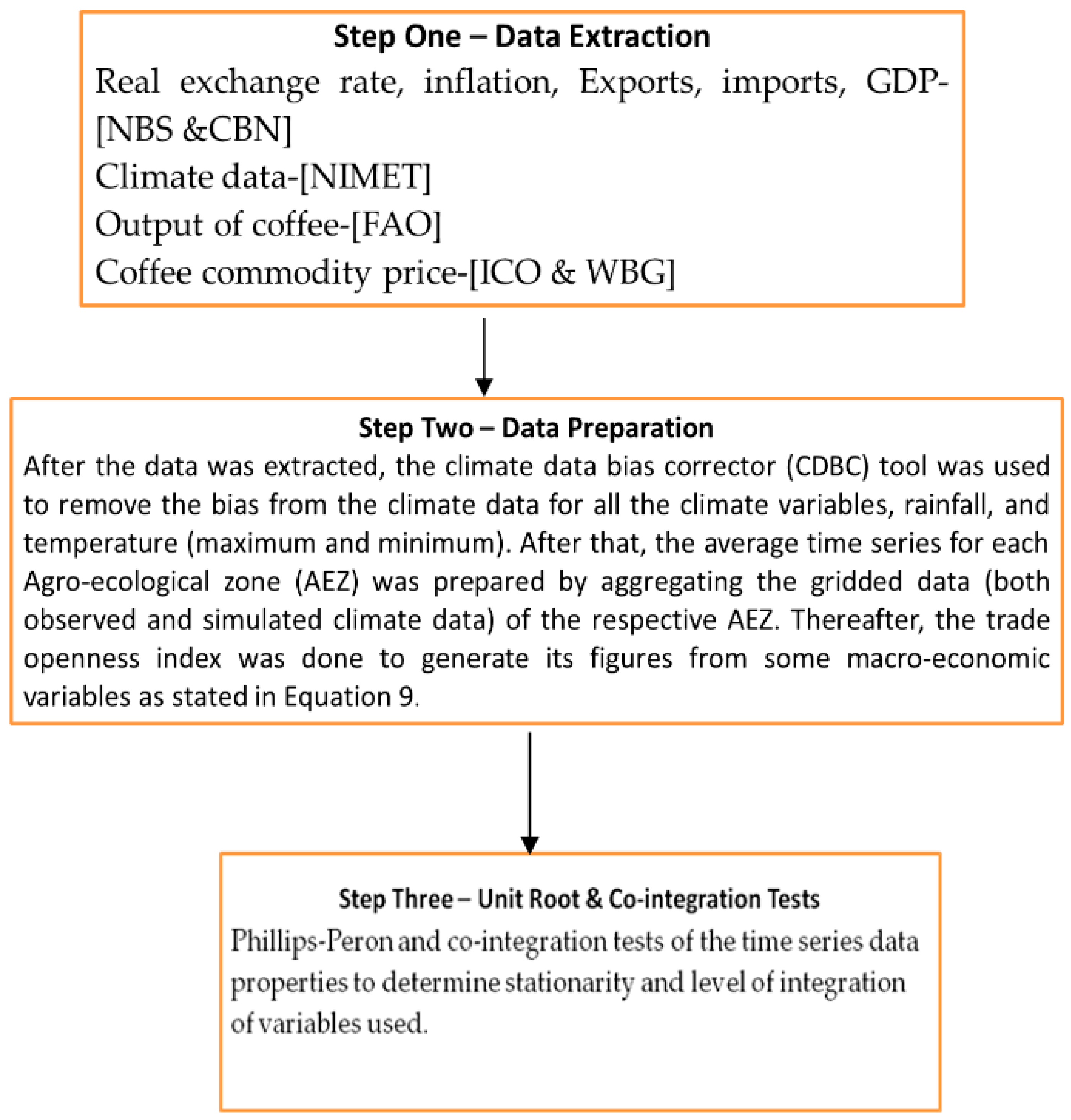
2.9. Pre-Data Processing Flow Chart

The secondary data used for the study was pre-processed before the analysis. The pre-Data processing flow chart is shown in Chart 1 below. This gives a very clear picture of the entire pre-data processing starting from the data extraction sources and variables sourced to Unit root and co-integration tests.

2.10. Similar Studies with Their Adopted Analytical Models

The adopted research analytical method by this study was compared with similar studies in the world. The summary of the adopted analytical methods with similar studies is shown in

Table 1. Summary of siamilar studies with their adopted analytical models.

Authors	Region	Period	Methods
[41]	Asian Countries	1980-2014	FMOLS
[42]	Pakistan	1988–2011	VAR, ARDL, and VECM
[43]	Pakistan	1980–2013	ARDL and VECM
[44]	14 MENA countries	1996–2012	FMOLS
[45]	Nigeria	1980–2008	ARDL and VECM
[46]	USA	1960–2010	VAR and ARDL
[47]	China	1975–2000	STIRPAT model
[48]	Tunisia	1971–2012	ARDL and ECM
[49]	Malaysia		VECM Model
[50]	China	1953–2006	ARDL
[51]	South Asia	1975–2011	Co-integration test and Granger causality test
[52]	Malaysia	1970–2008	Bounds test and Granger causality
[53]	China	1978–2006	STIRPAT model +
[54]	Turkey	1960–2007	F test
[55]	Turkey	1968–2005	VAR
[56]	Iran	1971–2007	ARDL
[57]	22 emerging countries	1990–2006	GMM
[58,59]	South Africa	1965–2008	ARDL
[60]	Indonesia	1975Q1–2011Q4	ARDL VECM IAA
[61]	13 European and 12 East Asia and Oceania countries	1989–2011	PVAR

STIRPAT, stochastic impacts by regression on population, affluence, and technology; GMM, generalized method of moments; URB, urbanization; EC, energy consumption; ARDL, autoregressive distributed lag model; VECM, vector error correction model; FD, financial development; SR, stock return; DCPS, domestic credit to private sector; EC, energy consumption; EG economic growth; POP population; CO₂, Carbon dioxide emission. Source: Adapted from [41] and improved.

. The Table 1 below displays the authors, the region studied, the period covered by the study and the methods adopted by the various studies.

3. Results and Discussions

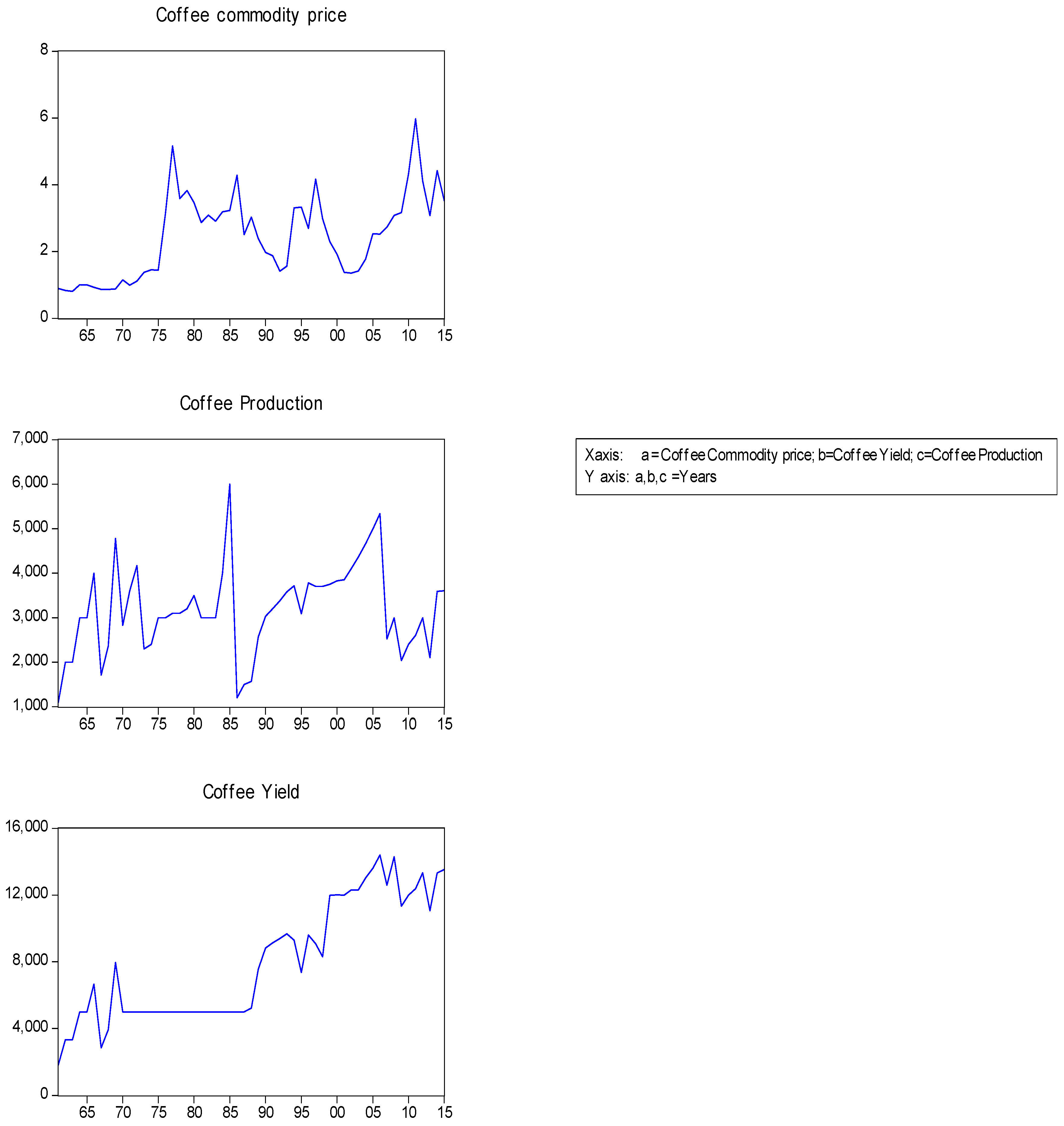
3.1. The Trend of Coffee Tree Crop Commodity Price, Production, and Yield 1961–2015

Considering the international monthly commodity prices of coffee tree crop for the 648 months (1961–2015), there has been considerable variability and instability of the prices of the commodity. As shown in Figure 1, the general trend pattern is characterized by sharp growth and also a sharp decline for the time period under study. Between 1961 and 1972, coffee recorded a somewhat similar pattern in its commodity price, which was accompanied immediately by a rapid growth from 1975 to 1978 followed by a sharp fall thereafter. It was also observed from Figure 1 that the upward trend did not characterize the whole period but rather a zigzag trend. In fact, there were steady fluctuations in commodity prices of the selected export tree crops from 1961 to 2015 as shown in Figure 1. Between 1975 and 1978 there was a sharp increase in coffee commodity price from below $2/kg to over $5/kg followed by a decline from 1978 and another sharp increase to its peak price of $5.98/kg recorded in 2011.

The graph of the trend of coffee tree crop yield (Tons/Ha) as also shown in Figure 1 reveals gradual fluctuations in coffee yield. Coffee yield trend was observed to show fluctuating trend but a steady yield value of 5000 Tons/ha was noticed from 1973 to 1983, and a gradual increase to 5233 Tons/ha from 1984 to 14,394 Tons/ha in 2006. The figure shows that the production of coffee showed a somewhat insignificant unstable trend of 4000 tons in 1966 to 6000 tons in 1985 and down to 3604 tons in 2015.

3.2. Determination of the Time Series Properties of Data Employed for Analysis

The properties of the time-series data used for the analysis were tested. Phillips-Peron [62] test (hereafter PP) was used in determining the stationarity of the variables under consideration and the results are presented in

Table 2. Unit root test result.

	Phillips-Perron Test
Variable	Level	1st Difference	Order of Integration
Climate change
Rainfall	−5.045133 (0.0001)		I(0)
Temperature	−4.260020 (0.0013)		I(0)
Commodity prices
Coffee	−2.565541 (0.1064)	−8.338275 (0.0000)	I(1)
Output (production)
Coffee	−5.406997 (0.0000)		I(0)
Output (Yield)
Coffee	−2.724048 (0.0766)		I(0)
Others
Real Exchange rate	1.310611 (0.9984)	−6.287971 (0.0000)	I(1)
Trade openness	−3.007864 (0.1396)	−9.084742 (0.0000)	I(1)
Inflation rate	−3.243140 (0.0228)		I(0)

Source: E-views 9 Researchers’ calculations output result from FAO, WBG, NBS, CBN, ICO, NIMET data. Note: Values in parentheses are probability values.

.

The PP test is a non-parametric test, but it was found to produce a superior result that corrects for serial correlation and heteroscedasticity. The PP test is also known to be better in the presence of regime shift, which is a problem usually encountered with macroeconomic data emanating from Africa [63]. On the application of PP, test variables attained stationarity at the level and also after differencing once and, thus, one may conclude that there is a mixed order of integration in the data. Stationarity is confirmed when the test statistic is greater that the critical value in absolute terms.

From Table 2, the entire test variables for examining coffee output (yield and production) reactions to climate change and commodity price volatility were stationary at the level and after first differencing for some on the basis of the PP probability tests. As such, one could reject the null hypothesis of non-stationarity. The occurrence of unit roots at a level in the price data generation process of the commodity gives a preliminary indication of shocks having a permanent or long-lasting effect, thus, not making it easy for traditional price stabilization policies common in African countries to survive [64].

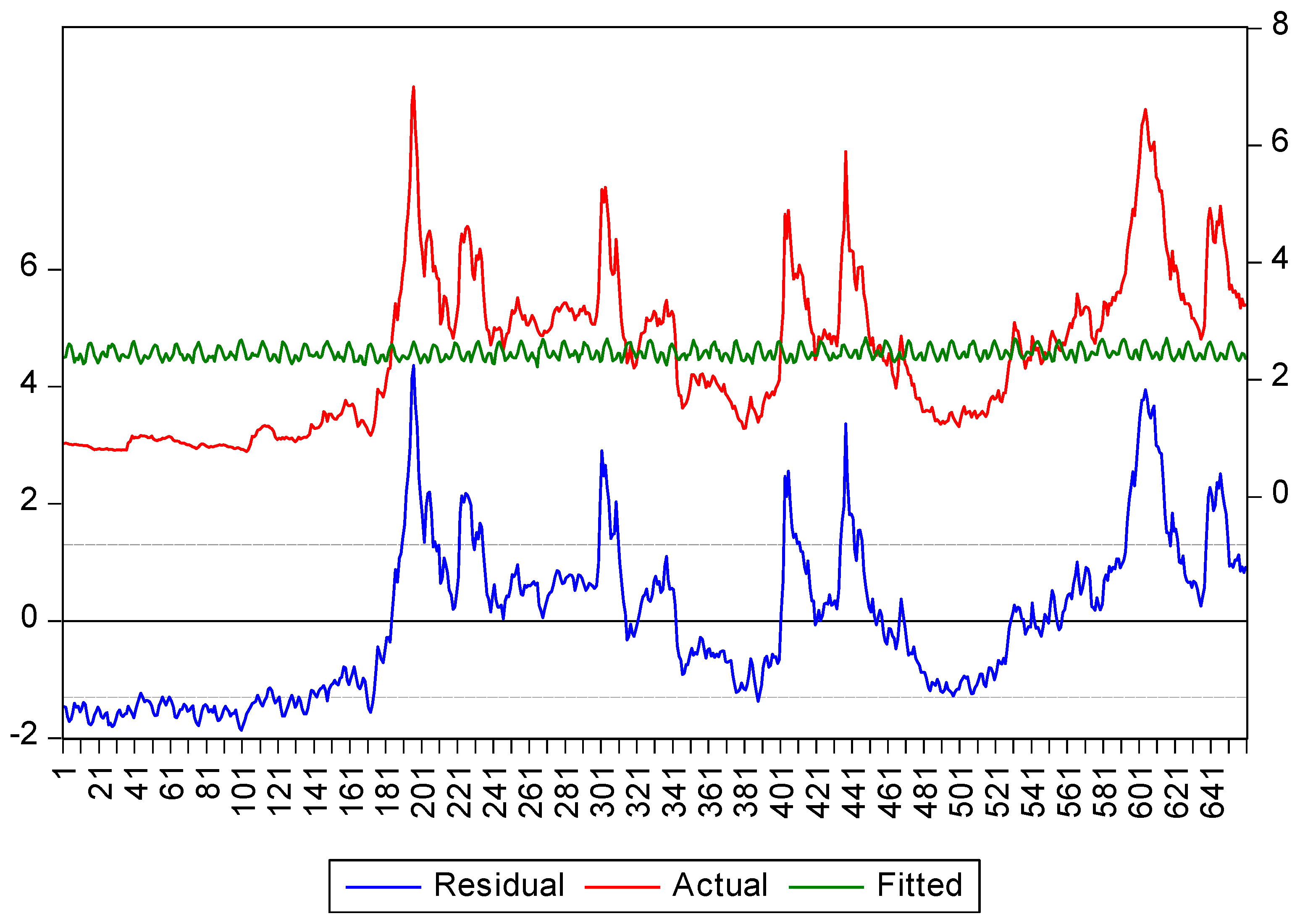
3.3. Volatility Test for Coffee Commodity Price

Results for the ARCH test for coffee commodity price are presented in

Table 3. Heteroscedasticity test of the residuals for coffee commodity price.

Heteroskedasticity Test: ARCH
F-statistic	4262.971	Prob. F(1,657)	0.0000
Obs*R-squared	570.9989	Prob. Chi-Square(1)	0.0000

Source: E-views 9 Researchers’ calculations output result from FAO, WBG, ICO data.

. The Engle’s LM test indicates that there are ARCH effects in coffee commodity price. The F-statistic value is significant at the 0.01 probability level and this implies that there is a presence of ARCH meaning that there is also the presence of heteroskedasticity in the residual.

The residual plot as shown in Figure 2 further strengthens and approves the strong presence of ARCH and serious heteroskedasticity in coffee commodity price.

Table 4. Volatility test for coffee commodity price.

GARCH = C(4) + C(5) × RESID(−1)2
Variable	Coefficient	Std. Error	z-Statistic	Prob.
Intercept	2.420292	0.226604	10.68073 ***	0.0000
Rainfall	−0.000204	0.000196	−1.041463	0.2977
Temperature	0.010139	0.008497	1.193291	0.2328
	Variance Equation
C	0.036791	0.006877	5.349758 ***	0.0000
RESID(−1)2	1.016783	0.120992	8.403714 ***	0.0000
R-squared	−0.025073	Mean dependent var		2.458062
Adjusted R-squared	−0.028193	S.D. dependent var		1.303766
S.E. of regression	1.322017	Akaike info criterion		2.611361
Sum squared resid	1148.258	Schwarz criterion		2.645394
Log-likelihood	−856.7493	Hannan-Quinncriteria.		2.624552
Durbin-Watson stat	0.030283

Source: Researchers’ calculations output result from Eviews version 9. ***, significant at the 0.01 probability level.

shows the results of the volatility test for coffee commodity price using the GARCH approach to verify the presence of volatility in coffee commodity within the period under study. The results show that coffee international commodity price is volatile. The coefficient of the lagged value of coffee commodity price (2.420) had a significant positive relationship with its current value (the dependent variable) overtime for the study period at 1% significant level. In the variance equation, the RESID(−1)² value of (1.016) confirmed the existence of volatility in coffee commodity price within the period under study.

The implication of the price volatility in coffee commodity price is that there could be the transmission of food price volatility from international to domestic markets. This is in line with the findings of [65].

3.4. Effects of Climatic Variations and Commodity Price Volatility on the Yield and Output of the Coffee Output

The parameter estimates of the cointegration regression model (fully modified ordinary least squares, FMOLS) applied in analyzing the climate variables alongside commodity price and combination of climate variables with commodity price of coffee tree crop to ascertain their effects on coffee output in Nigeria over the period of study are summarized in Table 4.

The test diagnosis statistics results in

Table 5. Results of fully modified ordinary least square (FMOLS) parameter estimates to model the effect of climate variables, commodity price volatility, and joint effect of climatic variables with commodity prices volatility on yield of coffee in Nigeria (1961–2015).

Dependent variable		Coffee Yield
Independent variables	Coefficient	Standard Error
Intercept	−59,997.33 (−2.486005)	24,134.030
Trend	129.0227 (5.134969) ***	25.126
Rainfall	−0.001484 (−0.617369)	0.002
Temperature	204.0113 (2.638827) *	77.311
Commodity price	28,474.40 (3.174368) ***	8970.099
Inflation	0.757708 (0.079467)	9.535
Trade openness	94.24276 (3.364582) ***	28.011
Real exchange rate	11.32584 (2.095428) **	5.405
Rainfall with commodity price	0.002371 (3.003671) ***	0.001
Temperature with commodity price	−95.73729 (−3.297216) ***	29.036
R-squared	0.94
Adjusted R-squared	0.92
Jarque Bera Statistic	0.100
Engle-Granger tau-statistic	−7.076 ***
Long Run Variance	698472.1
Remark on Correlogram of Residuals Squared	Not significant at 10%
Mean dependent var	8092.722

Source: Output result from Eviews version 9. Note: ***, ** and * = Figures significant at 1%, 5% and 10% probability levels.

showed that the test for model fitness gave an R² value of 0.94, implying that 94% of the variations in coffee yield were accounted for by variability in the independent variables included in the regression model. The model also had residuals, which were normally distributed with a Jarque Bera statistic of 0.100. Similarly, the cointegration test using Engle-Granger Tau statistic recorded a value of −7.076 (p < 0.01) whereby the null hypothesis held that “series are not cointegrated was rejected”. The series is, therefore, cointegrated and could be reliably used for forecasting.

It was observed further that temperature, coffee commodity price, trade openness, real exchange rate, and climate variables (rainfall and temperature respectively) with commodity price of coffee significantly influenced the yield of coffee in Nigeria at 10%, 5%, and 1% levels of significance, respectively. The slope coefficients of the mentioned variables included were 204.0113 (p < 0.10), 28474.0 (p < 0.01), 94.24276 (p < 0.01), 11.32584 (p < 0.05), 0.002371 (p < 0.01), and −95.73726 (p < 0.01). While it could be inferred from the results that climate variables combined with coffee commodity price together with trade openness and real exchange rate and coffee commodity price significantly determined the variability in yield of coffee over the period of study, temperature and precipitation changes more so do not exert the expected effect on coffee yields.

While temperature increase resulted in an increase of yield of coffee during the review period, it was observed that coffee yields, however, responded negatively to the increase in temperature combined with coffee commodity price in the study. A percentage increase in the volume of temperature resulted in an increase in coffee yield by 204.0113 tons; while a percentage rise in temperature combined with coffee commodity price resulted in a decrease in the yield of coffee by 95.73729 tons. The result is inconsistent with the findings of [44,66,67,68] who had positive and negative coefficients for temperature and rainfall on a similar study in Nigeria.

The caveat that can be deduced from these findings is that other parameters may be needed in explaining yield changes. Sometimes, climate change or variability can result in opportunities for an increase in yield or productivity of crops depending on the agronomic requirements of the particular crop under a particular, prevailing climate.

The indication from the result that showed that the combination of climate variable (temperature) with coffee commodity price exerted a negative significant influence on the yield of coffee in the study implies that an increase in value of combination of temperature with coffee commodity price was accompanied by a decrease in coffee yield by −95.73729 tons.

3.5. Effects of Climatic Variations, Commodity Prices Volatility, and Joint Effects of Climatic Variations with Commodity Prices Volatility on Coffee Production

In

Table 6. Results of FMOLS parameter estimates to model the effect of climate variables, commodity prices volatility, and joint effect of climatic variables with commodity prices volatility on production of coffee in Nigeria (1961–2015).

Dependent Variable			Coffee Production
Independent Variables	Coefficient	Standard Error	Coefficient	Standard Error
Intercept	−1,561,618 (−1.821641) *	857,259.1	−2905.669 (−2.419072) **	1201.150
Trend	274.5286 (0.341982)	802.757	0.038157 (2.813904) ***	0.014
Rainfall	−0.077223 (−0.959398)	0.081	6.27 × 10−6 (2.093096) **	3.00E-06
Temperature	5805.777 (2.128044) **	2728.222	−1.919630 (−2.466962) **	0.778
Commodity price	905,802.5 (2.133219) **	424617.6	−616.4039 (−2.446665) **	251.936
Inflation	434.9243 (1.320889)	329.266	0.002577 (0.054020)	0.048
Trade openness	2280.705 (2.349205) **	970.841	0.062987 (3.438604) ***	0.018
Real exchange rate	567.4082 (2.767124) ***	205.053	−0.331229 (−3.195231) ***	0.104
Rainfall with commodity price	0.175076 (4.080897) ***	0.043	−3.985003 (−1.589991)	2.506
Temperature with commodity price	−3328.699 (−2.426696) **	1371.7	620.0767 (2.456328) **	252.441
R-squared	0.36
Adjusted R-squared	0.21
Jarque Bera Statistic	6.014
Engle-Granger tau-statistic	−6.575 **
Long Run Variance	0.041624
Remark on Correlogram of Residuals Squared	Significant at 1%
Mean dependent var	8.046639

Source: Output result from Eviews version 9. Note: ***, ** and * = Figures significant at 1%, 5% and 10% probability levels.

, results of parameter estimates for the FM-OLS models used to analyze the effects of climate variables, commodity prices, and joint effects of climate variables with commodity prices on production of coffee tree crop in Nigeria from 1961 to 2015 are presented.

The model estimates’ diagnosis of the residuals done for coffee production indicated that the series was cointegrated with Engle–Granger Tau statistics of −6.575 (p > 0.06) implying that a long-run stable relationship does not exist among the series. The model’s residuals also exhibited a Jarque Bera statistics of 6.014, implying that the residuals were normally distributed. With the estimated correlogram of the residuals squared significant at 1%, it can be concluded that the residuals were not fraught with serious threats of neither serial correlation nor severe multicollinearity in the model. The model also showed a good fit for the R² level and, thus, implies a good fitting of the model.

As can be observed in Table 6, coffee production was significantly determined by six variables that included rainfall (6.27 × 10⁻⁶; p < 0.06), temperature (−1.919630; p < 0.06), coffee commodity price (−616.4039, p < 0.05), trade openness (0.062987; p < 0.02), and temperature with coffee commodity price (620.0767, p < 0.05). The recorded significant effect of rainfall and combination of temperature with coffee commodity price implied that climate variability is an important factor influencing the production of coffee in Nigeria. It was specifically observed that a percentage increase of rainfall during the period in review resulted in a production increase of coffee by 6.27 tons while a percentage increase of the combination of temperature with coffee commodity during the period in review resulted in a production increase of coffee by 620.0767 tons. This result demonstrates the influence of climate variables on farmers’ decision to produce coffee, showing that weather is important in determining the production of coffee in the country.

Amongst the six significant variables, rainfall, trade openness, and the combination of temperature with coffee commodity price posed as positive significant determinants of production of coffee in Nigeria over the period of study. The effect implies that rainfall, trade openness, and the combination of temperature with coffee commodity are huge determinant factors in coffee production and export. For instance, the slope coefficient of rainfall, trade openness, and the combination of temperature with the coffee commodity in the study showed that a percentage increase in rainfall, trade openness, and the combination of temperature with coffee commodity resulted in an increase in production of coffee by about 6.27, 0.062987, and 620.0767 tons, respectively.

As for temperature, coffee commodity price, and real exchange rate, it was found that their significant effects on the production of coffee were negative. It was specifically found that a percentage change in their values resulted in a decrease in coffee production by 1.919630, 616.4039, and 0.331229 tons, respectively in the economy during the period in review. This finding is similar to the findings of [50] but disagrees with the findings of [46,48,54,55].

3.6. Test of Hypotheses

In

Table 7. Pairwise Granger causality tests.

Null Hypothesis:	Obs	F-Statistic	Prob.
The coffee output does not Granger Cause Rainfall	53	0.22433	0.7999
Rainfall does not Granger Cause coffee output		0.19904	0.8202
The coffee output does not Granger Cause Temperature	53	3.05113 *	0.0566
Temperature does not Granger Cause coffee output		1.06039	0.3543
Temperature does not Granger Cause D(coffee commodity price)	52	0.04543	0.9556
D(commodity price) does not Granger Cause Temperature		0.38295	0.6840

Note: * = Figures significant at 10% probability levels.

, the results of pairwise Granger causality test on the relationship between coffee tree crop output, climate change variables, and coffee commodity price are presented.

Hypothesis 1.

There is no significant relationship between the output of selected coffee tree crop and the variation of rainfall in Nigeria.

The null hypothesis that held that rainfall did not Granger cause coffee output and vice versa were accepted as their F-Statistic were not significant at any probability level. This enabled us to conclude that rainfall has no significant relationship with the output of coffee and vice versa.

Hypothesis 2.

Variation in temperature has no significant effect on coffee tree crop output in Nigeria.

In testing hypothesis two, the null hypothesis that coffee output did not Granger cause temperature gave an F-Statistic of 3.05113 (p > 0.05) indicating that we have to reject the hypothesis at a significant value of 10%. This enabled us to conclude that coffee output influenced the variation of temperature.

It would, thus, be interpreted that the outputs of coffee in the previous year will transmit information to its producers, marketers, or exporters that there would be either glut or scarcity of the product in the present year as its output is associated with variation of temperature degrees. This will, in turn, influence the present international commodity prices of these tree crops.

Hypothesis 3.

Commodity price volatility has no significant effect on coffee tree crop output in Nigeria.

The null hypotheses that held that the international commodity prices of coffee did not Granger cause coffee output and vice versa were accepted as their F-Statistic were not significant at any probability level. This enabled us to conclude that the commodity price of coffee tree crop has no significant effects on the outputs of coffee and vice versa.

3.7. Summary of Findings

The study examined the response of climate variability, commodity prices volatility, and other select macro-economic indicators on the output of coffee tree crop in Nigeria 1961–2015. Descriptive statistics, GARCH, and ARCH models and the F-MOLS were analytical tools employed to realize the specific objectives.

The descriptive analysis of the trend in commodity prices, yield, and production of coffee export tree crop showed there are fluctuations (upward and downward trend) in price, yield, and production of the coffee tree crop.

In determining the time series properties of data employed, the results of the unit root test by Philip-Perron showed a mixed order of integration among the variables employed. That is to say that, some of the variables were nonstationary in their level form but became stationary when subjected to the first difference.

The result from the volatility test shows that there is volatility in the international commodity price of coffee. The coefficient of the lagged value of their commodity price had a significant positive relationship with its current value over time for the study period. The variance equation value of coffee tree crops still confirmed the existence of volatility in their commodity prices within the period under study.

The analysis on the effects of climate variables, commodity price, and combination of climate variables with commodity price to ascertain their effects on coffee tree crops yield using FM-OLS showed that the model used had a good fit with their observed R² levels and other diagnosis statistics.

Specifically, the yield of coffee showed that it was negatively affected by a combination of climate variable (temperature) with coffee commodity price at 1% level of significance and positively affected by temperature, coffee commodity price, trade openness, real exchange rate, and combination of rainfall with coffee commodity at 10%, 1%, and 5% levels of significance, respectively.

Furthermore, coffee production result from the FM-OLS showed that it was positively influenced by rainfall, trade openness, and combination of temperature with coffee commodity price at different levels of significance, respectively, and negatively by temperature, coffee commodity price, and real exchange rate, also at various levels of significance.

More so, the null hypothesis that held that rainfall did not Granger cause coffee output and vice versa were accepted while, the null hypothesis that coffee output did not Granger cause temperature was rejected. Also, the null hypotheses that held that the international commodity prices of coffee did not Granger cause coffee output and vice versa and the null hypothesis that held that coffee output did not Granger cause coffee commodity price were accepted. However, the null hypothesis that held that coffee output did not Granger cause temperature was rejected.

4. Conclusions

Based on the findings of this study, the conclusion, therefore, is that there is a need for trade facilitation to reduce inherent risks in agribusiness marketing by re-introducing and re-invigorating the Centre for Agricultural Commodity Marketing (CACMART) by the Government of Nigeria through its institutions.

References

1. World Bank Group. Agribusiness and Value Chains. Understanding Poverty Report Updated. Available online: https://www.worldbank.org/en/topic/agribusiness (accessed on 24 September 2018).
2. African Development Bank (AfDB). Level 1 Development in Africa. In Annual Development Effectiveness Review; AfDB: Abidjan, Côte d’Ivoire, 2015. [Google Scholar]
3. World Bank Group. World Bank Report on the Potential of Agribusiness in Africa 2018. Available online: http://www.worldbank.org/en/news/feature/2013/03/04/africa-agribusiness-report (accessed on 15 March 2019).
4. Akinbobola, T.O.; Adedokun, S.A.; Nwosa, P.I. The Impact of Climate Change on Composition of Agricultural Output in Nigeria. Am. J. Environ. Prot. 2015, 3, 44–47. Available online: http://pubs.sciepub.com/env/3/2/1/env-3-2-1.pdf (accessed on 7 September 2016). [CrossRef]
5. International Coffee Organization (ICO). World Coffee Production Report. 2019. Available online: http://www.ico.org/prices/po-production.pdf (accessed on 15 March 2019).
6. Petchers, S.; Harris, S. The roots of the coffee crisis. In Confronting the Coffee Crisis: Fair Trade Sustainable Livelihoods and Ecosystems in Mexico and Central America; Bacon, C.M., Méndez, V.E., Gliessman, S.R., Goodman, D., Fox, J.A., Eds.; MIT Press: Cambridge, MA, USA, 2008; pp. 43–66. [Google Scholar]
7. International Coffee Organization (ICO). Volatility of Prices Paid to Coffee Growers in Selected Exporting Countries; ICO Document; ICC: London, UK, 2011; pp. 107–110. [Google Scholar]
8. International Coffee Council (ICC). Impact of the Coffee Crisis on Poverty in Producing Countries; 89th Session; ICC: Cartagena, Colombia, 2003; pp. 89–95, Rev. 1. [Google Scholar]
9. Ortiz-Miranda Dionisio, A.; Moragues-Faus, M. Governing Fair Trade Coffee Supply: Dynamics and Challenges in Small Farmers’ Organizations. Sustain. Dev. 2015, 23, 41–54. [Google Scholar] [CrossRef]
10. Food and Agriculture Organization (FAO). The State of Food Insecurity in the World 2011, Policy Options to Address Price Volatility and High Prices. Available online: http://www.fao.org/docrep/014/i2330e/i2330e05.pdf (accessed on 7 September 2016).
11. African Development Bank (AfDB). AfDB Gender Strategy (2014–2018); AfDB: Tunis, Tunisia, 2014. [Google Scholar]
12. Ayodeji, A.; Ajibola, C.; Oladipo Akogun, E.; Owoniyi Adebayo, C.; Shaba, M.; Mercy, N.; Halimat, S.; Hamdalat Opeyemi, J. Gender Differentials among Subsistence Rice Farmers and Willingness to undertake Agribusiness in Africa: Evidence and Issues from Nigeria. Afr. Dev. Rev. 2017, 29, 198–212, No. S2. [Google Scholar]
13. Federal Office of Statistics (FOS). Geography of Federal Republic of Nigeria; FOS: Malaysia, Vietnam, 1989. [Google Scholar]
14. World Bank. Project Appraisal Document on a Proposed Credit for Transforming Irrigation Management in Nigeria Project; World Bank: Washington, DC, USA, 2014. [Google Scholar]
15. Food and Agriculture Organization (FAO). How to Feed the World in 2050, High Level Expert Forum-Office of the Director, Agricultural Development Economics Division Economic and Social Development Department Viale delle Terme di Caracalla, 00153 Rome, Italy. 2009. Available online: http://www.fao.org/fileadmin/templates/wsfs/docs/Issues_papers/HLEF2050_Investment.pdf (accessed on 7 September 2016).
16. National Bureau of Statistics (NBS). National Bureau of Statistics Report on Nigerian Population Estimate as at 2013. Available online: http://www.nigerianstat.gov.ng/pdfuploads/2014%20Statistical%20Report%20on%20Women%20and%20Men%20in%20Nigeria_.pdf (accessed on September 2016).
17. Nigerian Meteorological Agency (NIMET). Nigerian Meteorol Agency Report; NIMET: Kaduna, Nigeria, 2008. [Google Scholar]
18. Phillips, S.J.; Anderson, R.P.; Schapire, R.E. Maximum entropy modeling of species geographic distributions. Ecol. Model. 2006, 190, 231–259. [Google Scholar] [CrossRef] [Green Version]
19. Schroth, G.; Laderach, P.; Dempewolf, J.; Philpott, S.M.; Haggar, J.P.; Eakin, H.; Castillejos, T.; Garcia-Moreno, J.; Soto-Pinto, L.; Hernandez, R.; et al. Towards a climate change adaptation strategy for coffee communities and ecosystems in the Sierra Madre de Chiapas, Mexico. Mitig. Adapt. Strateg. Glob. Chang. 2009, 14, 605–625. [Google Scholar] [CrossRef] [Green Version]
20. Rahn, E.; Laderach, P.; Baca, M.; Cressy, C.; Schroth, G.; Malin, D.; van Rikxoort, H.; Shriver, J. Climate change adaptation and mitigation in coffee production: Where are the synergies? Mitig. Adapt. Strateg Glob. Chang. 2014. [Google Scholar] [CrossRef]
21. Laderach, P.; van Asten, P. Coffee and climate change. Coffee suitability in East Africa. In Proceedings of the 9th African Fine Coffee Conference and Exhibition, Addis Ababa, Ethiopia, 16–18 February 2012. [Google Scholar]
22. Laderach, P.; Martinez, A.; Schroth, G.; Castro, N. Predicting the future climatic suitability for cocoa farming of the world’s leading producer countries, Ghana and Côte d’Ivoire. Clim. Chang. 2013, 119, 841–854. [Google Scholar] [CrossRef]
23. Guardian. Much ado about Nigeria’s Dwindling Coffee Cultivation Level. Guardian Newspapers. 2019. Features Report By Gbenga Akinfenwa on 06 January 2019. Available online: https://guardian.ng/features/agro-care/much-ado-about-nigerias-dwindling-coffee-cultivation-level/ (accessed on 15 March 2019).
24. Hijmans, R.J.; Cameron, S.E.; Parra, J.L.; Jones, P.G.; Jarvis, A. Very high resolution interpolated climate surfaces for global land areas. Int. J. Climatol. 2005, 25, 1965–1978. [Google Scholar] [CrossRef]
25. Lobo, J.M.; Tognelli, M.F. Exploring the effects of quantity and location of pseudo-absences and sampling biases on the performance of distribution models with limited point occurrence data. J. Nat. Conserv. 2011, 19, 1–7. [Google Scholar] [CrossRef]
26. Barbet-Massin, M.; Jiguet, F.; Albert, C.H.; Thuiller, W. Selecting pseudo-absences for species distribution models: How, where and how many? Methods Ecol. Evol. 2012, 3, 327–338. [Google Scholar] [CrossRef]
27. Schroth, G.; Läderach, P.; Blackburn, D.S.B.; Neilson, J.; Bunn, C. Winner or loser of climate change? A modeling study of current and future climatic suitability of Arabica coffee in Indonesia. Reg. Environ. Chang. 2015, 15, 1473–1482. [Google Scholar] [CrossRef]
28. Liu, C.; White, M.; Newell, G. Selecting thresholds for the prediction of species occurrence with presence-only data. J. Biogeogr. 2013, 40, 778–789. [Google Scholar] [CrossRef]
29. Kenen, P.B.; Rodrik, D. Measuring and Analysing the Effects of Short-term Volatility in Real Exchange Rate. Rev. Econ. Stat. 1986, 68, 311–315. [Google Scholar] [CrossRef]
30. Bailey, M.; George, T.; Micheal, U. Exchange Rate Variability and Trade Performance: Evidence for the Big Seven Industrial Countries. Weltwirlschaftliches Archiv. 1986, 1, 467–477. [Google Scholar] [CrossRef]
31. Peree, E.; Steineir, A. Exchange Rate Uncertainty and Foreign Trade. Eur. Econ. Rev. 1989, 33, 1241–1264. [Google Scholar] [CrossRef]
32. Côté, A. Exchange Rate Volatility and Trade: A Survey. In Bank of Canada. Working Paper; Bank of Canada: Ottawa, ON, Canada, 1994; pp. 94–95. Available online: https://www.bankofcanada.ca/wp-content/uploads/2010/04/wp94-5.pdf (accessed on 15 March 2019).
33. McKenzie, M.; Brooks, R.D. The impact of ERV on German-U.S Trade Flows. J. Int. Financ. Mark. Inst. Money 1997, 7, 73–87. [Google Scholar] [CrossRef]
34. Engle, R.F. Autoregressive Conditional Heteroscedasticity with Estimates of the Variance of UK Inflation. Econometrica 1982, 50, 987–1008. [Google Scholar] [CrossRef]
35. Bollerslev, T. Generalized Autoregressive Conditional Heteroscedasticity. J. Econom. 1986, 6, 307–327. [Google Scholar] [CrossRef]
36. Yinusa, D.O. Between dollarization and Exchange Rate Volatility: Nigeria’s Portfolio Diversification Option. J. Policy Model. 2008, 30, 811–826. [Google Scholar] [CrossRef]
37. Akpokodje, G. Exchange rate volatility and External Trade: The Experience of Selected African Countries. In Applied Econometrics and Macroeconomic Modelling in Nigeria; Adeola, A., Dipo, B., Olofin, S., Eds.; Ibadan University Press: Ibadan, Nigerija, 2009; pp. 79–87. [Google Scholar]
38. Olowe, R.A. Modelling Naira/Dollar Exchange Rate Volatility: Application of GARCH and Assymetric Models. Int. Rev. Bus. Res. Pap. 2009, 5, 377–398. [Google Scholar]
39. Phillips, P.C.B.; Hansen, B.E. Statistical inference in instrumental variables regression with I (1) processes. Rev. Econ. Stud. 1990, 57, 99–125. [Google Scholar] [CrossRef]
40. Granger, C.W.J. Investigating Causal Relations by Econometric Models and Cross-Spectral Methods. Econometrica 1969, 37, 424–438. [Google Scholar] [CrossRef]
41. Philips, P.C.B.; Perron, P. Testing for a unit root in time series regression. Biometrika 1988, 73, 335–346. [Google Scholar] [CrossRef]
42. Abdul, Q.K.; Naima, S.; Syeda, T.F. Financial development, income inequality, and CO2 emissions in Asian countries using STIRPAT model. Environ. Sci. Pollut. Res. 2018, 25, 6308–6319. [Google Scholar] [CrossRef]
43. Abbasi, F.; Riaz, K. CO2 emissions and financial development in an emerging economy: An augmented VAR approach. Energy Policy 2016, 90, 102–114. [Google Scholar] [CrossRef]
44. Ahmed, K.; Shahbaz, M.; Qasim, A.; Long, W. The linkages between deforestation, energy and growth for environmental degradation in Pakistan. Ecol. Indic. 2015, 49, 95–103. [Google Scholar] [CrossRef]
45. Al-Mulali, U.; Ozturk, I. The effect of energy consumption, urbanization, trade openness, industrial output, and the political stability on the environmental degradation in the MENA (Middle East and North African) region. Energy 2015, 84, 382–389. [Google Scholar] [CrossRef]
46. Bello, A.K.; Abimbola, O.M. Does the level of economic growth influence environmentalquality in Nigeria: A test of environmental Kuznets curve (EKC) hypothesis. Pak. J. Soc. Sci. 2010, 7, 325–329. [Google Scholar]
47. Dogan, E.; Turkekul, B. CO2 emissions, real output, energy consumption, trade, urbanization and financial development: Testing the EKC hypothesis for the USA. Environ. Sci. Pollut. Res. 2016, 23, 1203–1213. [Google Scholar] [CrossRef]
48. Fan, Y.; Liu, L.C.; Wu, G.; Wei, Y.M. Analyzing impact factors of CO2 emissions using STIRPAT model. Environ. Impact Assess. Rev. 2006, 26, 377–395. [Google Scholar] [CrossRef]
49. Farhani, S.; Ozturk, I. Causal relationship between CO2 emissions, real GDP, energy consumption, financial development, trade openness, and urbanization in Tunisia. Environ. Sci. Pollut. Res. 2015, 22, 15663–15676. [Google Scholar] [CrossRef] [PubMed]
50. Islam, F.; Shahbaz, M.; Alam, M. Financial development and energy consumption nexus in Malaysia: A multivariate time series analysis. In MPRA Paper 28403; University Library of Munich: Munch, Germany, 2011. [Google Scholar]
51. Jalil, A.; Feridun, M. The impact of growth, energy and financial development on the environment in China: A cointegration analysis. Energy Econ. 2011, 33, 284–291. [Google Scholar] [CrossRef]
52. Azam, M.; Khan, A.Q.; Bakhtyar, B.; Emirullah, C. The causal relationship between energy consumption and economic growth in the ASEAN-5 countries. Renew. Sustain. Energy Rev. 2015, 47, 732–745. [Google Scholar] [CrossRef]
53. Lau, L.S.; Choong, C.; Eng, Y.K. Investigation of the environmental Kuznets curve for carbon emissions in Malaysia: Do foreign direct investment and trade matter? Energy Policy 2014, 68, 490–497. [Google Scholar] [CrossRef]
54. Lin, S.; Zhao, D.; Marinova, D. Environmental impact of China: Analysis based on the STIRPAT model. In Proceedings of the Second International Association for Energy Economics (IAEE) Asian Conference, Perth, Australia, 5–7 November 2008; Cabalu, H., Marinova, D., Eds.; Curtin University of Technology: Perth, Australia, 2008; pp. 164–192. [Google Scholar]
55. Ozturk, I.; Acaravci, A. The long-run and causal analysis of energy, growth, openness and financial development on carbon emissions in Turkey. Energy Econ. 2013, 36, 262–267. [Google Scholar] [CrossRef]
56. Acaravci, A.; Ozturk, I. On the relationship between energy consumption, CO2 emissions and economic growth in Europe. Energy 2010, 35, 5412–5420. [Google Scholar] [CrossRef]
57. Saboori, B.; Soleymani, A. CO2 emissions, economic growth and energy consumption in Iran: A cointegration approach. Int. J. Environ. Sci. 2011, 2, 44–53. [Google Scholar]
58. Sadorsky, P. The impact of financial development on energy consumption in emerging economies. Energy Policy 2010, 38, 2528–2535. [Google Scholar] [CrossRef]
59. Shahbaz, M.; Mutascu, M.; Azim, P. Environmental Kuznets curve in Romania and the role of energy consumption. Renew. Sustain. Energy Rev. 2013, 18, 165–173. [Google Scholar] [CrossRef] [Green Version]
60. Hahbazm, O.I.; Afza, T.; Ali, A. Revisiting the environmental Kuznets curve in a global economy. Renew. Sustain. Energy Rev. 2013, 25, 494–502. [Google Scholar] [Green Version]
61. Shahbaz, M.; Hye, Q.; Tiwari, A.K.; Leitão, N.C. Economic growth, energy consumption, financial development, international trade and CO2 emissions in Indonesia. Renew. Sustain. Energy Rev. 2013, 25, 109–121. [Google Scholar] [CrossRef]
62. Ziaei, S.M. Effects of financial development indicators on energy consumption and CO2 emission of European, East Asian and Oceania countries. Renew. Sustain. Energy Rev. 2015, 42, 752–759. [Google Scholar] [CrossRef]
63. Yusuf, S.A.; Yusuf, W.A. Determinants of selected agricultural export crops in Nigeria: An ECM approach. In Proceedings of the African Association of Agricultural Economists, Abuja Nigeria, 23–26 September 2007; pp. 469–472. [Google Scholar]
64. Cashin, P.; Céspedes, L.; Sahay, R. Commodity Currencies and the Real Exchange Rate. J. Dev. Econ. 2004, 75, 239–268. [Google Scholar] [CrossRef]
65. Musunuru, N. Testing the presence of calendar anomalies in agricultural commodity markets. Reg. Bus. Rev. 2013, 32, 32–47. [Google Scholar]
66. Kalu, C. Impact of Climate Variability and Change on Supply of Grain in Nigeria from 1961–2012. Unpublished Ph.D. Dissertation, Department of Agribusiness and Management, Michael Okpara University of Agriculture, Umudike, Abia State, Nigeria, 2015; pp. 28–45. [Google Scholar]
67. Lloyd, T.A.; McCorriston, S.; Morgan, C.W.; Zgovu, E. The Experience of Food Price Inflation across the EU. In TRANSFOP; Working Paper No.5, TRANSFOP Project, EU 7th Framework Programme, Grant Agreement No. KBBE-265601-4-TRANSFOP; 2014; Available online: http://www.transfop.eu/ (accessed on 7 September 2016).
68. Ayinde, O.E.; Ojehomon, V.E.T.; Daramola, F.S.; Falaki, A.A. Evaluation of the effects of climate change on rice production in Niger State, Nigeria. Ethiop. J. Environ. Stud. Manag. 2013, 6, 763–773. [Google Scholar] [CrossRef]
Chart 1. A flow chart of data pre-process by authors.
Sustainability 11 03503 ch001
Figure 1. Trend of coffee tree crop commodity price, production, and yield 1961–2015.
Sustainability 11 03503 g001
Figure 2. Residuals plot for coffee commodity price. Source: Researchers’ calculations output result from Eviews version 9.
Sustainability 11 03503 g002