1. Introduction
As a cosmic industry, tourism delivers a variety of auxiliary services. The tourism industry of South Korea plays a vital role toward boosting the national economy; especially in the past few years, it has had an accelerated impact. According to a report, the contribution of tourism toward the country’s total gross domestic product (GDP), employment, and investments in 2017 was recorded to be 1.6% of the total GDP, 5.3% of total employment, and 2.3% of total investments, respectively, and these contributions are expected to rise by 3.5% for GDP, 1.8% for employment, and 2.4% for investments by 2028 [
1].
The tourist experience has dramatically changed in recent years with the huge boost in the tourism industry. In the tourism industry, sustainability can be mainly of two types. One is for the sustainable tourists’ experience, and other is for the sustainable destination environment. In this paper, our focus is on the sustainability of the tourists’ experience so that the tourists get the most satisfactory, enjoyable, and on-demand travel experience, according to the variable conditions of the destination. A pleasing tour is one where the involved factors and risks are manageable. A tour typically consists of four main factors: conveyance, sightseeing, accommodation, and food. The conveyance and sightseeing are inter-related, and can be combined to form one problem of first selecting the tourist attraction and then finding a route for conveyance to the selected spot. Although it sounds like a simple two-fold problem, it has many variable parameters involved in it that need to be taken care of in order to ensure a sustainable tourist’s experience. The involved variables in tourism change with the change in location, such as the road conditions, weather conditions, tourist’s in-flow rate at the destination, etc. Hence, an invulnerable system is required for the tourists’ sightseeing recommendation and route optimization to the site based on the current ground conditions of the location from source to destination. Such a system can not only provide an upgraded tourists experience in the average scenarios, but can also ensure a better balanced experience for the tourists in the possible worst case scenarios.
Forecasting the destination or next most probable route to be taken by the driver is valuable for several purposes. One of the primary purposes can be assisting the driver with a personalized driving experience by providing functions as alerts, risk calculation and extenuation, alternative routes based on traffic congestion, or any other unforeseen circumstances. Besides that, for hybrid vehicles, having the knowledge of routes beforehand serves to optimize the schedule of fuel charging, which in some cases have shown enhancements of up to 7.8% in fuel economy [
2]. As far as the driver’s significant intents are concerned, route and destination prediction have been the subject of numerous efforts by the research community [
3,
4,
5,
6,
7]. There are many applications that make use of route prediction in order to assist the drivers in multiple ways. Drivers these days mostly use navigation applications to get better routes for their trips.
Mostly, the observed routine in our driving is that we tend to visit the same destinations again and again, typically resulting in the selection of the same routes probably at the same time or day. Route selection is mostly based on the history of the driver’s driving habits; although they have much efficient and shorter alternatives, drivers tend to follow the routes that they have used in past. According to research, 60% of the routes are recurring and can be predictable based on the driving history [
6]. Another study suggests that more than 90% of the routes or paths that a user selects are possibly predictable based on the patterns of user mobility [
8]. Many approaches and models have been proposed. Some used global positioning satellite (GPS) data [
6] to discover the geometric similarity among trajectories; other approaches focused on Markov chains and hidden Markov models in order to extract the expected routes and destinations, including the most likely turns to be taken by the driver or tour clusters, etc. [
3,
9,
10]. These approaches were developed upon the roads’ network structure.
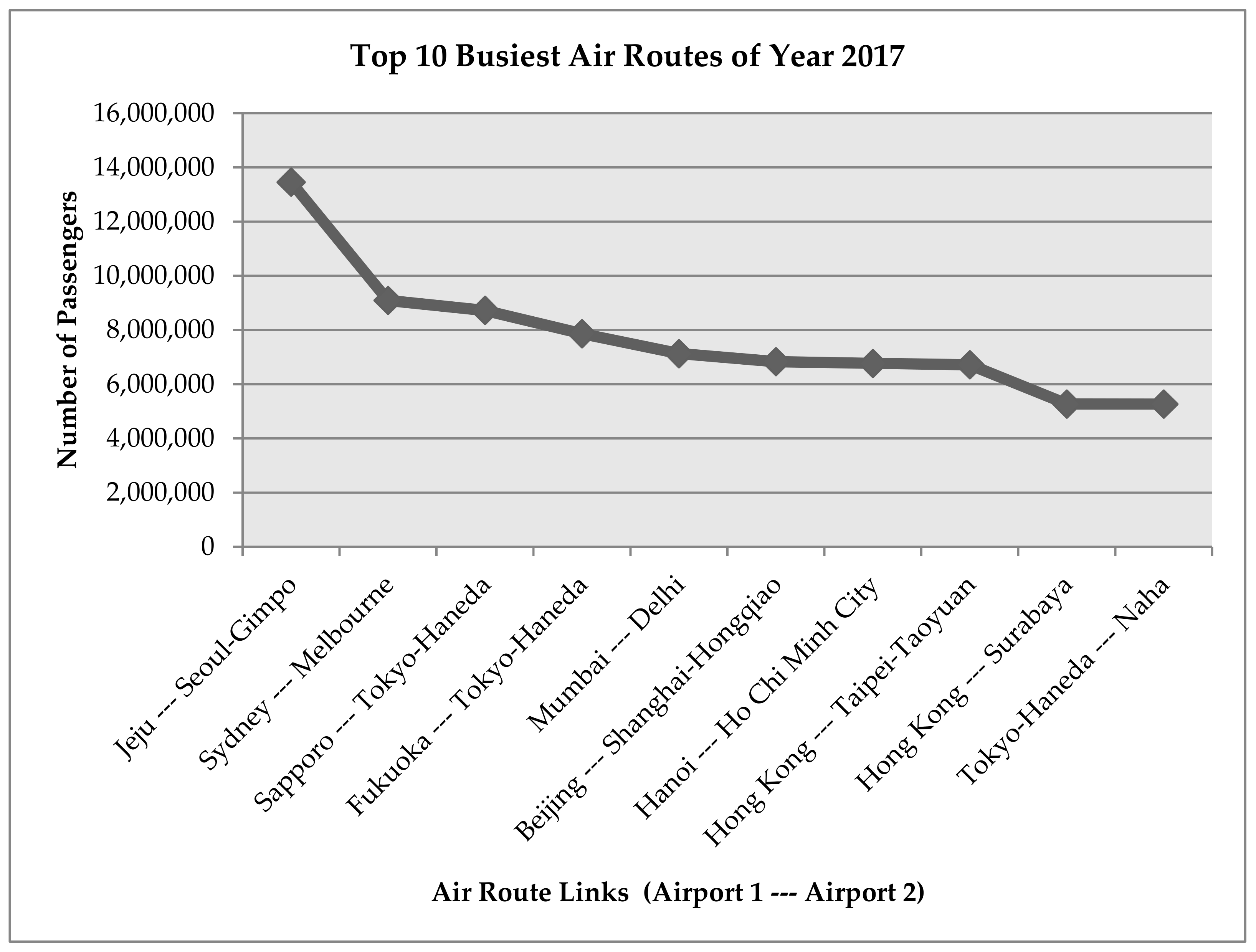
In this work, we use the tourism data of Jeju Island (South Korea) for optimal travel route recommendation to a selected tourist site. Jeju Island is a self-governing province that is known for its beach resorts and volcanic landscape. Jeju is a prime tourism destination for both domestic and international tourists as a vital region contributing significantly toward the country’s economy. Jeju is blessed with different resources and places that attract tourists from all over the world [
11]. The primary air route to Jeju is the domestic link between Gimpo airport (Seoul) and Jeju airport, which was listed as the world’s busiest air route for the year 2017, with a total number of 13,460,306 passengers (
Figure 1) [
12].
Therefore, considering the high interest of tourists in Jeju Island, the tourist data of Jeju Island is being used in this study. The swift information dispersion, rapid advancements in communication technologies, and unremitting flow of information have resulted in the dire need for continuous advancements and improvements in the facilities or services provided to tourists in order to deliver them ease and satisfaction. Optimal route identification and recommendation is one of these amenities, which requires our attention as a basic and much-needed facility to improve the traveler experience.
In this paper, one of the primary focuses is to provide an optimal route recommendation to the next point that a tourist will visit during his or her tour, which is predicted based on the previously visited and current location. We predict the most probable next location by using neural networks for learning the patterns with the impact of different input parameters as past routes, season, day, time, and vehicles on the route. The route optimization is performed using particle swarm optimization (PSO) for finding the optimal route to the next location.
The rest of the paper is structured as follows. In
Section 2, we present the literature review. In
Section 3, we present the proposed methodology for the route recommendation model. In
Section 4, we present the data set and experimental setup.
Section 5 contains the results analysis. In
Section 6, we present the comparative analysis with some related works, and
Section 7 concludes the paper.
2. Related Work
In recent years, route prediction has become a hot research topic, and many research methods have been proposed. A probabilistic forecast-based novel algorithm for the prediction of a tourist’s destination is presented in [
13]. The proposed algorithm works on probabilities; i.e., for every possible destination, it predicts a complete route plan toward that destination. The probabilities are accumulated on all the roads along the planned route for their respective destinations; high probabilities are assigned to roads leading toward or alongside the higher probability destinations. The algorithm learns a parameter, and once it’s calculated, there remains no need to store the tour history, and it can perform accurate predictions for the places where a tourist has never been before. The evaluations were performed for 100 recorded routes with the help of GPS.
For any tourist or traveler, planning a beautiful yet easy and efficient route toward his or her destination can be considered one of the primary tasks. Therefore, for automated route prediction applications or services, it is necessary to identify the essential elements and attributes of the route linked with the external environment, e.g., its scenery. To achieve this purpose of attributes identification, a model named path-size logit (PSL), which is also known as the route selection model, is presented in [
14]. Based on different volunteered geographical data for California as the study area, a set of scenic routes is formulated. The evaluations are performed against three PSL models.
Apart from the attributes of the route for destination planning, route recommendations, and advertising the tourist attractions, understanding the traveler’s mobility patterns plays an essential part. The work presented by Zheng et al. [
15], looks for a particular destination or attraction, the aim was to predict the next location of the traveler, and a heuristic procedure based on a data mining approach was proposed. This procedure learns the mobility of the tourist against the past movements of visitors; i.e., it uses historical data. For this study, data was collected for travelers using GPS-like tracking applications at the Summer Palace in Beijing, China. The proposed model and study can contribute significantly toward providing better location-based services, promotions of tourist attractions, crowd control, etc. Personalized route predictions are systems that predict routes based on user requirements. A detailed review and survey of some approaches based on machine learning are presented by Sudhanva et al. [
16]. In another study presented by Xu et al. [
17], an improvised version of personalized route predictions and recommendation algorithms was proposed that uses the current congestion situation and user-preferred spots, and then builds a recommendation matrix. Wörndl et al. [
18], based on a user’s points of interest, propose a new method to design routes consisting of users’ preferred spots; the user uses a website to enter his or her starting and end points in a tour. Then, the user is given recommendations of interesting places across that route. Here, the Dijkstra algorithm is used to find the shortest paths. In another study of a route recommendation system proposed by Sun et al. [
19], a personalized system was proposed that works based on the user’s preferences. This system is based on two-stage architecture where in the first stage, candidates are generated by using the support vector machine (SVM) model, and in the second stage, these candidates are ranked based on a gradient boosting regression tree that scores the candidates and updates the list with new ranks. Another personalized route recommendation system based on preferred spots is proposed in the studies presented by Cao et al. and Chen et al. [
20,
21]. The intelligent recommendation system proposed by Chen et al. in [
21] is based on Hadoop in order to mend the scalability of the recommendation facility. A three-step algorithm for the recommendation of independent travel routes is proposed by Pan et al. [
22]. In the first step, a 0–1 knapsack problem is modeled that under precise conditions selects landmarks in the destination. In the second step, through an analytic hierarchy process model, the selected landmarks are evaluated, scored, and selected through a simulated annealing algorithm. After that, the most rational and reasonable route is selected out of all the candidates. Finally, among all the landmarks, a route planning is generated as a traveling sales problem. An approach based on the Density-Based Spatial Clustering of Applications with Noise (DBSCAN) algorithm that uses hot spots for route recommendation is proposed by Shen et al. [
23]; in this study, clusters of routes at the coarse level are generated based on distance. Recommendations are made based on a weighted tree that takes into account the time to drive, distance, velocity, and the attractiveness of the destination from an uncrowded to crowded hot spot for the optimal recommendations.
A state-of-the-art algorithm proposed by Morzy [
24], blends a prefix tree (PrefixSpan) and frequent pattern mining (FP-tree) to extract the mobility patterns of vehicles. Some studies have focused on the temporal and geographical features of a route as well. The work presented by Ying et al. [
25], the semantic and spatial locations of routes were fused together to forecast the next point in the trip. Each method has its own pros and cons; another way is to record all the possible factors that are linked with a vehicle, i.e., its movement speed, the direction of motion, and many other factors in order to predict the next location. A Hidden Markov model-based Trajectory Prediction (HMTP) algorithm was presented by Qiao et al. [
26] that is based on the hidden Markov model (HMM), in which hidden and observation states are mined from an enormous amount of data regarding routes. An improved version of this technique named HMTP* was proposed by Qiao et al. [
27]; this approach overcomes the disadvantages of the previous approaches by self-adapting the features with the dynamic factors of vehicle, e.g., its speed.
There is another model that has been proposed with an observable feature of the Markov chain model HMM and an unobservable feature that doesn’t change during the state change [
28]. A refitted Bayesian inference method was proposed by Wangao et al. [
29], which is useful in cases where route history is limited. The work proposed by Kostov et al. [
30], in order to provide traveling assistance, information such as personal mobility data was used to extract patterns of user mobility. A simple model was presented by Neto et al. [
31], along with an algorithm that aims to predict user destination and routes. The hidden Markov model presented in this study uses the updated road links visited by the diver on an ongoing trip. The route is predicted based on the recurrent road links and trip history. Based on this study, another study presented by Alvarez-Garcia et al. [
32], attempted to predict the route, destination, and travel pattern of a current trip. The presented Markov model takes travel history as a stochastic process. Some other techniques have also been used to predict routes; for example social network analysis-based route prediction is performed by Ye et al. [
33]. The road structure is defined as a relationship between different roads, i.e. how they connect in order to predict the future routes. In a work presented by Zhang et al. [
34], a novel approach is proposed that takes advantage of both support vector regression and deep learning. The work presented by Wang et al. [
35], proposes a mathematical optimization model for the vehicle routing problem for cold chain logistics based on the carbon tax. The objective function aims to find an optimal balance among the vehicle distribution cost, transportation cost, damage cost, refrigeration costs, penalty costs, shortage costs, and carbon emission costs. The goal of the study is to reduce the carbon emission and save energy. The study presented by Mou et al. [
36], provides a spatial pattern and regional relevance analysis for the shipping network of the maritime Silk Road. The results provided in the study are of huge significance for the route optimization of transport vehicles in regard to saving time and cost.
A detailed survey for intelligent tourism recommender systems is presented in [
37]. It provides an overview of the recommender system interfaces, implemented algorithms, and other offered functionalities of literature work from 2008 to 2014. The work presented by Gavalas et al. [
38], presents a survey on algorithmic approaches for solving tourist trip design problems. It provided the methodologies and focused on the best modeled point of interest (POI) for tourists’ trip design problems. A detailed survey review for tourist itinerary recommendation is presented by Lim et al. [
39]. The conducted survey considers data collection phases, proposed recommendation systems, algorithms, comparisons analysis, and future directions.
Table 1 presents the summary of studied related works. We can infer from the table that most of the related works have focused on route prediction or recommendation based on the past routes data, while some have also considered the user preference for personalized results. A next location or route recommendation model that considers all the possible involved factors in its model can present better results and be more reliable in worst-case scenarios. Hence, our work focuses on a site prediction and route optimization model that is based on the most important involved factors such as distance, road conditions, weather conditions, and route popularity and user preference. Mostly, the HMM and other probabilistic models have been used for route/site prediction problems. We choose the reliable and robust combination of artificial neural network (ANN)-based learning and PSO for route optimization.
3. Proposed Methodology for Optimal Travel Route Recommendation
In this section, we present our proposed methodology for the tourist site and route recommendation. Our considered scenario is of a tourist (single or group) who wishes to visit a new city/location and wants to cover many tourist spots on each day of the trip. The wrong selection of tourist sites, wrong order to visit these sites, or wrong selection of routes to sites can make the trip hectic for the tourists. Hence, we aim to make recommendations based on the personal and environmental context for the tourist; also, a key part is to recommend the optimized route to the recommended spots to bring more ease into the travel.
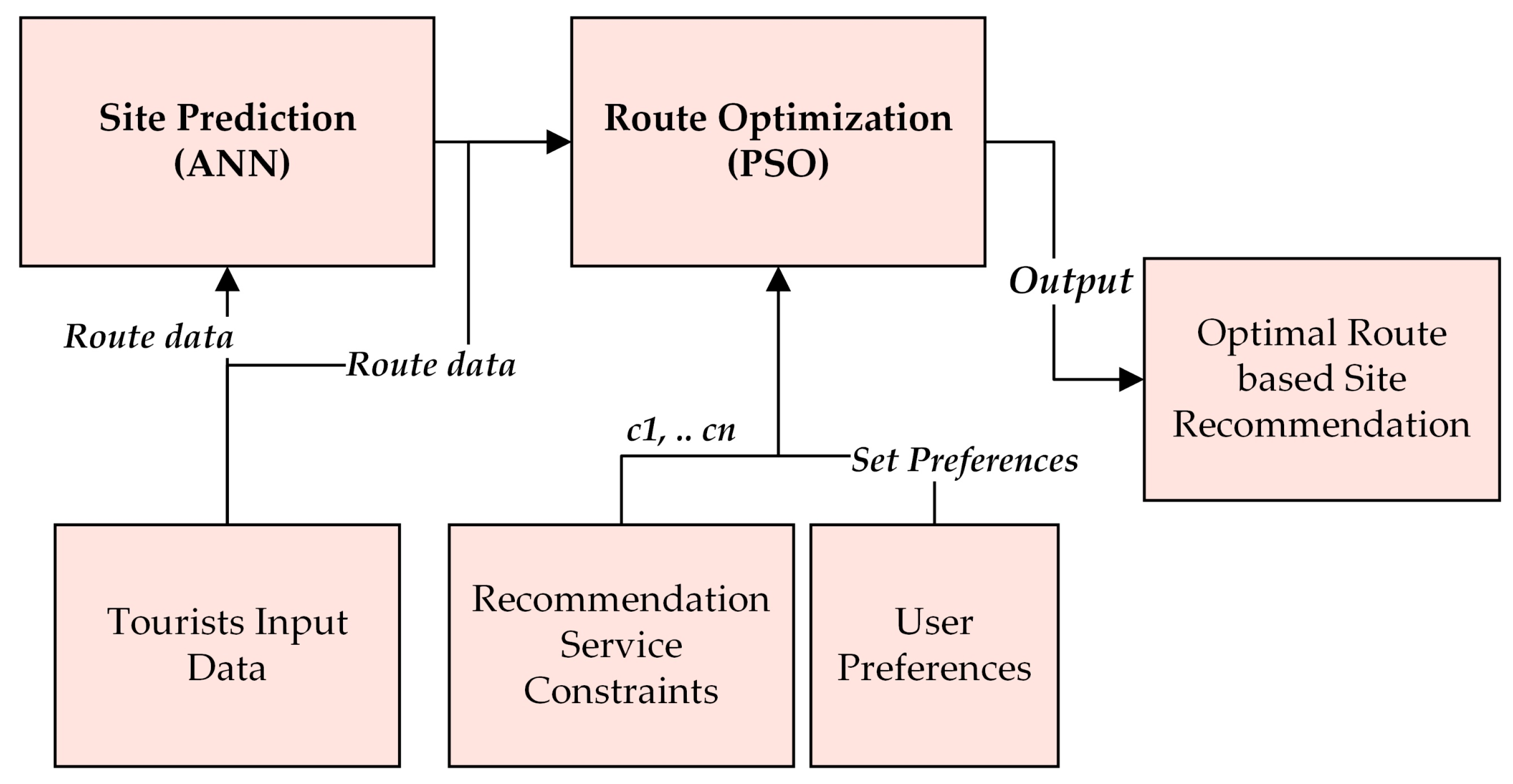
The overall system model for the proposed system is given below in
Figure 2. The tourists’ input data is taken into the site prediction module; here, predictions for recommending next site are made using artificial neural networks (ANNs). The output of the site prediction module is forwarded as input to the route optimization module along with the detailed tourist data, system constraints, and user preferences as inputs. The route optimization module takes into consideration all the given inputs and finds the optimal route to the recommended site using particle swarm optimization (PSO).
In
Section 3.1, we present the basic equations of the algorithms used for tourist site recommendation and route optimization. In
Section 3.2, we present the proposed model for an optimal route recommendation model based on site prediction and route optimization.
3.1. Algorithms Applied
In this sub-section, we introduce the basic working of two main algorithms that we have used in our prediction and optimization model.
3.1.1. Artificial Neural Networks
The research work carried out in [
40] resulted in shifting the focus to the study of artificial intelligence-based neural networks. After the dramatic increase in the processing power of computers, the use of ANNs grew dramatically, too [
41]. The artificial neural networks have two operational phases: the training phase and the testing phase. The input data is divided into two sets: training data for the training phase, and testing data for testing. In configurations of ANNs, we have to set the number of inputs, hidden layers, and output layers. Each input has a weight associated with it. First, the training phase is carried out, where the learning of the system according to parameter scenarios is performed, i.e., whether the system should fire and output under a given pattern or not. Then, in the testing phase, the accuracy for the learned system is evaluated. The output of a neuron in ANNs is calculated as shown in Equation (1) below [
42]:
where
is the output of the
jth neuron.
,
are the inputs to the neuron. The
.
wj1,
wj2, …,
wjn are the weights associated to each input.
f is the activation function, which incorporates flexibility in the neural networks.
We have used two activation functions as tanh [
43] and softmax [
44] in the implementation of neural networks, which are shown in Equations (2) and (3), respectively:
3.1.2. Particle Swarm Optimization (PSO)
The particle swarm optimization algorithm (PSO) is a population-based optimization algorithm, which was proposed in 1995 [
45]. Each particle in PSO moves with a certain velocity in a given search space, searching for an optimal solution.
In configurations of PSO, the size of the population is set along with initial positions and moving velocities. The size of the population defines the total number particles in the search space. Each particle in the PSO maintains two values: the particle’s best (pbest) value and the global best (gbest) value. The velocity of the particle is updated by using Equation (4), while the position of a particle is updated by using Equation (5) [
46]:
where,
is the particle’s velocity,
is the current particle position (solution),
is the particle’s personal best solution found so far in the search process,
is the global best solution found by any particle so far in the search,
is a random number generated between 0 and 1, and
and
are the learning factors; usually, both
c1 and
c2 are kept as 2.
3.2. Tourist Site and Route Recommendation Model
In this sub-section, we present the detailed methodology for the recommended model based on the site prediction module and optimization module.
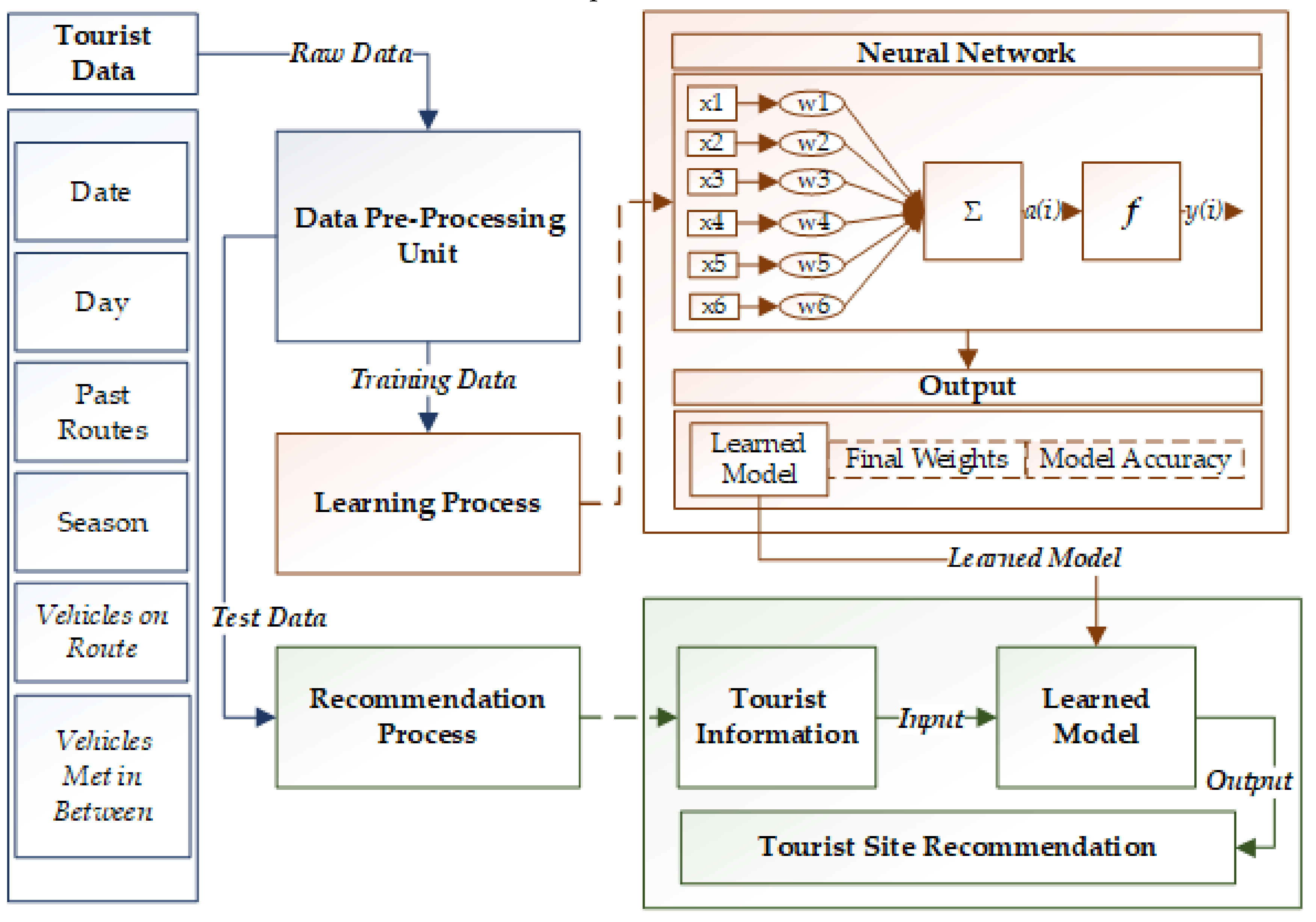
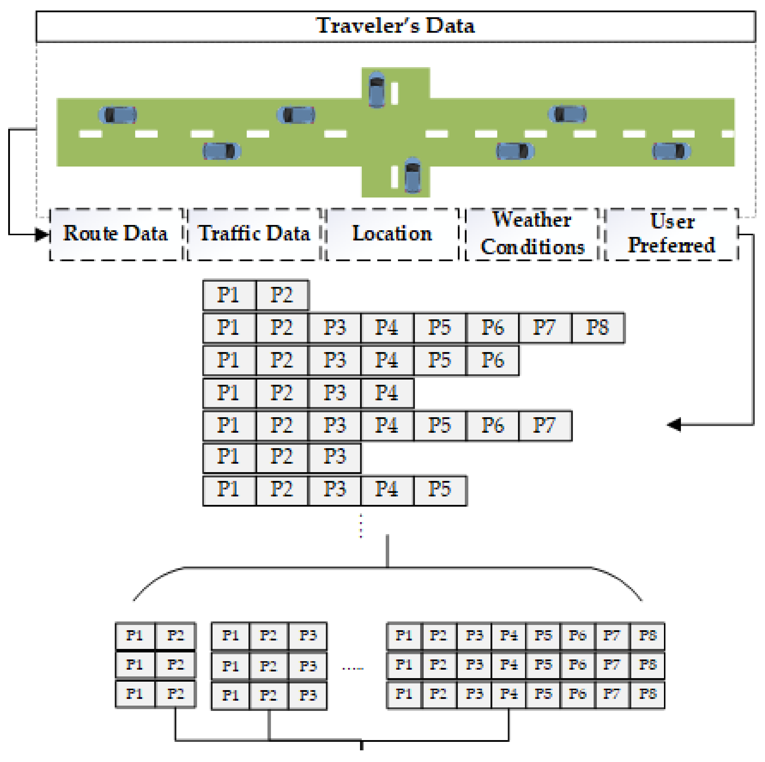
Figure 3 below shows the flow and configurations for an ANN-based site prediction module for recommending the upcoming tourist sites. First, the tourist data is given as input to the system. After pre-processing, the data is divided into training and testing modules. Training data is given as input to the learning module, where ANNs are used to prepare the learned model for the system. Once the learning process is complete, the test data is given to the recommendation module. In this phase, the site to be recommended next to the tourist is predicted.
The ANN-based site prediction module has as inputs the day of the week, day of the month (marking special days for events), season, set of past routes, vehicles on the route, and number of tourists visiting the routes in the past. The output of the module is the tourist site to be recommended.
Once the ‘best’ tourist attraction based on the learning model is selected, then, the next task of the recommendation mechanism is to find an optimal route to the selected tourist site. The output of the ANN-based tourist site recommendation module is fed to the route optimization module along with other inputs to find an optimal route to the site.
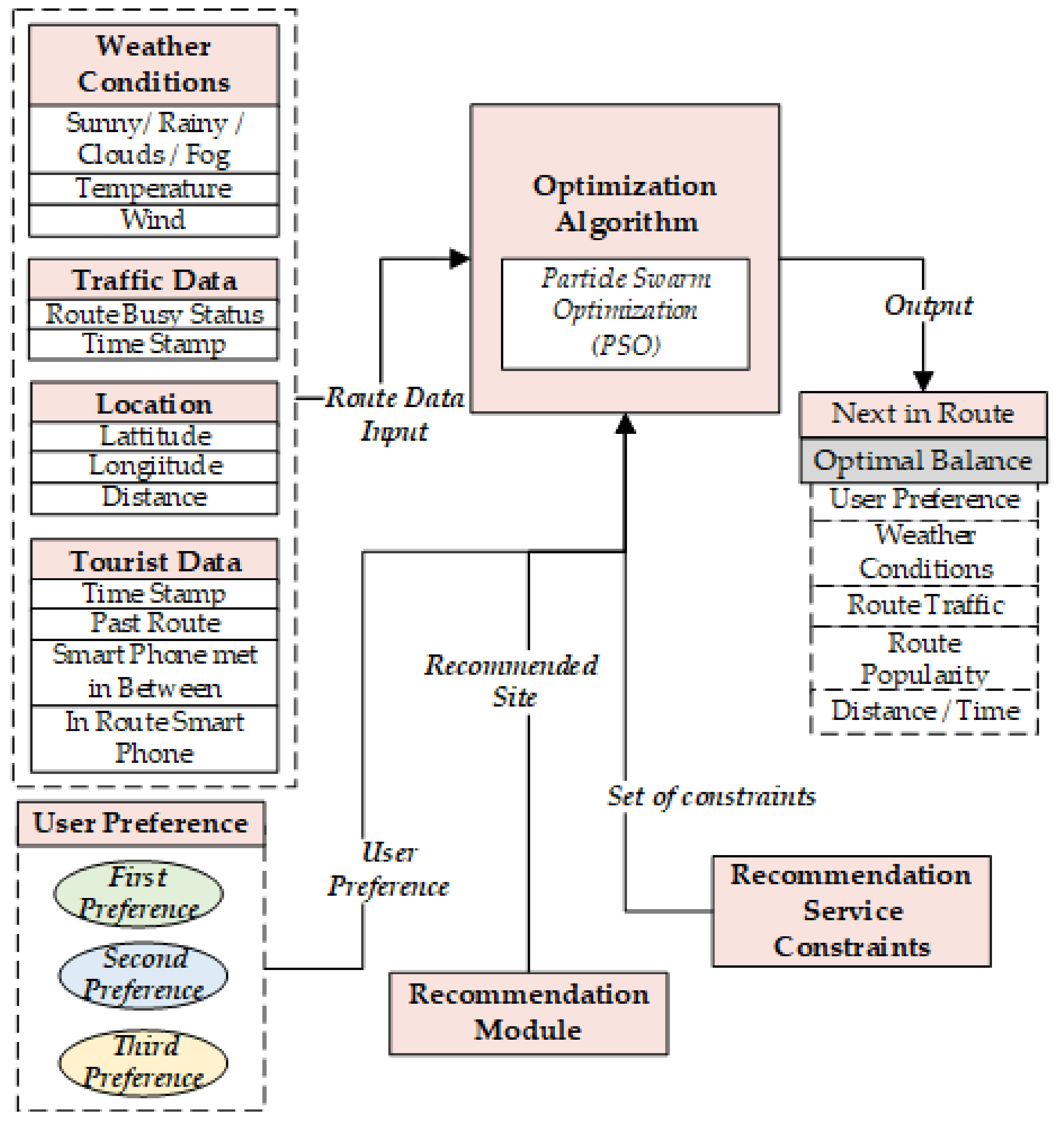
Figure 4 below elaborates the overall flow for the route optimization module. The optimization algorithm used in this module is PSO, which takes the route data, user preference, recommended site (ANN module’s output), and a set of service constraints as input. The route data consists of detailed data on all the possible points, connecting the tourist’s current location to the selected site to recommend. This detailed data compromises weather conditions, traffic data, location data, and the tourists’ data. User preference is user-input for the most desirable places and routes to visit, if there are any. The recommended site is the site selected to be recommended from the previous module. The recommendation service constraints are a set of constraints attached to some tourist sites. Constraints include visiting hours for the tourist sites for different days and different seasons, and the status of the site based on season, as some sites are open for a specific season only.
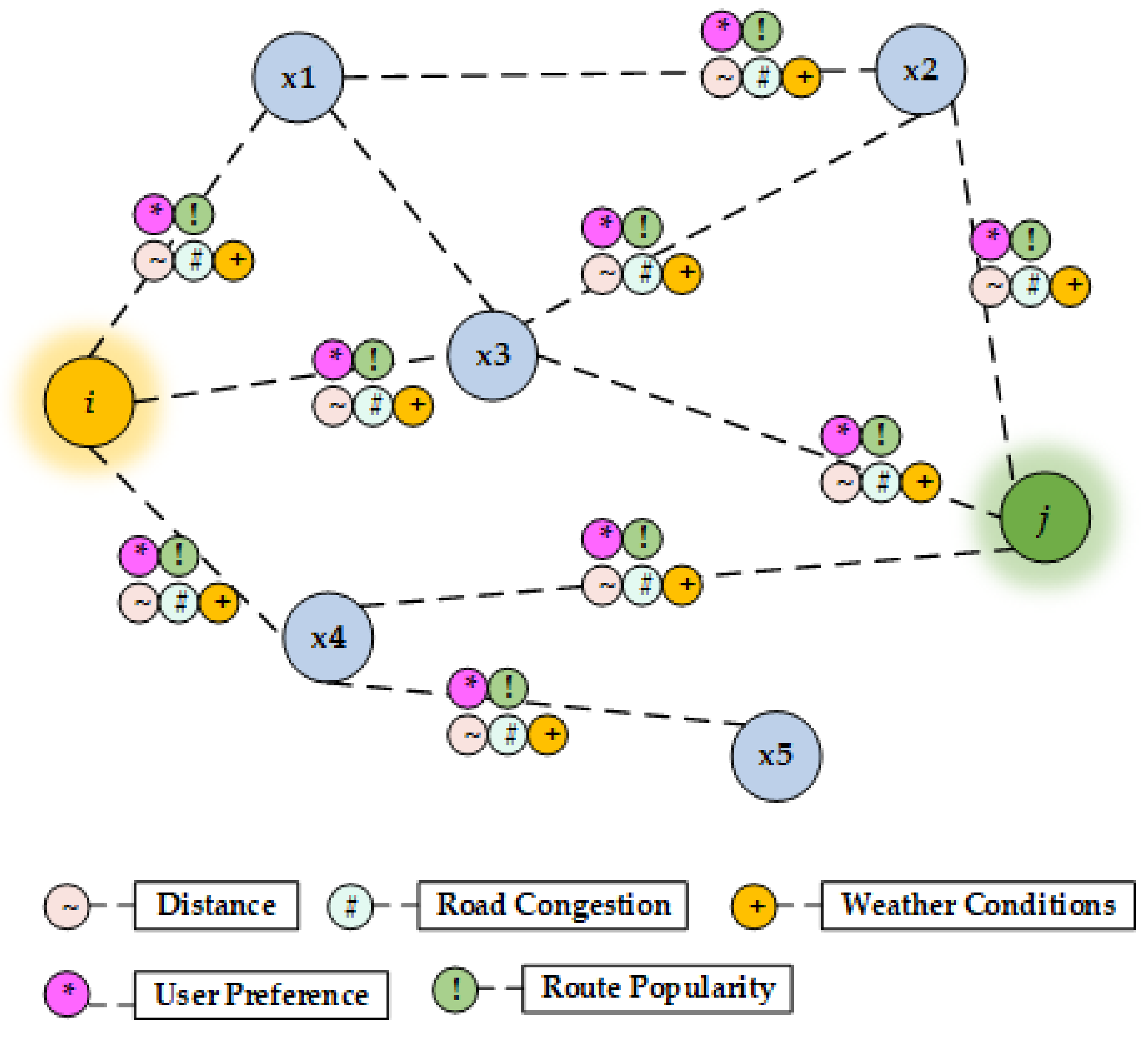
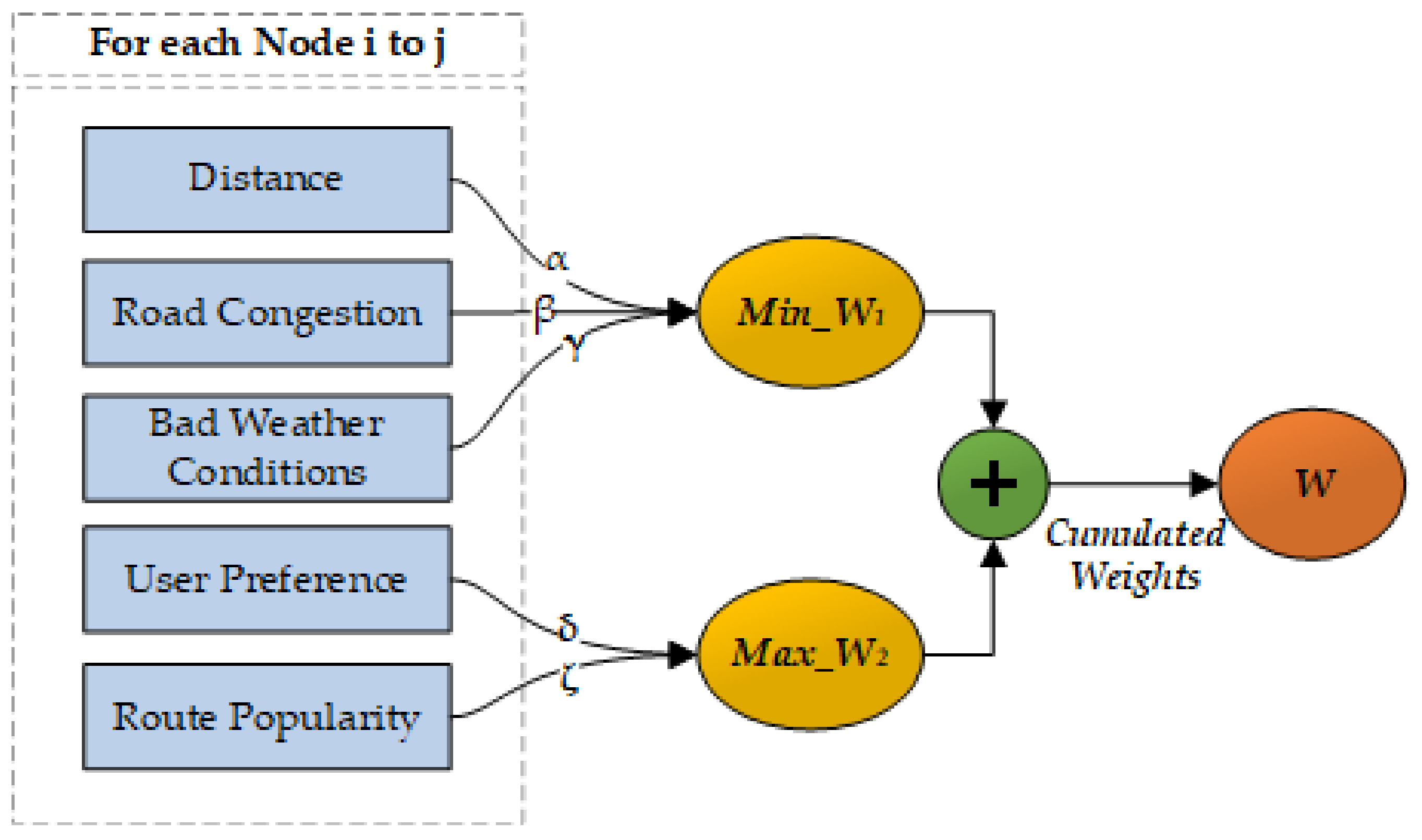
The goal of the optimization module is to achieve the best route for the tourist with optimal parameter values. An optimization algorithm needs an objective function for finding an optimal solution. Based on our input parameters and available data, we design our objective function for finding the best route for the traveler. There are five parameters extracted from the available data that are to be used in the objective function. The extracted parameters are distance, road congestion, bad weather conditions, user preference, and route popularity.
3.2.1. Objective Function for Route Optimization
First, consider two nodes
i and
j in a route, where
i is the tourist’s current location and
j is the tourist’s probable next location. The distance is the total number of kilometers that the tourist has to cover in order to travel from node
i to node
j. Road congestion is the density of traffic between the two nodes,
i and
j. Bad weather conditions are an occurrence of non-preferable travel weather conditions between nodes
i and
j. User preference is the user’s preference factor for the given link between nodes
i and
j. Route popularity is the rate at which the link between nodes
i and
j is visited by the other travelers. Note that there can be multiple links between the two nodes
i and
j, with each link having its own set of values for distance, road congestion, weather conditions, user preference, and route popularity (
Figure 5).
The aim of the objective function is to find the route to the next destination with the minimum distance, minimum road congestion, minimum bad weather conditions, maximum user preference, and maximum route popularity. Hence, we will break our objective function into two parts: one minimization function and one maximization function. The minimization objective function is given in Equation (6), and the maximization objective function is given in Equation (7).
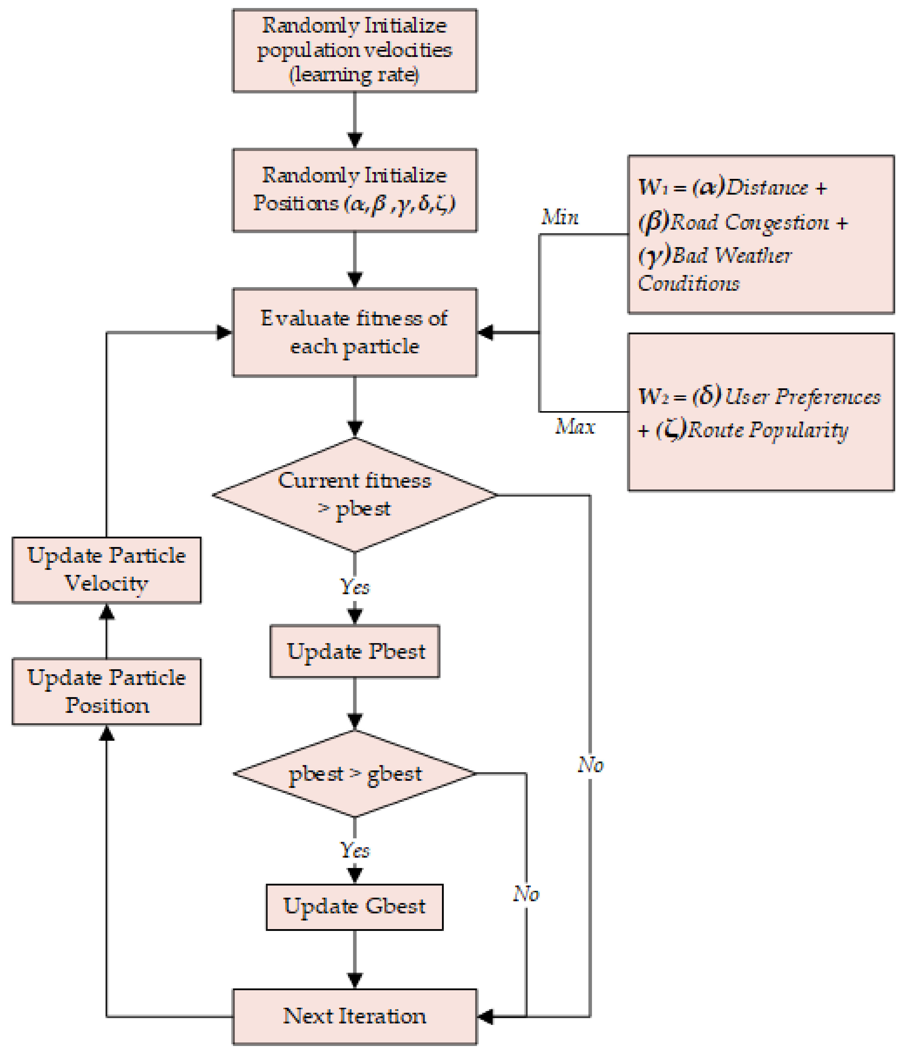
Figure 6 shows the working flow of the PSO algorithm. In PSO, first, the population particles are generated; then, the velocities and positions are initialized for each particle. Next, the fitness of each particle is evaluated based on the current velocity and position. In the fitness evaluation, we use our minimization objective function and maximization objective function. Next, the current fitness of each particle is compared to its best fitness (pbest). If the particle’s current fitness is better than its best fitness, then the pbest is updated to the current fitness; otherwise, it moves to the next iteration. After updating the pbest, the particle’s pbest is compared with the global best fitness (gbest). If the particle’s pbest is better than the gbest, then the gbest is updated to the particle’s pbest; otherwise, it moves to the next iteration. The particle’s velocity and position are updated in each iteration to calculate the new fitness values.
In Equations (6) and (7),
and
are the weights associated with the traffic data parameters of distance, road congestion, bad weather conditions, user preference, and route popularity, respectively. The goal of the objective function in PSO is to minimize the weights of distance, road congestion, and bad weather conditions in Equation (6) and maximize the weights of user preference and route popularity in Equation (7). Our final objective function can be described as given below in Equation (8) (
Figure 7):
3.2.2. Efficacy of Route Parameters’ Selection
We have a total number of five route parameters: distance, road congestion, weather conditions, user preference, and route popularity. All of these parameters play a vital role in the selection of the route from a starting point to a destination. As shown in
Figure 5 above, there can be multiple available routes from a source to a destination. Our goal as described in the objective function above is to find a route that maximizes the good route parameters, such as user preference and route popularity, and minimizes the bad route parameters, such as distance, road congestion, and bad weather conditions.
Table 1 below elaborates each parameter’s optimization goal along with its effectiveness in route selection. We have described the usefulness of parameter selection in terms of saving travel time, avoiding any additional travel fatigue, safely traveling, and improving the travel experience. In route optimization, selecting a route with optimized distance, road congestion, and weather conditions can result in saving travel time for the tourist and giving more time for sightseeing. Also, the selection of routes with less road congestion and minimum bad weather conditions will save tourists from any additional travel fatigue. Avoiding the extreme weather conditions will also make traveling more safe. For example, in winter, there are routes that might have high snowfall, and thus are not recommended for safe travel. Adding the features of user preference and route popularity will allow tourists to visit top tourist sites along with the ability to get a customized travel experience. In
Table 2, Yes/No refers to whether the selected parameter might provide the considered benefit in some cases or might not provide in other cases, depending on the scenarios.
There can be different scenarios of a route depending on the values of road congestion, weather conditions, route popularity, and user preferences.
Table 3 below shows the classification of the data scenarios for better understanding the route optimization process. Each scenario class follows the parameters of road congestion, weather conditions, user preference, and route popularity, and is drawn based on set upper and lower threshold values that are derived from the collected data.
5. Results Analysis
In this section, we present the results analysis of our proposed route recommendation mechanism based on PSO and ANNs. In
Section 5.1, we present the initial recommendation accuracy of the recommendation module using ANNs. In
Section 5.2, we present the route optimization results for the tourist site recommendation. In
Section 5.3, we present the comparisons of the genetic algorithm (GA) for the optimization with PSO.
For prediction-based recommendations using ANNs, we have divided our dataset into two subsets: a training set and a testing set. We have taken 75% of the data as the training set and 25% of the data as the testing set. We have six inputs, six hidden layers, and one output in the applied ANN implementation.
In PSO implementation, we have used a total number of 17 particles in the search space. The search space position array for the PSO particles holds a combination array for and .
5.1. ANNs Prediction Accuracy Based on Route Size
In this sub-section, we present the performance results of site prediction on the tourist’s data. As mentioned in
Section 4.1, in pre-processing, we separate our data based on route size.
As we have earlier discussed in
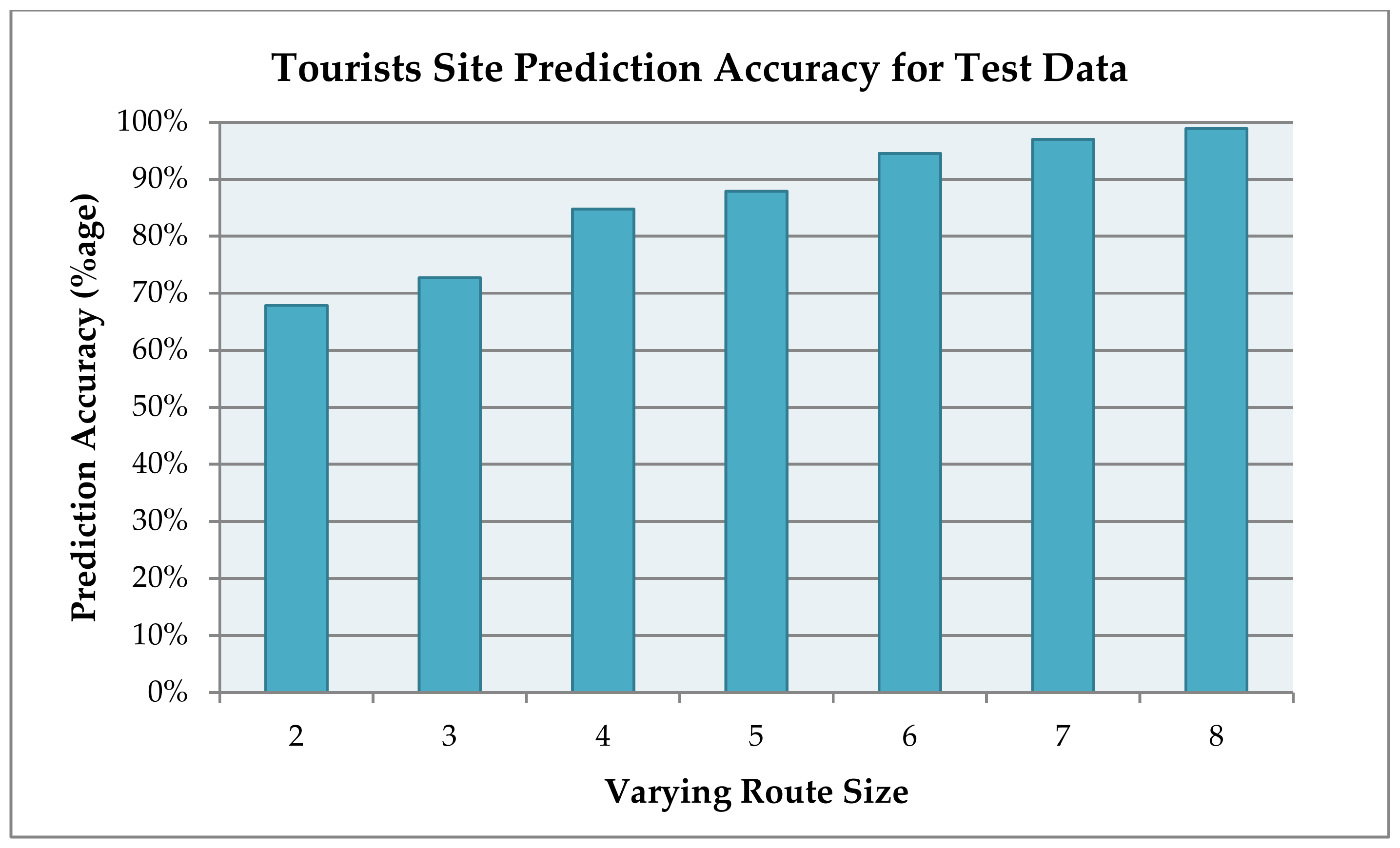
Section 4.1, that dataset consists of multiple tourist trips spanning over a time period of one year. Each tourist trip can cover multiple locations each day; the number of tourist locations covered in a day during a tourist trip is referred to as the route size. We have route sizes ranging from two to eight. In our learning-based prediction model, if we give x number of tourist sites covered so far to the system as input along with other required input parameters, the system should be able to predict the most likely tourist site to be visited next.
In
Figure 9, the results of the prediction accuracy for varying route sizes are shown. The prediction accuracy for a route size of two is around 68%, reaching up to more than 99% for a route size of eight. For smaller route sizes, the learning of the system becomes very limited. In contrast, when the input route size is high, the training phase is improved with more data, and the error rate is subsequently reduced.
The system is robust against large numbers of route sizes. Although our available data is up to the size of eight routes size only, for system performance insurance purposes, we have generated the large route sizes test data with the use of available data. The system ensures the accommodation of larger route sizes, and works efficiently for higher route sizes, too.
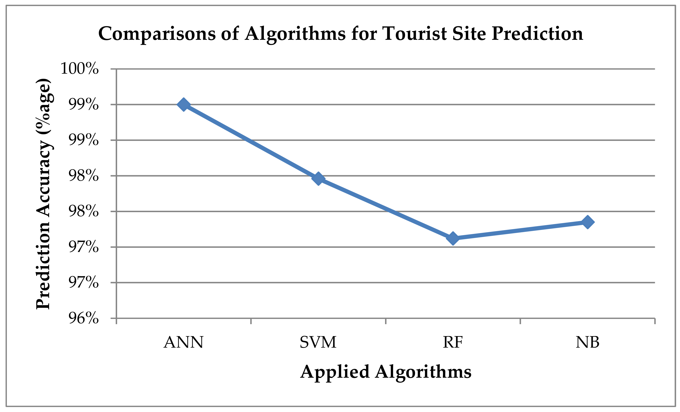
The comparisons of prediction accuracy for prediction algorithms as ANN, SVM, random forest (RF), and naive Bayes (NB) are shown in
Figure 10. The results show the average prediction accuracy for multiple iterations of test data with route sizes of six, seven, and eight. It clearly shows in the results that ANN proves to be the best fit in the given problem scenarios, as it gives the maximum prediction accuracy.
The learning mechanism for prediction is also done based on seasons and special annual events, too. The tourist site results vary depending on the season and whether the given day is any special day of the year. An example of an event-based prediction and season-based prediction for site recommendation is given in
Table 6. Since our dataset is of Jeju Island, in October, the Chisimni festival is held in the Seogwipo City of Jeju Island, and in March, the cherry blossom festival is held in Jeju Island. Hence, the recommendations to the tourists will be based on special events and season-based learnings.
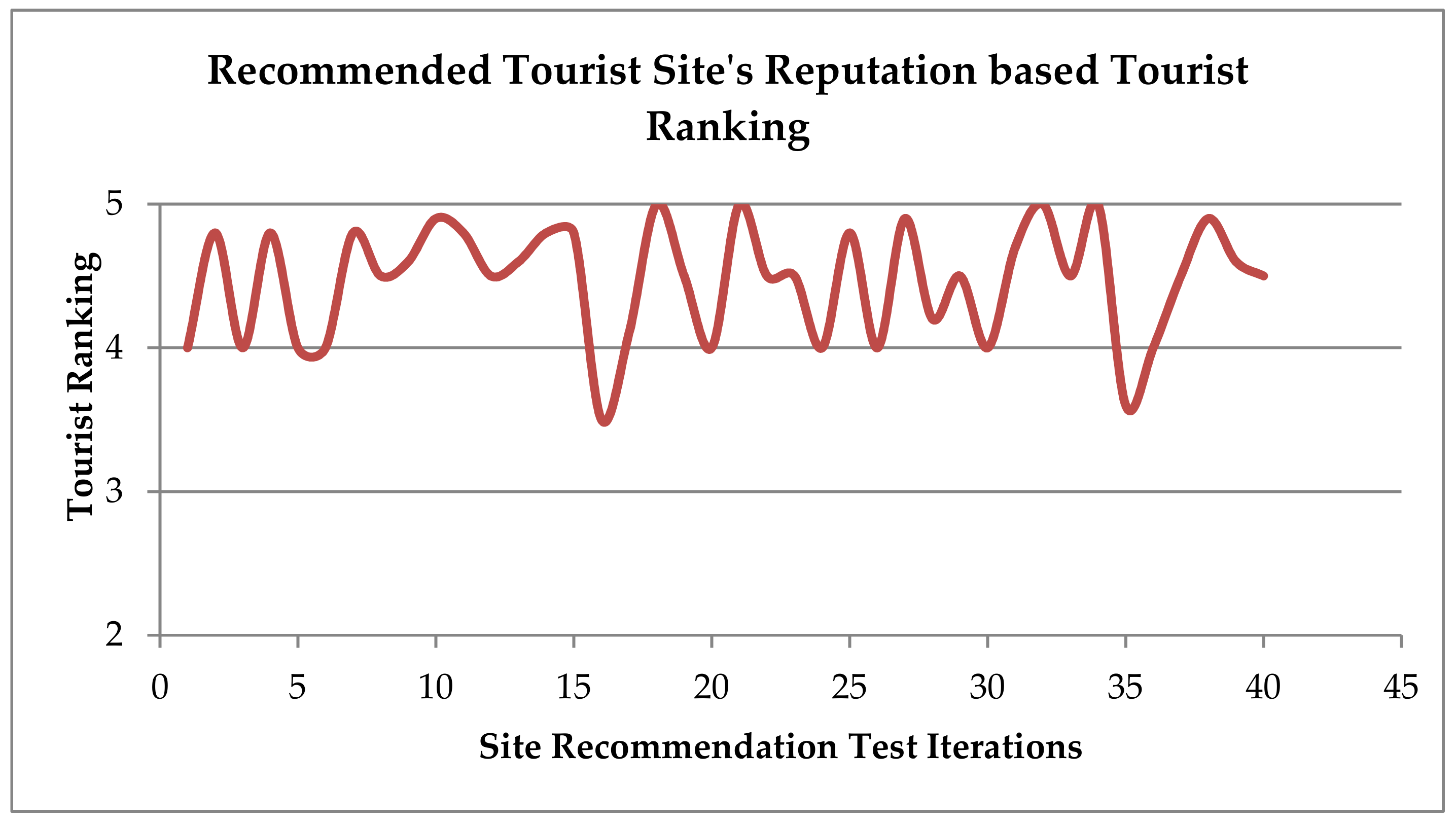
The selected sites for recommendation, as a sample shown in
Table 5, are cross-referenced with tourist opinions extracted using Naver and TripAdvisor. Naver is a South Korean online platform that is widely used in South Korea and has more records available.
Figure 11 shows the mapping of recommended sites onto the tourists’ ranking obtained from Naver and Trip Advisor. There are five rankings: 0–1 (Terrible), 1–2 (Poor), 2–3 (Average), 3–4 (Good), and 4–5 (Excellent). We can observe that most of the recommended sites fall into the good and excellent categories of tourist rankings.
5.2. Tourist Site Recommendation with Route Optimization
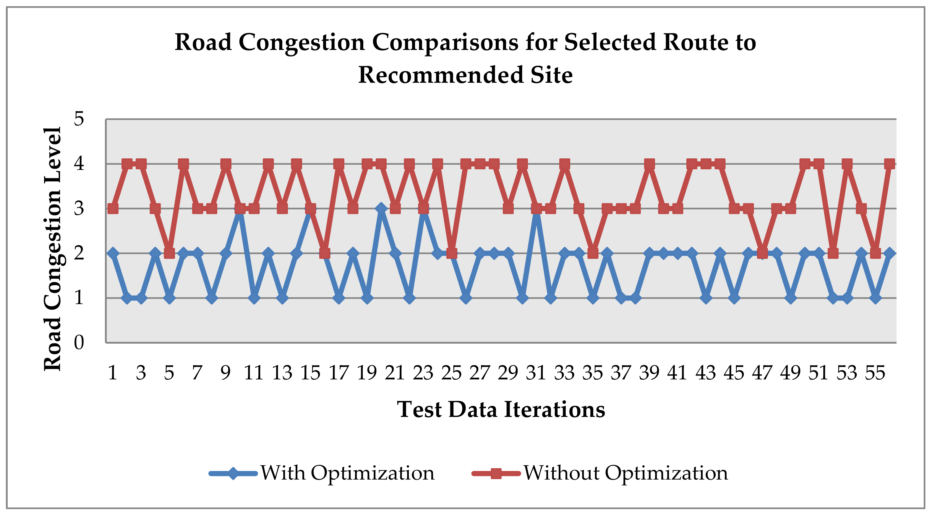
In this sub-section, we evaluate the results of our proposed optimization technique for the route optimization of tourist site recommendations. The optimized system is compared with a non-optimized approach, where the tourist site and route is recommended based on the learnings from the prediction module only. We map the obtained results into the classes presented in
Table 1 except for distance, which is directly represented in kilometers, for better understanding the difference between the optimized routes and non-optimized routes.
Figure 12 below shows the results for the road congestion level of the selected route to the recommended site. In road congestion, we have five levels—0, 1, 2, 3, and 4—representing very low traffic, low traffic, medium traffic, high traffic, and very high traffic, respectively. Each class of road congestion basically shows the traffic density level at the selected route. The proposed optimization algorithm aims to minimize the level of road congestion to save the tourist’s time and travel fatigue. In the figure, we can observe that the road congestion drops one to two levels with route optimization in comparison to the non-optimized route.
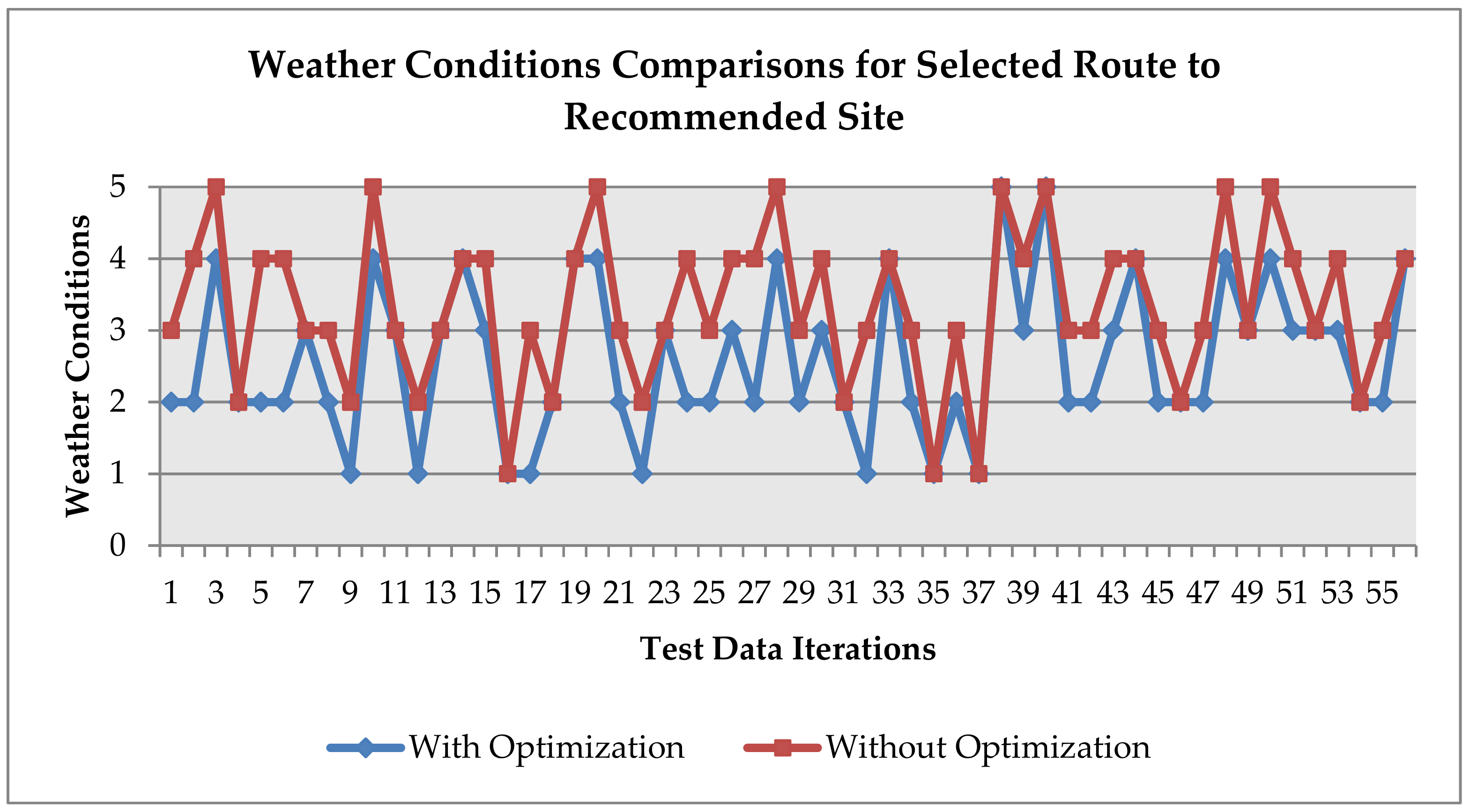
Figure 13 below shows the weather conditions comparisons, for the selected route to the recommended site, of optimized and non-optimized solutions. In weather conditions, we have five levels of 0, 1, 2, 3, and 4 representing very good weather conditions, good weather conditions, average weather conditions, bad weather conditions, and very bad weather conditions (
Table 1). The optimized technique showed some improvement in the weather conditions as compared to the non-optimized approach, but the difference is not very high. Since the collected data is based on Jeju Island, which is a comparatively small island based on two cities only, the weather conditions can only be improved when the route has to be taken from one edge of the island to another. Regarding short routes, the weather conditions remain almost the same on alternative routes.
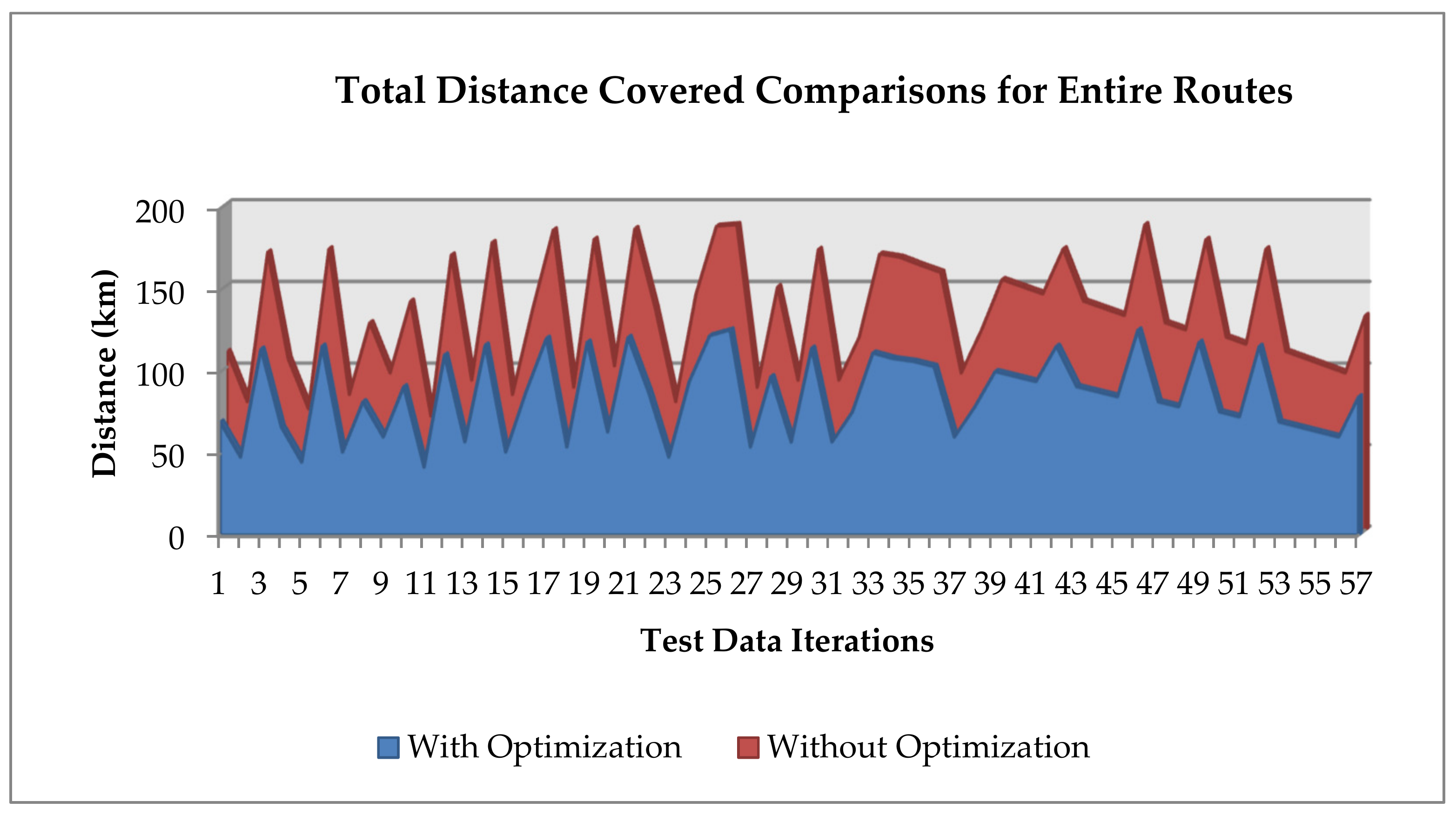
In
Figure 14, we present comparisons between the optimized and non-optimized approaches for the total distance covered. The total distance refers to the sums of distances covered by a tourist over a whole day’s route, considering all the stops, depending on the route size. Our proposed optimization technique considers distance as one of the important factors, as it is directly proportional to the time taken. Hence, the proposed technique best optimizes the set of tourist sites to be recommended in a manner that takes the least overall time.
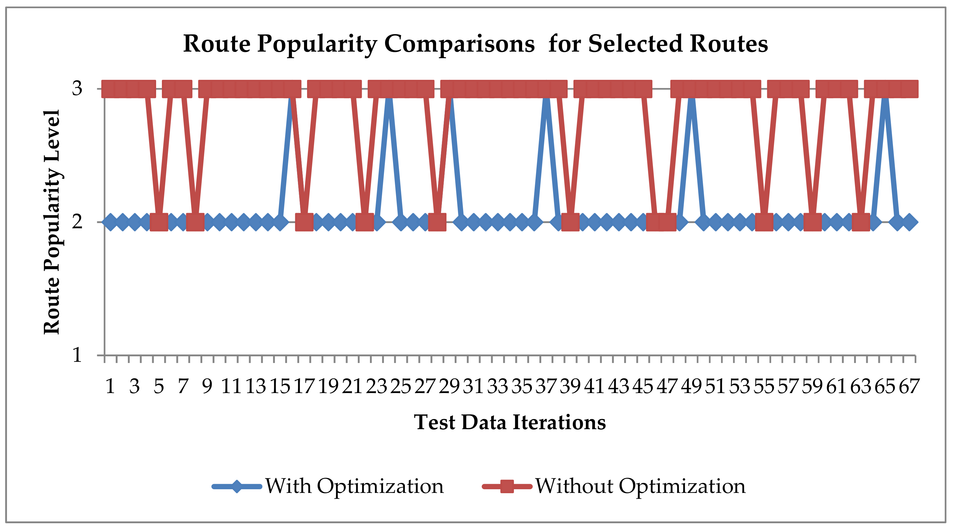
In
Figure 15, we compare the route popularity levels among the optimized and non-optimized approaches. In the figure, we can observe that the non-optimized approach targets the highly popular routes most of the time, while the optimized approach lies at the medium popular route mostly. Since the optimal approach considers other factors such as minimizing the distance, road congestion, and bad weather conditions, it finds an optimal balance between the route popularity instead of targeting the highest popular route and failing at the minimization function. Similarly, regarding user preference, a behavior identical to the route popularity is observed. However, both route popularity and user preference can be given a forced high weightage in any such preferred scenarios, if required.
In order to keep an optimal balance between the maximization and minimization parts of the objective function, the maximization function for maximizing the route popularity and maximizing the user preference settles near average levels in order to perform best at minimizing the distance, minimizing the road congestion, and minimizing the bad weather conditions. The optimal balance between the weights of five optimization factors varied depending on the different input scenarios.
Table 7 below shows most recurring set of weights ranges for the optimization factors.
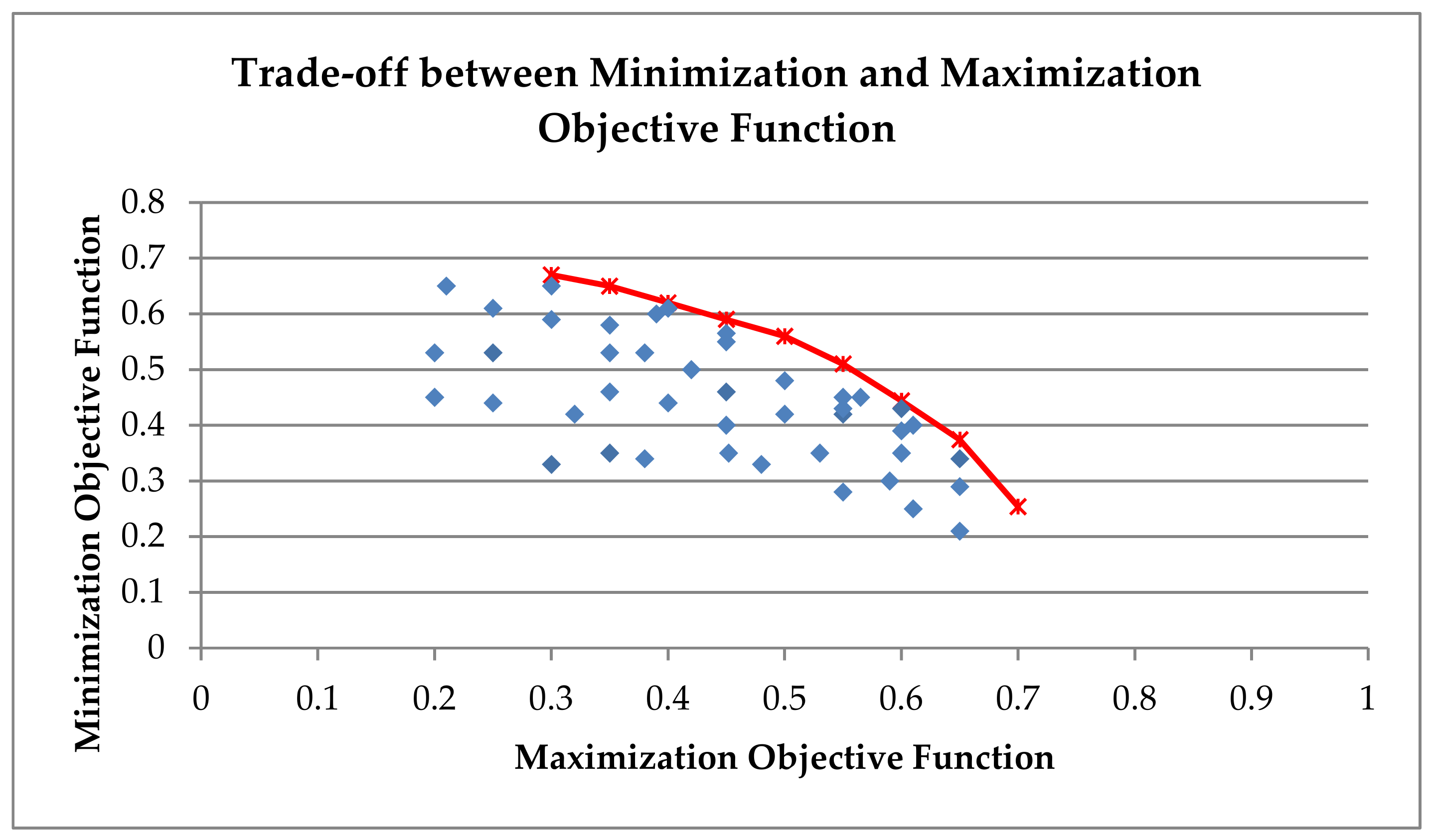
Figure 16 shows the Pareto front for the optimization minimization and maximization functions. The Pareto front is an area where one parameter’s criteria cannot improve without worsening another parameter’s criteria. In many scenarios, the optimization algorithm has to make optimal tuning between minimization and maximization, as improving one can have an effect on the other. The red line in
Figure 16 shows the Pareto frontier, which presents the set of the optimal solution points’ trade-off between minimization and maximization.
5.3. Scenarios Case Assumptions
In this section, we make assumed scenarios for the optimization parameter values and test their output for the proposed system.
5.3.1. Scenario 1
If a parameter value is at the same level (best or worst) on all the possible routes to the recommended site, R
1, R
2… R
n are the possible routes between two points P
x and P
y:
where,
X = {
. If Equation (9) is true, then the parameter weightage for the
X parameter behind X will be set as zero, i.e., {
.
In order to test the given scenario, we take a starting point P
x and a destination point P
y from our dataset
. We have taken a sample set of points (P
x, P
y) that have five possible routes from starting point P
x to destination P
y. We set the same values on all five routes for the parameters of road congestion and user preference. Now, in this scenario, the parameters of road congestion and user preference are set to 0 throughout, as they have the same values over all five routes. The route optimization decision is made based on the parameters of distance, weather conditions, and route popularity. In
Figure 17, we can clearly observe from the results that route four is the most optimal route of the available five routes. For route four, we can find a clear balance among all three parameters of distance, route popularity, and weather conditions. Route one can be preferred over route four if the user chooses to settle at a considerably less popular route as a trade-off for slightly better distance and weather condition values. For route three, the weather conditions are bad, and also the route popularity is low. For route five, the distance is the smallest, but the route popularity and the weather conditions are at their lowest too among all the available routes.
5.3.2. Scenario 2
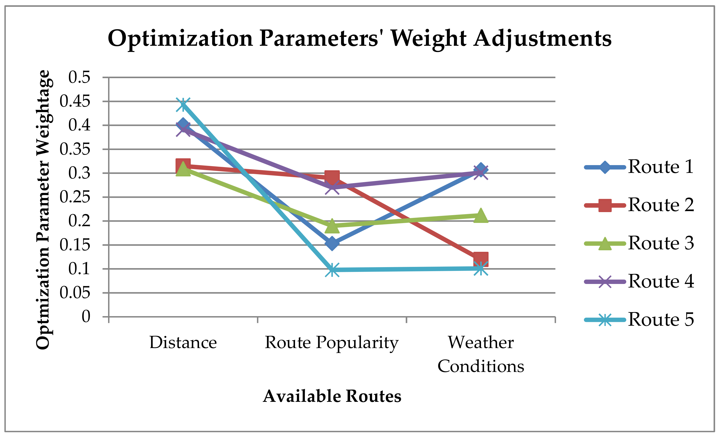
The second scenario is defined as whether the user has assigned a high weightage to any parameter: distance, weather conditions, road congestion, route popularity, or user-preferred route. We have assumed a high weightage for user preference to be between the given ranges as below.
where,
X = {
. The user can fix any parameters’ weightage as high between the given ranges of 0.4 to 1.0.
We have tested the available data by fixing each one of the parameter’s weightage to 0.5, one by one. In
Table 8, we present the average weight adjustment results for scenarios where one of the parameters is fixed at a higher weightage. Once a parameter is fixed at a high weightage, the optimization process would make its best effort to find an optimal balance among the other available parameters. In
Table 8, we can observe how the weights are fluctuating with each test scenario, but also result in finding a fair distribution among the remaining parameters.
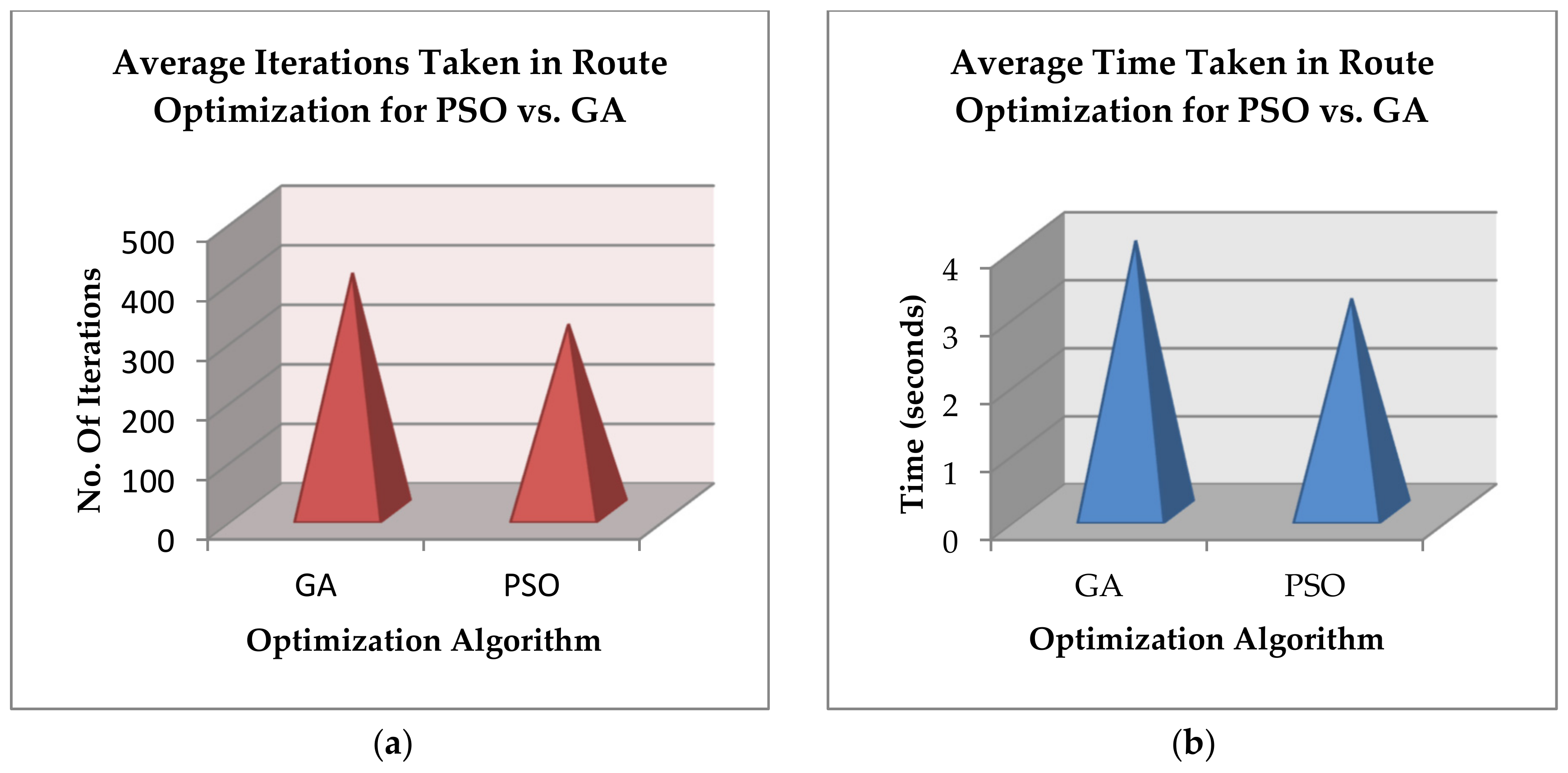
5.4. Comparisons of GA vs. PSO
In this sub-section, we compare the optimization results of PSO with GA. In our implementation of GA, for holding the comparisons, we used the same system environment as used for PSO.
Both the algorithms gave same optimized route as output using the proposed objective function. The difference seen is in the performance levels of both the algorithms in terms of the total number of iterations performed and the total time taken for the optimization process. The total number of iterations is the number of turns that an algorithm takes to find the best positions for particles in the case of PSO and the best crossover and mutation rate in the case of the GA. As we can clearly observe in
Figure 18a below, the average number of iterations taken by the GA is much higher in comparison to that of PSO. Similarly, since GA takes a larger number of iterations to find the optimal route, hence, it also takes more time for the optimization process, as shown in
Figure 18b.
6. Comparative Analysis and Discussions
Tourist sites mostly are widely known; also, information and rankings can be found on online forums. Data found on online forums might not be all authentic; also, it’s a hectic job for the tourist to search for tourist sites, make a list of points to be covered in a day, and manage the time accordingly. Mostly, the tourists have to be dependent on the travel guides for a multi-point day trip. In our proposed system, we target building an on-the-spot recommendation system that continuously updates the recommendations as the tourist’s location changes based on the tourist’s current data and past tourism data that is fed to the system. The goal of the proposed work is to make tourism flexible and easy, with point-to-point site recommendations and route optimization.
In this work, we have presented a mechanism for predicting a tourist’s probable next location and provided an optimal route recommendation to the site. Previously, many works have focused on site recommendation and route recommendation, but the optimal route to the next destination, considering all involved factors, has not been given much attention.
Table 9 below gives a comparison between previously proposed recommendation systems and our proposed recommendation system. Most of the related works for route recommendation focus more on the parameters such as user preference and distance, while very few studies have focused on approaches based on route popularity and weather conditions and visiting time constraints. To the best of our knowledge, our proposed system is the first of its kind in considering all six input parameters of user preference, distance, route congestion, route/site popularity, weather conditions, and visiting time constraints.
Regarding the comparisons above, it can be clearly seen that one study [
55] considered just one parameter of preference. The combination of two parameters of preference and route/site popularity is covered by two studies: [
53] and [
56]. The combination of two parameters of preference and distance is covered by four studies: [
48], [
50], [
52], and [
58]; whereas the study in [
49] adds a third parameter of route/site popularity, the study in [
51] adds a third parameter of weather conditions, and the study in [
54] considers a third parameter of road congestion. The study in [
57] considers the parameters of preference and visiting time constraints. In total, out of the six optimization factors, only three studies consider a combination of the three optimization factors, which is the maximum number considered factors in the above comparisons, excluding our proposed system. The optimization factors make a clear impact on the optimization outcome, as the results are derived in accordance to the considered factors in the optimization process. For example, if weather conditions are not considered, the system might suggest a place that is under the effect of heavy snowfall or heavy rain, which might make the experience miserable for the tourist. Similarly, not considering road congestion might waste many hours of the tourist on traffic jammed roads. Visiting time constraints allow the recommendations be made in accordance to the opening hours and working days of the tourist spots and facilities. Distance, road congestions, and weather conditions factors make an effort to save a tourist’s time and avoid travel fatigue. Preference and route popularity are applied to improve the tourist’s experience based on personal priorities and popular feedback. Hence, each optimization factor has its own significance, and the outcome of the recommended route can be hugely affected by the factors that an optimization algorithm takes into consideration during the processing phase. Therefore, we can conclude from above comparisons that our proposed system makes its best effort to cover all the possible scenarios and save the traveler from any bad experience.
7. Conclusions
A sustainable tourist experience is one that can cope with the continuously changing travel conditions. The rise of the tourism industry has shifted the research focus on tourism-based recommendation systems. Many efforts have been done in the provision of better prediction and recommendation systems for tourists in the last decade. Tourist attraction prediction and optimal route recommendation is a tricky problem, as many factors get involved in the finding of an optimal route. These factors also keep on changing depending on different tourists and location scenarios.
In this work, we have made an attempt to address two of the main factors of travel as sightseeing and route selection for traveling to the tourist site. We propose a recommendation system based on a next-tourist attraction prediction module and route optimization module. We also pay profound attention to listing most of the possible factors involved in route optimization. A popular sight alone out of context cannot be recommended, as it is not necessary that a sight that is popular in March is also popular in August, since many of the tourist sites in the world have seasonal and timeline dependencies. Hence, the recommendable tourist sites keep changing throughout the year. In the recommendation process, based on past tourists’ data using the learned model, a recommendation is made for the most likely site to be visited for the tourist. The recommendations are made in accordance to the special events in a year, weekends, and popular tourist spots with respect to the seasons. In the prediction module, we use ANNs. In the optimization module, we use PSO to find the optimal route for a given set of input scenarios. In our route optimization, we have five main factors under consideration: distance, road congestion, bad weather conditions, route popularity, and user preference. Our optimization aims to minimize the weights for distance, road congestion, and bad weather conditions as a tourist would want to save time on routes and spend more time at the destination and enjoy the views at the tourist site instead. In results analysis, we have compared the performance of the optimized and non-optimized approaches. We have also compared the performance results of our chosen PSO algorithm with GA optimization technique. The results analysis and performance comparisons demonstrate that our proposed system is ideal, as it takes into account most of the crucial factors between the two links of a route, putting forward the best effort for an optimal route recommendation.
Our main contribution in this work can be summarized as a context-based recommendation system and a best effort route optimization. The limitations of the system can be cases where we do not have enough data to feed to the system. In the future, we aim to continue the problem and explore better solutions regarding data limitations.


