The Scale-Dependent Behaviour of Cities: A Cross-Cities Multiscale Driver Analysis of Urban Energy Use

Abstract

Hosting more than half of the world population, cities are currently responsible for two thirds of the global energy use and three quarters of the global CO2 emissions related to energy use. As humanity becomes more urbanized, urban systems are becoming a major nexus of global sustainability. Various studies have tried to pinpoint urban energy use drivers in order to find actionable levers to mitigate consumption and its associated environmental effects. Some of the approaches, mainly coming from complexity science and industrial ecology disciplines, use city-scale data to find power-laws relating to different types of energy use metrics with urban features at a city-scale. By doing so, cities’ internal complexity and heterogeneity are not explicitly addressed. Moreover, to our knowledge, no studies have yet explicitly addressed the potential scale dependency of such drivers. Drivers might not be transferable to other scales and yield undesired effects. In the present study, power-law relations are examined for 10 cities worldwide at city scale and infra-city scale, and the results are compared across scales. Relations are made across three urban features for three energy use intensity metrics. The results show that energy use drivers are in fact scale-dependent and are city-dependent for intra-urban territories.

1. Introduction

Urban production and consumption activities are responsible for the greatest share of global resources use and pollution. Cities account for 65% of global energy use and are responsible for 71–76% of global CO2 emissions [1]. More than half of the global population already lives in cities, and by 2050, cities are projected to host 80% of the global population [2,3]. If current consumption and production patterns remain the same, the environmental impact of cities is likely to increase significantly. For these reasons, cities are pointed to as both a future major problem and solution to global sustainability challenges [4,5]. Therefore, it is urgent to reduce the environmental impact of anthropogenic activities in order to remain within a safe operating and balance space for humanity [6] by setting the most appropriate pathways for urban resource consumption mitigation.

In this matter, Grubler et al. (Global Energy Assessment) [7] argue several points regarding the selection of the best pathway for the mitigation of urban energy impact. Firstly, when considering urban systems in an exergy analysis, they are far (<20%) from reaching their thermodynamic efficiency frontier, which implies a theoretical improvement in energy demand. Secondly, due to the large difference between the density of the energy demand in cities and the density of possible on-site energy supply (10–100 W/m² versus 0.1–1 W/m² [7]), the local renewable energy harvesting might only provide for a few percent of urban energy demand in the best cases (e.g., <1% for megacities and a few percentage points for smaller cities). Thirdly, systemic changes in the management of urban energy use usually have better leverage in the long run to reduce energy use than technological end-user level improvements. This points towards a more holistic approach of the energy use in cities and its mitigation.

Numerous researchers have looked for potential patterns in urban resource and energy use (intensity) in the past years, in order to identify generalizable drivers and to propose mitigation strategies, with great diversity in approaches. The following studies are not directly comparable to the approach developed in the present paper (see “Section 2.2 Method”) but should however be mentioned to give the reader an overview of other approaches with similar purpose. These studies varied in scope and methodological and accounting approaches, and therefore resulted in different policy recommendations. Publications identified drivers of final [8,9,10], primary, direct or territorial-based [11,12,13,14,15], indirect or consumption-based energy uses [16,17,18] using top-down [19,20], or other modelling [21,22] and accounting approaches [23]. Publications identifying final energy use [8,9,10] via multivariate regressions and econometric forecasting show that, among other factors, urban form, economic activity, and income can impact final energy use in residential and transport sectors. Other studies [11,12] show growing trends in primary energy use via long term temporal comparative quantitative analysis. The studies focusing on direct or territorial-based consumption [11,12,13,14,15] carry out regression and correlation analysis including a multitude of factors in their methods (such as GPD, land area, population, population density, heating degree days, floor space) to explain differences in direct energy use. It appears from the literature [8,9,10,11,12,13,14,15] that different sets of drivers are found depending on whether the energy use is measured in final, primary or direct accounting, even though they are all representative of urban energy use. This underlines the importance of accurately defining the energy use indicators that are examined before generalising about the drivers. Among those studies, only two [13,14,15] use infra-urban data in their analysis and only for one city. Another set of studies [16,17,18] give an estimation of the indirect (or consumption-based) energy uses across the global hinterland. These figures are the result of combining household expenditure data with input-output tables which are usually available at country-scale, and therefore often downscaled at a city-level. The main limitation of this approach is that driver identification is heavily biased in regard to household expenditure and therefore the energy use drivers are similar to income and expenditure drivers. Top-down approaches [19,20] compute energy-use values by taking national energy use accounting and downscaling them to city-scale based on urban population size compared to national population. This limits greatly the soundness of driver identification as it assumes a linear relation between energy use and population size, introducing once again an important bias. Other modelling approaches [21] predict energy use by end-use (e.g., heating) at high resolution (i.e., block level) based on surveys and disaggregation of zip-code level energy use data. The main limitation of such an approach lies on the assumptions necessary to create the model (e.g., buildings’ function are the major factor of energy use). Some other research has combined consumption based accounting and multivariate regression analysis to determine the impact of urban sprawl (i.e., population density) on energy use [22]. Finally, another study compares approaches between direct and indirect accounting [23] to conclude that, although indirect accounting provides the global-level assessment of energy use along the production chain, direct accounting is valuable to understand its relationship to urban systems besides expenditure-related drivers. A table providing granularity, energy vectors and urban factor studied, method and main findings of each previously mentioned article can be found in Supplementary Material, Table S1. Each of these approaches used various types of sources for their data (including surveys, statistical reports, household budget surveys, input-output tables), targeting different levels of analysis (from the household level to city or even country level) and therefore yielding results with various levels of certainty on the identification of energy-use drivers. It can be argued that this emerging research trend (partially covered by the industrial ecology discipline) has been fuelled by the increasing availability of data at the urban level [24]. However, the above-mentioned literature either relies on modelled data and a series of assumptions, or compares a great number of urban systems at a city level while considering them as homogeneous entities, or, finally, compares intra-urban territories but only for a specific city. A study comparing multiple cities worldwide across scales (infra- and city-scale) and relying on metered data is still lacking.

A more recent research approach is being developed around what is sometimes called the new science of cities, which strives to analyse cities all around the world as complex systems, driven by universal laws shared by all cities, that emerge on a “macroscale” (city-scale) from local level interactions [25,26]. Based on univariate correlations on real-world data, this research community provides a theoretical framework capable of predicting the evolution of a series of urban characteristics based on cities’ sizes. More specifically, these studies focus on analysing how urban infrastructure, socio-economic or metabolic indicators change with either the population or the mean population density (e.g., [14,27,28,29,30,31,32,33,34,35,36,37,38,39,40,41,42,43,44,45]). These studies suggest that, even though cities seem to be very complex, different from one another and being located in very different regions of the world, they might share common macroscale (city-scale) simple behaviours. Regarding the intensity of urban energy use and scaling laws, Facchini et al. [14] show that the 27 megacities worldwide (with over 10 million inhabitants) follow a power-law between urbanized population density and per capita (total) energy consumption (R² = 0.74). This result suggests that population density might be the (single) major driver of the intensity of energy consumption in urban systems, regardless of their location on the globe. Additionally, Lemoy and Caruso [34] show that European mono-centric cities display scaling of their radian profile of population density, suggesting that cities’ density profiles are homothetic. These two findings put together might suggest that the internal scaling of urban energy use can be found, allowing to overcome the a-spatial approach of current “scaling laws” of cities.

Previous “scaling law” studies are generally based on data on a macroscale (city or metropolitan) level. By doing so, cities are often considered as homogeneous and a-spatial [34] entities reducing the complexity of their functioning [46]. Yet, cities are perhaps the most complex system that can be observed [47], combining local and global challenges ranging from unemployment and housing affordability on the one hand, and migration, resource depletion and climate change on the other [48,49]. Some studies acknowledge the complexity of urban systems energy use by identifying, for instance, that the relationship between economic growth and energy use appears to be non-monotonic and dependent on the dominant economic sectors [50,51]. Additionally, the average income per capita of cities has been known for quite some time to increase with their size [52,53], and, more recently, is known to scale super-linearly [39,54,55], while the average income itself seems to correlate with energy consumption intensity (e.g., [24,56,57], even though those results are somewhat disputed [58,59]). In addition, other studies found that not only do drivers of energy consumption appear to vary across different urban regions, but also that indicators which vary at the suburban level show strong correlations to energy use [60]. As a consequence, even if a number of studies (e.g., [13,14]) rooted in a convincing theoretical framework [61] offer a macroscale understanding of cities’ indicators with relation to their growth, it appears that cities should also be considered at a lower-scale level in order to account for their internal heterogeneity [46,62] but also to see how different cities are to one another at these more detailed scales.

Another shortcoming of previous studies looking at the relationships between urban energy uses and different urban indicators to identify potential drivers, is that they are based on a relatively small sample size. For instance, [13,63,64] are three outstanding examples that have successfully gathered data for a great number of cities and managed to put together a sample of 27, 32, and 10 cities, respectively. Even with this extensive number of case studies, there is still a danger that the identified relationships could be not statistically significant enough and could therefore lead to inaccurate driver identification. This could imply that policies based on such findings might trigger undesired side-effects. The increasing availability of (open) data at a disaggregated urban scale has motivated a small number of studies to look at correlations between urban energy use and different urban indicators at smaller spatial scales, which generally translates into a larger sample size [65,66].

Aim

The general aim of this paper is to contribute to a better understanding of the drivers of the intensity of urban energy use by considering the specificities and internal heterogeneity of cities which are not yet explicitly taken into account in the urban scaling field. In particular, this paper has three specific objectives which can be summarized as such:

• To investigate whether power-laws for energy use intensity can be found between urban energy flows—(residential) electricity and natural gas—and urban features associated with urban energy consumption—population, population density, income. This is done by using larger dataset than in previous studies, which includes megacities as well as smaller cities.
• To examine if such power laws could be extended to scales smaller than city scale (municipalities, ZIP codes, etc.), or in other words to investigate the scale (in-)dependency of urban energy power laws. This is done by reviewing relations across 10 cities with data both at the micro-territorial scale (MTU) and at the city scale.
• To investigate if each city of the case study, when looked at infra-urban level, exhibits uniform power laws—thus entailing shared internal processes between cities—regarding energy use intensity and if these provide better information and prediction power than city-scale power-laws.

This is achieved by exploring the relationship between the intensity of urban energy use and some urban indicators at both a city and sub-city level (increasing the sample size rather significantly). By doing so, it is possible to discover whether trends and drivers identified at city level by some of the above-mentioned studies are also true at smaller spatial scales, and thus showing whether energy use drivers are scale invariant. In addition, analysing the energy use drivers at two different spatial scales simultaneously enables us to explore whether urban energy use drivers found when comparing different cities also hold for each city individually. In other words, this combined analysis will attempt to clarify whether general policies that are proposed at a macro-level by comparing different cities, would also yield the desired effects to smaller territorial spatial scales of cities. Exploring these questions adds a layer of complexity in the identification of urban energy use and most importantly provide more fine-grained analyses which are needed for urban policy-makers.

To achieve these objectives, a number of indicators for urban energy consumption are compared to different urban indicators with data at the city level and at the micro-territorial unit level (MTUs). Ten cities around the world are considered and further investigated: Glasgow and London, United Kingdom; Brussels, Belgium; Milan, Italy; Cape Town, South Africa; Buenos Aires, Argentina; Chicago, Los Angeles, San Francisco and New York City, United States. Energy use was further disaggregated, when possible, by energy vectors (electricity and natural gas) and uses (residential and total).

The paper is structured as follows: the selected cities and the method of the analysis are presented in the following section. Next, the findings of this analysis are presented, followed by a critical discussion and some concluding remarks.

2. Materials and Methods

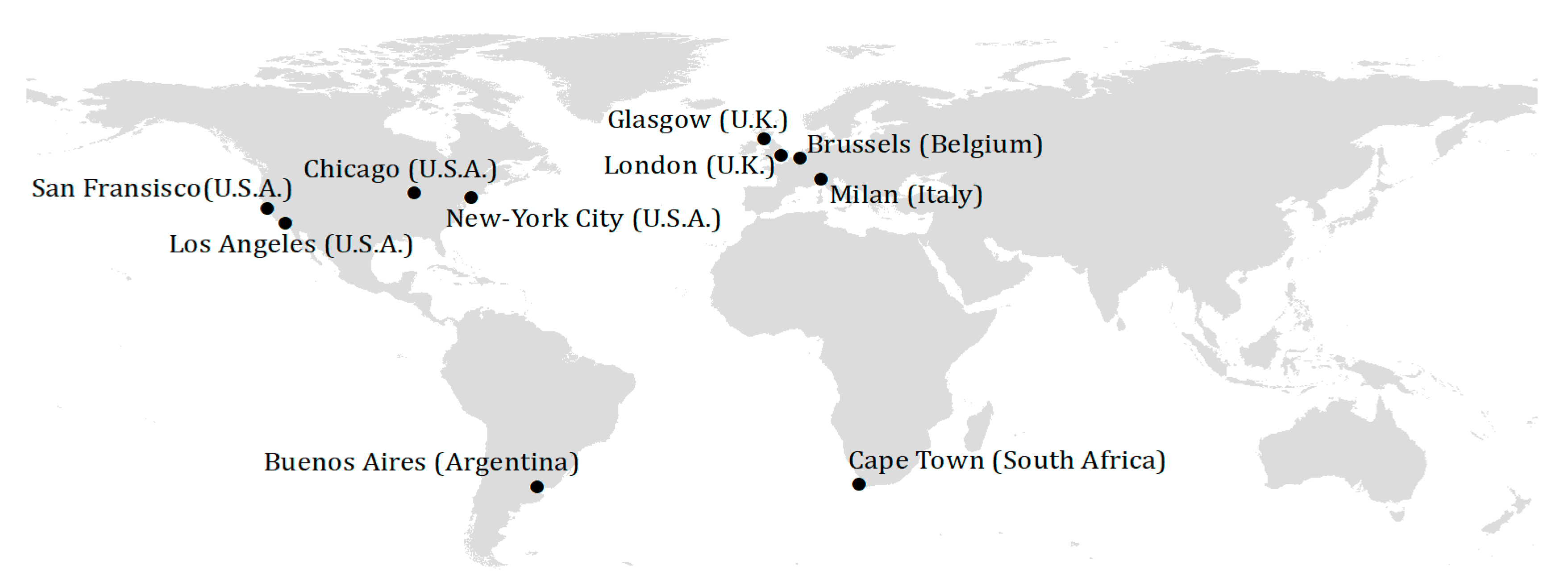
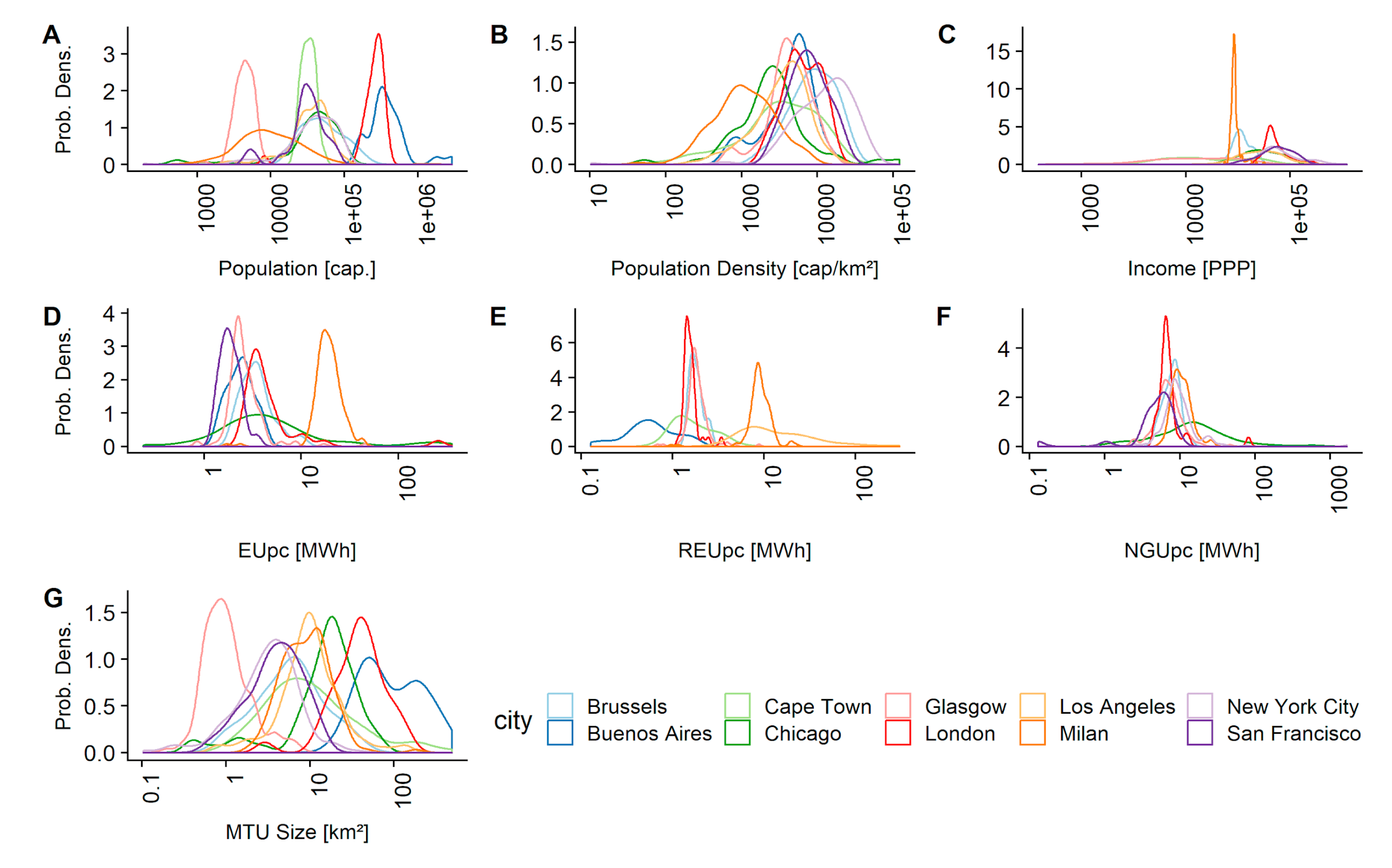
2.1. Presentation of the Case Studies and Data

The findings of this paper are based on data from ten cities located on four continents and in six countries, with different economic development stages, as well as in different climatic zones as illustrated in Figure 1, and most importantly, wide distribution in studied urban features. Cities were selected to reflect large variation of population sizes—from less than one to more than ten million inhabitants—widely distributed population densities of different orders of magnitude and displaying substantial difference in median income—from one to five. However, the selection of case studies was largely limited by the data availability at infra-urban scale. This last criterion has largely shaped the scope of the study and its limitation in cross-city analysis as explained and exemplified in the next sub-sections. Data sources varied from open database platforms, national and local statistical offices, grid operators, and scientific literature (for source of datasets, see Supplementary Material, Table S2). To measure the energy use of these cities, we used indicators focusing on different energy vectors (electricity and natural gas) and on different end uses (total use and residential use). Few cities have available data for all the combinations of energy vectors and end uses. Regarding the quality of data, it is also worth mentioning that, although all datasets used in this study come from a reputable source (i.e., metered by grid operator, emitted by regional statistic institutes), metadata are sometimes unclear. This is the case of “total electricity” and “total natural gas”, which in principle should include all electricity or natural gas usage on the corresponding territory, but it is unclear if this the case. We assumed in this study that it is the case, which may or may not affect the comparability between cities. Finally, the data used span from 2010 to 2014, which is a limitation to the comparability between cities, and no more recent data could be found.

Energy data were compared to three main urban indicators: population size, population density, and median income at purchasing power parity (PPP). The PPP median income used here is the median income of the city translated to USD and multiplied by the ratio of purchasing power of the USD and the currency of the country. This allows comparability of the purchasing power of citizens instead of the differences in the values of the currencies. For all the selected cities, data on additional urban indicators were available; however, these three were the indicators which were available for most of the cities and are relevant regarding energy use driver identification (e.g., [14,24,56,57,67]). For other indicators, the degree of overlap across the cities was too small to perform a meaningful analysis. Table S3 in Supplementary Material provides an account of the data encountered for each of the selected cities, such as other energy vectors and sectoral divisions.

2.1.1. Macroscale Data

The summary provided in

Table 1. Socioeconomic, demographic and energy data for the 10 selected global cities (N/A: Not available data, for sources of dataset, see Supplementary Material Table S2).

Indicators	Europe				North Am.				Africa	South Am.
	Milan	London	Brussels	Glasgow	N.-Y.C.	L.A.	San Francisco	Chicago	Cape Town	Buenos Aires
	Macroscale
Population [Millions cap.]	3.18	8.66	1.16	0.60	8.23	4.56	0.81	3.08	3.74	12.81
Area [km2]	1574	1572	161	172	775	1835	121	1477	2461	3209
HDD (15.5/15.5)	1840	1781	2080	2410	1958	306	754	2785	458	740
CDD (15.5/15.5)	918	349	362	105	1145	1413	439	986	1090	1423
Average income per household (PPP) [USD]	29,782	76,399	35,277	16,667	N/A	58,820	75,813	55,437	18,461	N/A
EU - Electricity use [GWh]	61,247	40,957	5004	1279	N/A	N/A	1412	11,610	N/A	34,170
EUpc - Electricity per capita [MWh/cap]	19.28	4.73	4.30	2.13	N/A	N/A	1.75	3.77	N/A	2.67
REU - Residential electricity use [GWh]	24,292	13,204	2226	1113	N/A	60,662	N/A	N/A	5060	10,921
REUpc - Resid. Elec. use per cap. [MWh/cap]	7.65	1.52	1.91	1.85	N/A	13.30	N/A	N/A	1.35	0.85
NGU- Natural gas use [GWh]	N/A	59,102	9732	1807	81,002	N/A	4355	31,792	N/A	N/A
NGUpc - Natural gas per capita [MWh/cap]	N/A	6.82	8.36	3.00	9.84	N/A	5.41	10.32	N/A	N/A
	Microscale
MTU boundaries	Munici-palities	Boroughs	Munici-palities	Interme-diate zones	Zip codes	Zip codes	Zip codes	Zip codes	Wards	Partidos
Number of MTUs	134	33	19	133	236	123	27	68	82	25
Average size of MTUs [km2]	12	48	8	1	3	15	4	22	30	128

gives an overview of the case studies and alludes to some of the challenges encountered in the data collection process. The main one is the unavailability of certain data (e.g., electricity use for New York City), another one is the variation in the boundaries definition for each city: some data cover geographical regions which include the city sprawl entirely, sometime encompassing some non-urban area (e.g., Cape Town), while others are limited to a highly urbanized core (e.g., Brussels). These differences can limit the comparability between case studies. For example, considering that the density of population is significantly higher in the city centres than in suburbs [34], excluding the suburbs of cities or including territory beyond cities may significantly alter some indicators used in this study (e.g., per capita energy use or density). However, these are inherent limitations of the type of research conducted here, using data collected or provided by local administrations within boundaries that make sense to them locally.

Overall the ten cities vary greatly in their consumption patterns on a macroscale. Milan is the largest consumer of electricity in our dataset. Moreover, Milan with 19.28 MWh/cap is also the largest consumer of electricity per capita and is ten times bigger than the figures of San Francisco (1.8 MWh/cap). Los Angeles has the highest residential electricity use per capita (13.30 MWh/cap). Chicago, being the third largest consumer of natural gas, is the largest consumer of natural gas per capita in our dataset (10.32 MWh/cap).

2.1.2. Microscale Data

Considering sub-city level data, one of the issues with regards to the comparability, both within and between cities, comes from the various definitions of micro territorial units (MTUs) found across cities (see “MTU boundaries” in Table 1). MTUs usually follow administrative spatial divisions (e.g., municipalities) which can result in large disparities in sizes and land use coverages. One of the most extreme cases is found in Brussels’ MTUs, defined by municipalities, where Saint-Josse-ten-Noode and Ville de Bruxelles have areas of respectively 1.14 (<1% of the city’s area) and 32.61 km² (~20% of the city’s area). The latter covers urban fabric and land use that are very heterogeneous, from the dense city centre to the northern suburb of the city, while the former, due to its small size, covers a quite homogeneous urban fabric. Therefore, the type of urban fabric and land-use averaged in the indicators are of different levels of homogeneity, affecting in turn the comparability of indicators within the same city. Additionally, data on urban indicators and on energy use were not always easy to find at the same spatial unit, which implied a limited number of variables in the analysis. Furthermore, it was not always possible to find energy-use data both by sources (electricity and natural gas) and by final uses (residential and total). This implies that the relation found in the analysis could not be established for all indicators (energies by sources, density of population, population, and income) for all cities. This type of limitation related to data availability are inherent of this type of research and has limited the reach of our analysis. Finally, some datasets were incomplete or censored by the data provider, displaying values of “0” for specific MTUs. Theses MTUs were disregarded from the study.

Figure 2 illustrates the (kernel estimation of) probability density distribution for the studied variables for each city, at microscale in a logarithmic scale. These continuous functions of probability for each city and indicator are approximated from the finite numbers of observations (with n between 19 and 236) and provide an easy way to display the relative likelihood of values for the indicators for each city.

Figure 2A,G give the probability density function of the population and area of MTU across cities. These distributions are displayed in absolute values and give a sense of how large the MTU and scale of observation are within and across cities. Regarding population (Figure 2A), with the exception of Milan, which spans across three orders of magnitude, three groups of distribution can be drawn: first, Glasgow with the smallest mean and overall values of MTU’s population (between one and one thousand people); then London and Buenos Aires with the largest values and maximum mode well above a hundred thousand people and some MTUs over a million people; and finally, the remaining six cities with their (maximum) mode around the same values, between 10 thousand and 100 thousand people. Regarding uniformity of the population distribution, Glasgow, Cape Town and London have very little skewness and small spread around their mode, displaying a rather uniform population size across MTU’s, while having each largely different mean population sizes distributed across three orders of magnitude. Milan, however, displays the most uniform distribution of population of all cities. The remaining cities, Brussels, Los Angeles, New-York City, Buenos Aires, Chicago, and San Francisco span across two or less orders of magnitude. Figure 2G gives an overview of the distribution of MTU sizes and scales of observation. The major observation that can be drawn from it is that the case studies span across vastly different territorial scales. Glasgow and Buenos Aires have their respective means and modes around 1 and 100 km², and all other cities are well distributed between those extremes. In terms of population density, Figure 2B data trends show substantially more overlapping in their distributions. As illustrated, most cities exhibit relatively similar population densities across their MTUs. These similarities in distributions are a remarkable result, all cities having vastly different metrics: area, population size, MTU sizes, and, MTU divisions. In some—notably Milan, Cape Town, and New York City—the distribution is more widely spread. This is mainly due to the different levels of sprawling in these cities, but it can also be partially attributed to the variety of cities’ boundary definitions. Lastly, Figure 2C displays the median income (PPP) distribution across MTUs. While the mean of the median income at purchasing power parity is relatively similar across cities, the distributions are characterized by very long tails, as is illustrated in Figure 2C. Only in the case of Milan, most MTUs appear to have a similar median income.

In the case of total electricity use per capita displayed in Figure 2D, the MTUs of all cities appear to have overlapping (probability density) distributions with most cities being clustered around a similar mode and mean (except Milan), and exhibiting similar standard deviations (except Chicago). Chicago displays a very large standard deviation for this indicator, although this city is not an outlier in terms of population, population density or MTU size. Milan appears to be an outlier by showing significantly higher median values than the other cities. After further investigation, no simple explanation could be found as to why Milan is an outlier. The residential electricity use per capita (REUpc) displayed in Figure 2E exhibits the greatest degree of disparity of all distributions in terms of mode, means and standard deviation. Three groupings can be made. London, Glasgow, and Brussels have a similar mean with very little standard deviation whereas Buenos Aires, Cape Town, and Los Angeles exhibit larger disparities between MTUs and means of distributions. Finally, Milan displays larger mean values and quite low disparity between MTU. Milan and Los Angeles have a similar residential energy use mean. Natural gas use (NGU) per capita distributions show a remarkable overlapping in the distributions between cities as displayed in Figure 2F. All cities exhibit a similar mean natural gas use per capita, with some cities displaying quite different standard deviations (i.e., Chicago and London). In Chicago however, the distribution is more homogeneously distributed across the use range than in the case of the other cities.

2.2. Method

In order to determine whether trends, that can be identified by analysing data at city level, also hold true when looking at data on a smaller spatial scale—such as the individual MTU—an exploratory analysis was conducted in which a linear regression was performed between the variables measuring per capita energy use and the selected urban indicators. The linear regressions on log-transformed urban indicators have been successfully used in urban scaling studies [14,29,30,32,34,39,40,44,68,69] in order to determine relations between urban indicators. Usually they have been used to determine how a certain property, captured by an indicator, scales with cities’ size. Our method extends these linear relations to other parameters than city population—namely, density and income, usually associated with urban energy use [14,24,56,57]—examining linear relations beyond sub- or super-linearity. Our method also extends relation identification to other scales of observations than city-scale—namely, micro-territorial units. This, in turn, provides ways to investigate if there is evidence of scale dependency of urban energy drivers.

These linear regressions are performed in three different configurations: (1) regressions “at the city level”, in accordance to previous urban scaling studies and with each data point being an aggregate indicator for the entire city; (2) by looking at data “at MTU level” where all MTUs are analysed at once regardless of the city they belong to; and (3) by looking at data at the level of the MTUs for each city individually where each city has its own regression. In the first configuration, regression at city-scale identifies the relations in the same method and framework as existing scaling law studies but with an extension to smaller cities and other indicators. In order to have a greater data set for the investigation at city scale, the data that are available in the paper by Kennedy et al. on material and energy metabolism of megacities [13] have been added to have more observations at city scale, with the exception of four cities (Buenos Aires, London, Los Angeles, New York), which were already present in the case studies. However, additional data could not be found for median income at city level in this literature, limiting the number of data points at city scale for this indicator. In the second configuration, similarly to the first one, cities are also examined to see if they share similar behaviours, but by looking at infra urban territories instead of the average indicator on the whole city. This provides a first examination of whether drivers found at city scale can be extended to lower scales, suggesting scale independency for these energy use drivers. To support scale independency, the slopes and predictive power at macro and micro scales should be similar. Finally, with the third configuration, which looks at relations for cities individually, it is possible to review whether or not cities have similar trends to one another, and if those relations corroborate the ones found in the other two configurations. This analysis allows us to explore whether the urban indicators that we are considering in this paper—population size, population density, and median income—act as drivers of intensity of urban energy use, and whether the relationship is different when looking at data at the aggregate level and at each city individually.

Finally, the originality of the approach does not reside in the technicality of univariate linear regression (via least-squares approach) in logarithmic space to determine drivers of urban feature, as it has been reviewed and successfully used in numerous previous studies [14,29,30,32,34,39,40,44,68,69]. However, the contribution lies in comparing relationship between energy use and urban indicators both at city-scale and sub-city micro-territories for a significant number of cities worldwide.

3. Results

Following the main objectives of this article, the results are subdivided in sections for each urban feature analysed (population size, population density, and median income), where the three sets of configurations explained above are investigated and compared to one another.

3.1. Energy Use and Population Size

Figure 3 provides a visualization of the regressions performed in the three above-mentioned configurations for the three intensity of energy use indicators and population size.

Table 2. Performance measures of population regression models.

	EUpc vs. Pop.			REUpc vs. Pop.			NGUpc vs. Pop.
	n	slope (β)	r2	n	slope (β)	r2	n	slope (β)	r2
City-scale	30	−0.09	0.02	26	−0.35	0.3 **	26	−0.53	0.33 **
MTU aggreg.	425	−0.14	0.05 ***	535	−0.13	0.04 ***	580	−0.08	0.03 ***
Brussels	19	0.14	0.07	19	0.07	0.14	19	0.09	0.06
Milan	134	−0.02	0.01	134	−0.09	0.09 ***	134	−0.06	0.04 *
Cape Town		NA	NA	82	−0.24	0.02		NA	NA
Buenos Aires	25	0.01	0	25	0.07	0.03		NA	NA
Chicago	58	−0.97	0.85 ***		NA	NA	58	−0.79	0.71 ***
London	33	−1.04	0.76 ***	33	−0.16	0.64 ***	33	−0.63	0.8 ***
San Francisco	23	−0.12	0.24 *		NA	NA	23	0.43	0.34 **
Los Angeles		NA	NA	109	−1.1	0.78 ***		NA	NA
Glasgow	133	−0.27	0.06 **	133	−0.29	0.23 ***	133	−0.15	0.02
New York City		NA	NA		NA	NA	180	−0.3	0.18 ***

p-values: *** for p ≤ 0.001; ** for p ≤ 0.01; * for p ≤ 0.05.

gives a summary of some measures of performance of these regressions. When looking at the relationship between population and the variables capturing intensity of energy use (per capita residential electricity use, per capita total electricity use, per capita natural gas use) at the macro level, the correlations have some significance. When it comes to total electricity use per capita (Figure 3A), the p-values are too weak to assess significant correlation. However, for natural gas use per capita (Figure 3G), and for the residential electricity use per capita (Figure 3D), the relation seems to be more significant but rather weak (r² ~ 0.3 & p ≤ 0.05 in both cases). This finding implies that at a macro scale it appears that cities with a higher population consume relatively less energy per capita.

At the level of the MTUs aggregated for all cities simultaneously (Figure 3B,E,H), the correlations seem to be more significant than at city scale. There is a dominant negative correlation between population size and per capita energy use for all energy indicators, although in the case of natural gas use, it appears to have less influence, as is illustrated in Figure 3H and Table 2. This indicates the same direction of dominant relation if compared to the correlations at the city level. However, at the MTU scale, much less of the variance (see Table 2) of residential electricity and natural gas use could be attributed to a change in population size. It is also important to mention that the p-value is affected by the sample size, with smaller p-value for larger samples. This could partially explain why correlations of aggregated MTU across cities (with n = 425 to 580) exhibit significantly lower p-value than of city-scale (with n = 26 to 30). However, the sample size effect can be considered low for R between 0.17 and 0.22 [70] for the all regressions of aggregated MTU.

At the MTU level for individual cities, which are depicted in Figure 3C,F,I, the picture is more contrasted. For total electricity use per capita (Figure 3C), London and Chicago exhibit a remarkably strong negative correlation (slopes of β = −1.04 and −0.97 respectively) with population size with a very low p-value (both being under 0.001) and high r² values (0.76 and 0.85 respectively). San Francisco also displays a significant correlation with population (p ≤ 0.05, r² = 0.24). The statistical power of the regression for Glasgow is not strong enough to determine a relation, even with its low p-value (p < 0.01, r² = 0.06). Brussels, Milan and Buenos Aires exhibit almost no meaningful correlation (p > 0.05). For this energy indicator, cities either have non-significant correlations or display a negative one following the same trend as Figure 3B. It seems that the validity of the correlation found across all cities at MTU scale could be questioned (Figure 3B) or even interpreted as a Yule–Simpson [71] effect given that not all cities, taken individually, follow the same trends. Rather, there is a great variability of responses from each city concerning the population size, while some have a very strong correlation (namely Chicago and London).

When looking at residential electricity use per capita (Figure 3F), the majority of cities would exhibit a negative correlation when they are significant. Los Angeles and London display a strong correlation with a large percentage of variance that could be attributed to population variation (both with p ≤ 0.001 with r² = 0.78, and β = −1.1 and r² = 0.64, and β = −0.16 resp.). Glasgow displays a weaker (r² = 0.23, and β = −0.29) but significant correlation as well, while the statistical power of the regression for Milan is too low to be relevant. The other cities (Brussels, Cape Town, and Buenos Aires) exhibit non-significant correlations. All significant regressions for residential electricity use seem to follow the same trend, but for cities individually, the correlation seems to be stronger than in the other configurations.

For natural gas use per capita (Figure 3I), Chicago, London and San Francisco exhibit strong to moderate correlations (r² = 0.71, 0.8, and 0.34 resp.). However, San Francisco seems to have the opposite trend (β = +0.43) than the other two cities (β = −0.79, −0.63). New York exhibits a weak but significant correlation (r² = 0.18, β = −0.3). Other cities do not have significant trends.

Overall, it appears that the majority of cities seem to share the same negative trend when correlations are significant, and with the exception of San Francisco for natural gas use per capita. When significant, the correlations for cities individually (Figure 3C,F,I) seem to have better predicting power while presenting variations in trends. Indeed, the importance of this driver varies from city to city with both r² and β ranging from nil to very strong. At city scale, as displayed on Figure 3D,G, the population does not appear to be a strong driver at a city scale (r² ≤ 0.33) when significant, at least not with the linear model used in this analysis, and it does not seem to affect the intensity of electricity use (Figure 3A). This driver is therefore inconsistent and could not be generalized. Furthermore, the scaling of those energy indicators with the population size, both at city and MTU scales, is not exhibited in these results. In extension to this analysis, it is not possible to conclude that bigger (or more populated) cities are more efficient, but rather that each city appears to respond very differently to population size, or even that population could not be considered as a driver in some cases.

3.2. Energy Use and Population Density

In this section the correlations of the population density with the three indicators of the intensity of energy use are examined. Figure 4 displays the regressions in the three configurations while

Table 3. Performance measures of population density regression models.

	EUpc vs. Density			REUpc vs. Density			NGUpc vs. Density
	n	slope (β)	r2	n	slope (β)	r2	n	slope (β)	r2
City-scale	28	−0.15	0.06	26	−0.09	0.03	24	−0.31	0.11
MTU aggreg.	425	−0.49	0.33 ***	535	−0.37	0.2 ***	580	−0.17	0.13 ***
Brussels	19	−0.06	0.02	19	−0.06	0.13	19	−0.18	0.3
Milan	134	−0.05	0.02	134	−0.1	0.09 ***	134	−0.09	0.09 ***
Cape Town		NA	NA	82	−0.13	0.23 ***		NA	NA
Buenos Aires	25	0.09	0.09	25	0.06	0.04		NA	NA
Chicago	58	−0.42	0.17 ***		NA	NA	58	−0.65	0.52 ***
London	33	−0.03	0	33	−0.06	0.07	33	−0.19	0.05
San Francisco	23	−0.02	0.01		NA	NA	23	0.29	0.12
Los Angeles		NA	NA	109	−0.61	0.35 ***		NA	NA
Glasgow	133	−0.06	0.01	133	−0.06	0.04 *	133	−0.12	0.05 *
New York City		NA	NA		NA	NA	180	−0.27	0.21 ***

p-values: *** for p ≤ 0.001; * for p ≤ 0.05.

gives the performance of the regressions.

It appears that the regressions for this driver are not statistically significant at city scale. At this scale, Figure 4A,D,G and Table 3 show that all three regressions have low coefficients of determination (r² = 0.06, 0.03, and 0.11, respectively) and too high p-values to be considered relevant (p ≥ 0.05). However, even if not significant, all three trends seem to display more of a negative impact of density increase on the intensity of energy use. These results at city scale (Figure 4A,D,G) are surprising and do not corroborate with the literature of driver of megacities energy use [14] where energy use per capita and population density seem to correlate (r² = 0.74) following a power-law (β = −0.75). This can be explained as this literature takes into account only megacities and investigates only the total energy use per capita. Therefore, it appears that, when extending the sample to smaller cities and looking at individual energy indicators, those power-laws do not hold.

When looking at the data at the level of the individual MTUs across all cities, the negative correlations between population density and energy use appear to be significant (p < 0.05) and encompass all the energy use indicators, as is illustrated in Figure 4B,E,H. Again, the density of population seems to have a negative relation with all energy indicators. However, these correlations are moderate and do not explain much of the variation of any energy indicator (with r² = 0.33, 0.2, and 0.13 respectively). When looking at data for each city individually (Figure 4C,F,I), the relations are clear and significant for few cities. For the per capita electricity use, almost none of the regressions are meaningful, with only Chicago having a weak (r² = 0.17) but statistically significant correlation (p < 0.001). For the residential electricity use, Los Angeles and Cape Town (r² = 0.35, and 0.23 resp. and β = −0.61, and −0.13 resp.) display meaningful relations. In case of natural gas use per capita, Chicago and New York City display statistically significant correlations (r² = 0.52, and 0.21 with β = −0.65, and −0.27 respectively). For all other non-significant relations, the direction of the slope stays substantially unchanged between cities.

Overall, it appears that density is a consistent driver of intensity of energy use only when looking at MTU scale across cities. In other cases, the driving power of this urban feature seems to be variable from cities to cities, and non-existent at city scale. This last result does not corroborate with previous studies made for megacities.

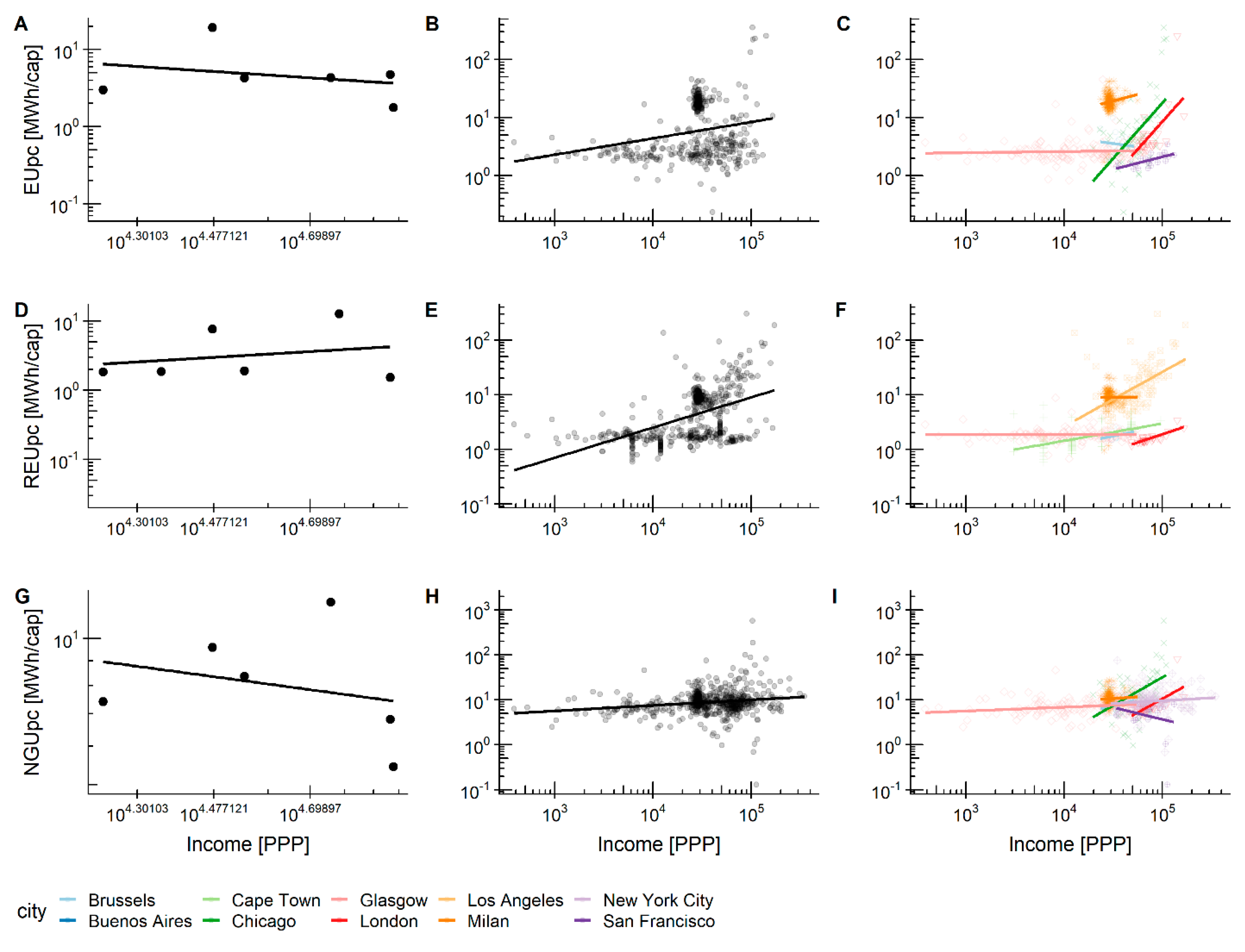
3.3. Energy Use and Median Income (PPP)

In this section the regressions between energy use and median income are investigated and displayed in Figure 5 and

Table 4. Performance measures of median income (PPP) regression models.

	EUpc vs. Income			REUpc vs. Income			NGUpc vs. Income
	n	slope (β)	r2	n	slope (β)	r2	n	slope (β)	r2
City-scale	6	−0.31	0.08	6	0.33	0.07	6	−0.1	0.07
MTU aggreg.	400	0.25	0.06 ***	510	0.45	0.23 ***	579	0.12	0.04 ***
Brussels	19	−0.21	0.02	19	0.23	0.17	19	0.46	0.17
Milan	134	0.4	0.02	134	−0.02	0	134	0.14	0
Cape Town		NA	NA	82	0.19	0.26 ***		NA	NA
Buenos Aires		NA	NA		NA	NA		NA	NA
Chicago	58	1.67	0.34 ***		NA	NA	58	1.18	0.22 ***
London	33	1.72	0.38 ***	33	0.39	0.69 ***	33	1.12	0.47 ***
San Francisco	23	0.28	0.42 ***		NA	NA	23	−0.2	0.02
Los Angeles		NA	NA	109	0.93	0.27 ***		NA	NA
Glasgow	133	0.02	0	133	0	0	133	0.07	0.04 *
New York City		NA	NA		NA	NA	180	0.12	0.01

p-values: *** for p ≤ 0.001; * for p ≤ 0.05.

. At city scale, as shown in Figure 5A,D,G, the number of data points for the median income (PPP) is lower than for the other urban features analysed here because no additional data could be found in the same literature. The small number of data points limits the conclusion to whether the median income is a potential driver of energy use at city scale. However, the correlations between income and energy seem to be quite spurious when looking at regressions at the city level (Figure 5A,D,G), with none of the relations being significant (p ≥ 0.05 and r² ≤ 0.1). When looking at data at the MTU level across cities (Figure 5B,E,H), it seems that only the residential electricity per capita is (moderately) positively correlated with the median income (p ≤ 0.05, r = 0.23 and β = 0.45), the intensity of electricity and natural gas use being almost unaffected. Moreover, the relationships look very discontinuous for electricity use, and residential electricity use, and they do not seem to follow a linear pattern. The natural gas use however seems to follow a more linear but very weak trend.

When looking at individual cities (Figure 5C,F,I), there are significant relations (p ≤ 0.001) showing positive correlation with median income. In particular, the electricity use of Chicago, London, and San Francisco are moderately correlated (r² = 0.34, 0.38, 0.42, respectively) with their median income. Cape Town, Los Angeles and London’s median incomes correlate (moderately and strongly) with residential energy use (r² = 0.26, 0.27, 0.69, respectively). Finally, the regressions for natural gas use per capita are significant only for Chicago and London (r² = 0.22, and 0.47 respectively). It is also interesting to see that Brussels, Milan, and Glasgow do not display any correlation for median income with any of the energy use indicators, while London displays correlations for all energy use indicators and San Francisco does correlate with energy use per capita but does not correlate with natural gas use per capita.

Overall, when correlations are significant between the median income and the three indicators of energy use, the trends show positive relations. However, these relations only exist at MTU scale, and more importantly, only strongly for some cities. This shows again that cities respond differently to the same urban features, and differently for each energy indicator.

4. Discussion

Some major findings can be highlighted from this investigation and subsequent results. First, the scaling law of the intensity of energy consumption [14] is not corroborated for cities other than megacities and for other energy use metrics. Indeed, we found only two potentially meaningful relations at city scale: the population size seems to correlate negatively with both residential electricity and natural gas use per capita (see “Energy use and population size” section). However, only a fraction of the variation in those energy intensity indicators can be predicted by population size with r² ~ 0.3 in both cases. The density of population was found not to be a good predictor of any of the three indicators of energy use intensity, contrary to what has been found in previous study [14]. The median income (PPP), while being sometimes highlighted as a driver or energy consumption (e.g., [9,10] and, sometimes in larger scales like nation-wise [57]) appears to not be a good predictor of energy use intensity. Regarding power-law across cities at MTU level, two out of nine relations are relevant: the density of population with the energy use per capita, and the median income (PPP) with the residential energy use, although only a small portion of variance is predicted based on these urban features (r² ~ 0.33, and 0.23 resp.). Despite a large sample (400 to 579 observations) no shared behaviour could be found otherwise.

Secondly, while there is no major contradiction in trends across scales (city scale or MTU scale) and scopes (across cities or city by city), the exploratory analysis has shown that the relationship between urban indicators and urban energy use is not in all cases scale invariant, showing that intensity of energy use could be an intensive feature of urban systems. Indeed, correlations observed at the city level substantially change at the MTU level, especially when studied for each individual city. When looking at data aggregated at the city level, a tendency towards a negative correlation between population densities and energy use can be observed, this trend could not be observed systematically when looking at data for the individual cities at the MTU level. This echoes previous findings which state that the relation between density of urban fabric and residential energy use remains unclear [72], and that density as a driver is less relevant at infra-urban scale where other factors come into play [13,73]. In the case of the relationship between income and urban energy use, when looking at data aggregated at the city level, there seemed to be a roughly linearly increasing relationship between the two variables. However, when looking at data at the MTU level, some cities exhibit either nil correlations or strong positive ones, which corroborates previous findings at infra-urban scale which exhibit weak correlation between those variables [13]. A significant number of deviations from the city level correlation were also observed in the relations between population size and urban energy use.

Lastly, when a relation exists between one of the urban features analysed and intensity of energy use indicators, the regressions of individual cities usually give better predictions than predictions across cities. However, not all cities respond to the same drivers, with some being unaffected by population, density, or income variations, while others vary almost linearly with them.

This investigation offers several points of discussion subsequent to findings. Firstly, previously found city-scale power-laws of intensity of energy use do not seem to hold when taking into account smaller cities and looking at indicators of intensity of energy use other than total energy use per capita. This relativizes and gives new perspectives to the previous researches on scaling laws of urban energy use [13,14] for megacities. Indeed, none of the evidence and data collected for this study contradicts previous research: the overall tendencies are that intensity of energy consumption increases with income and decreases with population density and population size. However, no evidence clearly supports previous findings either. On the contrary, the relations seem to be more complex when extending the case studies. In order to take other cities into account, better indicators of the intensity of energy use or more complex relations might be necessary. Future research should therefore investigate how those relations could be extended to more cities, using more complex regression methods, larger sets of case studies and features.

Secondly, the regressions across cities at MTU scale correlate, with statistical significance, for all urban indicators and intensity of energy use indicators, suggesting the existence of power-laws for this scale. However, this result needs to be put in perspective since the slopes and r² for city-wise regressions are vastly different and do not corroborate this result. For these reasons, the power-laws at MTU scale across cities, might by interpreted as Yule–Simpson effect. Therefore, these results should be considered as inconclusive.

Thirdly, the relationships between different urban indicators and variables measuring urban energy use are not the same when looking at data aggregated at the city level, or data at the level of individual MTUs. This inconsistency of drivers points towards a scale dependency of energy drivers. The intensity of energy use might be an intensive feature of urban system, and its value will change depending on the scale of observation. This has implications for both identification of energy drivers in future researches and policy making. These “scale effects” should therefore be considered for the samples that are observed or the territory that are regulated. More importantly, this raises a more fundamental question: if urban features act differently on the intensity of urban consumption depending on the scale of observation, how do these drivers interact with each other? Future research should investigate this further to better define the relation between drivers and the scale of observations. However, with present results, the scale-dependency of the drivers of energy use suggests that the urban planning regulation may need to be designed to reflect the different behaviour at different scale, and therefore should propose multi-scale strategies to tackle energy-use reduction at all potential levels.

Fourthly, city-scale regressions have lower predictive power than city-wise regressions. More specifically, the drivers that are statistically significant are usually present for cities individually. Furthermore, this study also shows that, when looking at data at the level of the MTUs for each city individually, there is a great heterogeneity across the different cities regarding the nature of the relationship between urban indicators and per capita energy use. This result weights in favour of city-specific power-laws and drivers and indicates that there are factors that differ across cities, which confounds this relationship. The fact that at infra-urban scale drivers of energy use seem to be city-specific should encourage local decision makers to explore and determine the specific features of their city where actions can be made to seek best result, as two different cities may respond very differently to the same driver. It points towards the importance of local drivers, which are not taken into account when looking at data at the aggregate level. Such observations expose the limitations of analysing cities as homogenous wholes. If we want to make cities more sustainable, and act on their energy consumption, it is important to take into consideration such local-level drivers.

Like most studies relying on large amounts of data, this study is also subjected to some important limitations regarding the comparability of the data across different cities. One of these limitations is the way cities are bounded. The definitions of a “city” in the case studies investigated here depend on the administrative boundaries which may or may not include the entire continuous urban fabric of the cities. In some cases (Milan for example), the boundaries of the city include all of the extensions and suburbs of the city; while in other cases, some of the urban fabric is left outside of the administrative boundaries (Brussels for example). The differences in periods of time between cities in our dataset, ranging from 2010 to 2014, is also a factor limiting the comparability. By doing so we assume that relationships between variables, expressed in the power-law regression performed, are constant over the four years of our dataset. We consider that this assumption can be made as the large demographical, technological, and behavioural changes needed to impact the relationships between these variables are unlikely to happen over a 4-year period. However, this limitation is common in this type of study and demonstrates again that it is crucial for researchers and city planners that urban energy data are annually produced.

Another important element is that the way in which MTUs are delimited in different cities varies largely. These variations exist both across cities and within individual cities. This results in the MTUs corresponding to different spatial units, differing in sizes and characteristics. For instance, Glasgow as a city is roughly the same size as some of Buenos Aires’ MTUs, and MTUs of Brussels cover anything between 1% and 20% of the area of the city. Another limitation is that the purpose of the final energy use is not clearly known and can vary a lot from city to city. For instance, in some cities, natural gas is used for heating, domestic hot water, and cooking, whilst in other cities, the latter two are provided by electricity. This may affect the comparability between cities since certain energy vectors might cover different uses which in turn might be driven by other sets of drivers. As mentioned in the literature [24], larger incomes can correlate with larger housing and therefore heating demands which might be related to different energy vectors depending on the city that is analysed. Furthermore, the number of sectors considered as final users of energy also varies across the different cities, where some cities name three—residential, commercial, and industrial—and others up to five. This shows that future research should look in more detail into the end-purpose of energy spending, rather than simply by sectors or vectors. It should also be recommended to include urban indicators beyond the ones used for this study—population size, population density, and median income—in order to explore other potential drivers of urban energy consumption, notably at a local scale.

5. Conclusions

In this study we have examined 10 cities worldwide, across three energy use intensity indicators (electricity use per capita, natural gas use per capita, residential electricity use per capita) and three urban features (population, population density and PPP median income). The power-law relationship between energy use indicators and urban feature are examined at city scale and at sub-city scale (micro-territorial unit, MTU). The main goals of the study were: (1) to investigate if power-laws relationship could be found for smaller cities (in population) than previous studies and disaggregated energy flows; (2) to see if such power-law could be extended to sub-city scale suggesting scale independency of these drivers; (3) to investigate if cities observed individually would exhibit comparable power-law when examined at MTU scale. This investigation has shown that: (1) it is unlikely that power-law found in previous study [14] could be extended to smaller cities and disaggregated energy flows; (2) there is a scale dependency of drivers regarding the intensity of urban energy use; and (3) that there is heterogeneity regarding the nature of the relationships found city-wise across the different cities. These results have several limitations, mainly related to various definitions of MTU and energy indicators across cities. However, the presented findings show some of the limitations of considering cities as homogeneous wholes. Instead, local drivers and local context should be taken into greater consideration in policy making in order to more effectively assist cities into their sustainable transitions. Future research should explicitly take into account the scale dependency of energy use drivers and should seek to provide multiscale analysis and modelling of urban systems.

References

1. Seto, K.C.; Dhakal, S.; Bigio, A.; Blanco, H.; Delgado, G.C.; Dewar, D.; Huang, L.; Inaba, A.; Kansal, A.; Lwasa, S.; et al. Human Settlements, Infrastructure and Spatial Planning. In Climate Change 2014: Mitigation of Climate Change. Contribution of Working Group III to the Fifth Assessment Report of the Intergovernmental Panel on Climate Change; Edenhofer, O., Pichs-Madruga, R., Sokona, Y., Farahani, E., Kadner, S., Seyboth, K., Adler, A., Baum, I., Brunner, S., Eickemeier, P., et al., Eds.; Cambridge University Press: Cambridge, UK, 2014. [Google Scholar]
2. ICLEI; UNEP; UN-Habitat. Sustainable Urban Energy Planning. A Handbook for Cities and Towns in Developing Countries; UN-Habitat: Nairobi, Kenya, 2009. [Google Scholar]
3. UN DESA. World Urbanization Prospects: The 2014 Revision, Highlights; United Nations Department of Economic and Social Affairs Population Division: New York, NY, USA, 2014. [Google Scholar]
4. Grimm, N.B.; Faeth, S.H.; Golubiewski, N.E.; Redman, C.L.; Wu, J.; Bai, X.; Briggs, J.M. Global change and the ecology of cities. Science 2008, 319, 756–760. [Google Scholar] [CrossRef] [PubMed]
5. Bertoldi, P.; Piers de Raveschoot, R.; Paina, F.; Melica, G.; Gabrielaitiene, I.; Janssens-Maenhout, G.; Meijide Orive, A.; Iancu, A. How to Develop a Sustainable Energy Action Plan (SEAP) in the Eastern Partnership and Central Asian Cities; Scientific and Technical Research Reports: Luxembourg, 2014; ISBN 1831-9424. [Google Scholar]
6. Rockström, J.; Steffen, W.; Noone, K.; Persson, Å.; Chapin, F.S., III; Lambin, E.F.; Lenton, T.M.; Scheffer, M.; Folke, C.; Schellnhuber, H.J.; et al. A safe operating space for humanity. Nature 2009, 461, 472–475. [Google Scholar] [CrossRef] [PubMed]
7. Grubler, A.; Bai, X.; Buettner, T.; Dhakal, S.; Fisk, D.J.; Ichinose, T.; Keirstead, J.E.; Sammer, G.; Satterthwaite, D.; Schulz, N.B.; et al. Urban Energy Systems. In Global Energy Assessment—Toward a Sustainable Future; Cambridge University Press: Cambridge, UK; New York, NY, USA; The International Institute for Applied Systems Analysis: Laxenburg, Austria, 2012; Chapter 18; pp. 1307–1400. [Google Scholar]
8. Creutzig, F.; Baiocchi, G.; Bierkandt, R.; Pichler, P.P.; Seto, K.C. Global typology of urban energy use and potentials for an urbanization mitigation wedge. Proc. Natl. Acad. Sci. USA 2015, 112, 6283–6288. [Google Scholar] [CrossRef] [PubMed] [Green Version]
9. Štreimikienė, D. Residential energy consumption trends, main drivers and policies in Lithuania. Renew. Sustain. Energy Rev. 2014, 35, 285–293. [Google Scholar] [CrossRef]
10. Zachariadis, T.; Taibi, E. Exploring drivers of energy demand in Cyprus–Scenarios and policy options. Energy Policy 2015, 86, 166–175. [Google Scholar] [CrossRef]
11. Warren-Rhodes, K.; Koenig, A. Escalating Trends in the Urban Metabolism of Hong Kong: 1971–1997. AMBIO J. Hum. Environ. 2001, 30, 429–438. [Google Scholar] [CrossRef] [PubMed]
12. Newcombe, K. Energy use in Hong Kong: Part II, sector end-use analysis. Urban Ecol. 1975, 1, 285–309. [Google Scholar] [CrossRef]
13. Kennedy, C.A.; Stewart, I.; Facchini, A.; Cersosimo, I.; Mele, R.; Chen, B.; Uda, M.; Kansal, A.; Chiu, A.; Kim, K.G.; et al. Energy and material flows of megacities. Proc. Natl. Acad. Sci. USA 2015, 112, 5985–5990. [Google Scholar] [CrossRef] [PubMed] [Green Version]
14. Facchini, A.; Kennedy, C.; Stewart, I.; Mele, R. The energy metabolism of megacities. Appl. Energy 2017, 186, 86–95. [Google Scholar] [CrossRef]
15. Athanassiadis, A.; Bouillard, P. Contextualizing the Urban Metabolism of Brussels: Correlation of resource use with local factors. In Proceedings of the CISBAT 2013, International Conference, Cleantech for Smart Cities & Building from Nano to Urban Scale, EPFL-Lausanne, Lausanne, Switzerland, 4–6 September 2013. [Google Scholar]
16. Athanassiadis, A.; Christis, M.; Bouillard, P.; Vercalsteren, A.; Crawford, R.H.; Khan, A.Z. Comparing a territorial-based and a consumption-based approach to assess the local and global environmental performance of cities. J. Clean. Prod. 2016, 173, 112–123. [Google Scholar] [CrossRef]
17. Lenzen, M.; Dey, C.; Foran, B. Energy requirements of Sydney households. Ecol. Econ. 2004, 49, 375–399. [Google Scholar] [CrossRef]
18. Wiedenhofer, D.; Lenzen, M.; Steinberger, J.K. Energy requirements of consumption: Urban form, climatic and socio-economic factors, rebounds and their policy implications. Energy Policy 2013, 63, 696–707. [Google Scholar] [CrossRef]
19. Duvigneaud, P.; Denayer-De Smet, S. L’écosystème URBS: L’écosystème urbain bruxellois. In Productivité Biologique en Belgique; Duculot, É., Ed.; Éditions Duculot: Paris, France, 1977. [Google Scholar]
20. Wang, Q.; Li, R. Drivers for energy consumption: A comparative analysis of China and India. Renew. Sustain. Energy Rev. 2016, 62, 954–962. [Google Scholar] [CrossRef]
21. Shammin, M.R.; Herendeen, R.A.; Hanson, M.J.; Wilson, E.J.H. A multivariate analysis of the energy intensity of sprawl versus compact living in the U.S. for 2003. Ecol. Econ. 2010, 69, 2363–2373. [Google Scholar] [CrossRef]
22. Howard, B.; Parshall, L.; Thompson, J.; Hammer, S.; Dickinson, J.; Modi, V. Spatial distribution of urban building energy consumption by end use. Energy Build. 2012, 45, 141–151. [Google Scholar] [CrossRef]
23. Baynes, T.; Lenzen, M.; Steinberger, J.K.; Bai, X. Comparison of household consumption and regional production approaches to assess urban energy use and implications for policy. Energy Policy 2011, 39, 7298–7309. [Google Scholar] [CrossRef] [Green Version]
24. Pincetl, S.; Newell, J.P. Why data for a political-industrial ecology of cities? Geoforum 2017, 85, 381–391. [Google Scholar] [CrossRef]
25. Batty, M. Building a science of cities. Cities 2012, 29, S9–S16. [Google Scholar] [CrossRef] [Green Version]
26. McPhearson, T.; Pickett, S.T.A.; Grimm, N.B.; Niemelä, J.; Alberti, M.; Elmqvist, T.; Weber, C.; Haase, D.; Breuste, J.; Qureshi, S. Advancing Urban Ecology toward a Science of Cities. BioScience 2016, 66, 198–212. [Google Scholar] [CrossRef] [Green Version]
27. Youn, H.; Bettencourt, L.M.; Lobo, J.; Strumsky, D.; Samaniego, H.; West, G.B. Scaling and universality in urban economic diversification. J. R. Soc. Interface 2016, 13, 20150937. [Google Scholar] [CrossRef] [Green Version]
28. Yakubo, K.; Saijo, Y.; Korosak, D. Superlinear and sublinear urban scaling in geographical networks modeling cities. Phys. Rev. E Stat. Nonlinear Soft Matter Phys. 2014, 90, 022803. [Google Scholar] [CrossRef] [PubMed]
29. Um, J.; Son, S.-W.; Lee, S.-I.; Jeong, H.; Kimd, B.J. Scaling laws between population and facility densities. Proc. Natl. Acad. Sci. USA 2009, 106, 14236–14240. [Google Scholar] [CrossRef] [PubMed] [Green Version]
30. Samaniego, H.; Moses, M.E. Cities as organisms: Allometric scaling of urban road networks. J. Transp. Land Use 2008, 1, 21–39. [Google Scholar] [CrossRef]
31. Pan, W.; Ghoshal, G.; Krumme, C.; Cebrian, M.; Pentland, A. Urban characteristics attributable to density-driven tie formation. Nat. Commun. 2013, 4, 1961. [Google Scholar] [CrossRef] [PubMed] [Green Version]
32. Oliveira, E.A.; Andrade, J.S., Jr.; Makse, H.A. Large cities are less green. Sci. Rep. 2014, 4, 4235. [Google Scholar] [CrossRef] [PubMed] [Green Version]
33. Nomaler, O.; Frenken, K.; Heimeriks, G. On Scaling of Scientific Knowledge Production in U.S. Metropolitan Areas. PLoS ONE 2014, 9, e110805. [Google Scholar] [CrossRef] [PubMed]
34. Lemoy, R.; Caruso, G. Scaling evidence of the homothetic nature of cities. arXiv 2017, arXiv:1102.4101. [Google Scholar]
35. Gomez-Lievano, A.; Youn, H.; Bettencourt, L.M. The statistics of urban scaling and their connection to Zipf’s law. PLoS ONE 2012, 7, e40393. [Google Scholar] [CrossRef]
36. Gomez-Lievano, A.; Patterson-Lomba, O.; Hausmann, R. Explaining the prevalence, scaling and variance of urban phenomena. Nat. Hum. Behav. 2016, 1, 0012. [Google Scholar] [CrossRef] [Green Version]
37. Bettencourt, L.M.A.; Lobo, J.; Youn, H. The hypothesis of urban scaling: Formalization, implications and challenges. arXiv 2013, arXiv:1301.5919. [Google Scholar]
38. Bettencourt, L.M.; Lobo, J.; Strumsky, D.; West, G.B. Urban scaling and its deviations: Revealing the structure of wealth, innovation and crime across cities. PLoS ONE 2010, 5, e13541. [Google Scholar] [CrossRef] [PubMed]
39. Bettencourt, L.M.; Lobo, J.; Helbing, D.; Kuhnert, C.; West, G.B. Growth, innovation, scaling, and the pace of life in cities. Proc. Natl. Acad. Sci. USA 2007, 104, 7301–7306. [Google Scholar] [CrossRef] [PubMed] [Green Version]
40. Bettencourt, L.M.; Lobo, J. Urban scaling in Europe. J. R. Soc. Interface 2016, 13, 20160005. [Google Scholar] [CrossRef] [PubMed]
41. Bettencourt, L.M. The origins of scaling in cities. Science 2013, 340, 1438–1441. [Google Scholar] [CrossRef] [PubMed]
42. Batty, M. The New Science of Cities; MIT Press: Cambridge, MA, USA, 2013. [Google Scholar]
43. Batty, M. The Size, Scale, and Shape of Cities. Science 2008, 319, 769–771. [Google Scholar] [CrossRef] [PubMed] [Green Version]
44. Arbesman, S.; Christakis, N.A. Scaling of Prosocial Behavior in Cities. Physica A 2011, 390, 2155–2159. [Google Scholar] [CrossRef]
45. Alves, L.G.; Ribeiro, H.V.; Lenzi, E.K.; Mendes, R.S. Distance to the scaling law: A useful approach for unveiling relationships between crime and urban metrics. PLoS ONE 2013, 8, e69580. [Google Scholar] [CrossRef]
46. Pincetl, S.; Bunje, P.; Holmes, T. An expanded urban metabolism method: Toward a systems approach for assessing urban energy processes and causes. Landsc. Urban Plan. 2012, 107, 193–202. [Google Scholar] [CrossRef]
47. Batty, M. Urban Modeling. International Encyclopedia of Human Geography; Kitchin, R., Thrift, N., Eds.; Elsevier: Oxford, UK, 2009; pp. 51–58. [Google Scholar]
48. Bai, X.; McAllister, R.R.J.; Beaty, R.M.; Taylor, B. Urban policy and governance in a global environment: Complex systems, scale mismatches and public participation. Curr. Opin. Environ. Sustain. 2010, 2, 129–135. [Google Scholar] [CrossRef]
49. Bai, X.; Surveyer, A.; Elmqvist, T.; Gatzweiler, F.W.; Güneralp, B.; Parnell, S.; Prieur-Richard, A.-H.; Shrivastava, P.; Siri, J.G.; Stafford-Smith, M.; et al. Defining and advancing a systems approach for sustainable cities. Curr. Opin. Environ. Sustain. 2016, 23, 69–78. [Google Scholar] [CrossRef]
50. Bowden, N.; Payne, J.E. The causal relationship between U.S. energy consumption and real output: A disaggregated analysis. J. Policy Model. 2009, 31, 180–188. [Google Scholar] [CrossRef]
51. Gross, C. Explaining the (non-) causality between energy and economic growth in the U.S.—A multivariate sectoral analysis. Energy Econ. 2012, 34, 489–499. [Google Scholar] [CrossRef]
52. Hoch, I. Income and City Size. Urban Stud. 1972, 9, 299–328. [Google Scholar] [CrossRef]
53. Mansfield, E. City Size and Income. In National Bureau of Economic Research. Regional Income; Wealth, R.I., Ed.; NBER: New York, NY, USA, 1949; pp. 271–318. [Google Scholar]
54. Brelsford, C.; Lobo, J.; Hand, J.; Bettencourt, L.M.A. Heterogeneity and scale of sustainable development in cities. Proc. Natl. Acad. Sci. USA 2017, 114, 8963–8968. [Google Scholar] [CrossRef] [PubMed] [Green Version]
55. Sarkar, S.; Phibbs, P.; Simpson, R.; Wasnik, S. The scaling of income distribution in Australia: Possible relationships between urban allometry, city size, and economic inequality. Environ. Plan. B Urban Anal. City Sci. 2016, 45, 603–622. [Google Scholar] [CrossRef] [Green Version]
56. Asafu-Adjaye, J. The relationship between energy consumption, energy prices and economic growth: Time series evidence from Asian developing countries. Energy Econ. 2000, 22, 615–625. [Google Scholar] [CrossRef]
57. Halicioglu, F. An econometric study of CO2 emissions, energy consumption, income and foreign trade in Turkey. Energy Policy 2009, 37, 1156–1164. [Google Scholar] [CrossRef]
58. Masih, A.M.M.; Masih, R. Energy consumption, real income and temporal causality: Results from a multi-country study based on cointegration and error-correction modelling techniques. Energy Econ. 1996, 18, 165–183. [Google Scholar] [CrossRef]
59. Soytas, U.; Sari, R.; Ewing, B.T. Energy consumption, income, and carbon emissions in the United States. Ecol. Econ. 2007, 62, 482–489. [Google Scholar] [CrossRef]
60. Mindali, O.; Raveh, A.; Salomon, I. Urban density and energy consumption: A new look at old statistics. Transp. Res. Part A Policy Pract. 2004, 38, 143–162. [Google Scholar] [CrossRef]
61. Bettencourt, L.; West, G. A unified theory of urban living. Nature 2010, 467, 912–913. [Google Scholar] [CrossRef] [PubMed]
62. Pincetl, S.; Graham, R.; Murphy, S.; Sivaraman, D. Analysis of High-Resolution Utility Data for Understanding Energy Use in Urban Systems: The Case of Los Angeles, California. J. Ind. Ecol. 2016, 20, 166–178. [Google Scholar] [CrossRef]
63. Newman, P.W.G.; Kenworthy, J.R. Gasoline Consumption and Cities. J. Am. Plan. Assoc. 1989, 55, 24–37. [Google Scholar] [CrossRef]
64. Kennedy, C.; Steinberger, J.; Gasson, B.; Hansen, Y.; Hillman, T.; Havránek, M.; Pataki, D.; Phdungsilp, A.; Ramaswami, A.; Mendez, G.V. Greenhouse Gas Emissions from Global Cities. Environ. Sci. Technol. 2011, 45, 3816–3817. [Google Scholar] [CrossRef]
65. Athanassiadis, A.; Crawford, R.H.; Bouillard, P. Exploring the Relationship Between Melbourne’s Water Metabolism and Urban Characteristics. In Proceedings of the State of Australian Cities 2015, Gold Coast, Austrila, 9–11 December 2015. [Google Scholar]
66. Porse, E.; Derenski, J.; Gustafson, H.; Elizabeth, Z.; Pincetl, S. Structural, geographic, and social factors in urban building energy use: Analysis of aggregated account-level consumption data in a megacity. Energy Policy 2016, 96, 179–192. [Google Scholar] [CrossRef] [Green Version]
67. Huebner, G.M.; Shipworth, D. All about size?—The potential of downsizing in reducing energy demand. Appl. Energy 2017, 186, 226–233. [Google Scholar] [CrossRef]
68. Shalizi, C.R. Scaling and hierarchy in urban economies. arXiv 2011, arXiv:1102.4101. [Google Scholar]
69. Sarkar, S.; Phibbs, P.; Simpson, R.; Wasnik, S.N. The scaling of income inequality in cities. arXiv 2015, arXiv:1509.00959v1. [Google Scholar]
70. Sullivan, G.M.; Feinn, R. Using Effect Size-or Why the P Value Is Not Enough. J. Grad. Med. Educ. 2012, 4, 279–282. [Google Scholar] [CrossRef]
71. Blyth, C.R. On Simpson’s Paradox and the Sure-Thing Principle. J. Am. Stat. Assoc. 1972, 67, 364–366. [Google Scholar] [CrossRef]
72. Rickwood, P.; Glazebrook, G.; Searle, G. Urban Structure and Energy—A Review. Urban Policy Res. 2008, 26, 57–81. [Google Scholar] [CrossRef]
73. Echenique, M.H.; Hargreaves, A.J.; Mitchell, G.; Namdeo, A. Growing Cities Sustainably. J. Am. Plan. Assoc. 2012, 78, 121–137. [Google Scholar] [CrossRef]
Figure 1. Map of the 10 selected case studies.
Sustainability 11 03246 g001
Figure 2. Kernel estimations of the probability density function across micro territorial units (MTUs) for each city and for the following urban variables: (A) population; (B) population density; (C) median income at purchasing power parity; (D) electricity use per capita; (E) residential electricity use per capita; (F) natural gas use per capita; (G) areas of micro territorial units (MTUs).
Sustainability 11 03246 g002
Figure 3. Regressions of electricity use per capita, residential electricity use per capita and natural gas use per capita with population at city scale (A,D,G), MTU scale aggregated (B,E,H) and MTU scale per city (C,F,I). At city scale level (first column), solid black circles correspond to the data from our sample, whereas hollow white circles are drawn from literature on energy use in megacities [13] in order to achieve a relevant number of observations.
Sustainability 11 03246 g003
Figure 4. Regressions of population density with electricity use per capita, residential electricity use per capita and natural gas use per capita at city scale (A,D,G), MTU scale aggregated (B,E,H) and MTU scale per city (C,F,I). At city scale level (first column), solid black circles correspond to the data from our sample, whereas hollow white circles are drawn from literature on energy use in megacities [13] in order to achieve a relevant number of observations.
Sustainability 11 03246 g004
Figure 5. Regressions of median income (PPP) with electricity use per capita, residential electricity use per capita and natural gas use per capita at city scale (A,D,G), MTU scale aggregated (B,E,H) and MTU scale per city (C,F,I).
Sustainability 11 03246 g005