Flow–Vegetation Interaction in a Living Shoreline Restoration and Potential Effect to Mangrove Recruitment

Abstract

Hydrodynamic differences among shorelines with no vegetation, reference vegetation (mature mangrove), and vegetation planted on restored shoreline (marsh grass and young mangrove) were compared based on field observations 6.5 years after living shoreline restoration. Mean current velocities and waves were more strongly attenuated in vegetation (from channel to shoreline: 80–98% velocity decrease and 35–36% wave height reduction) than in bare shoreline (36–72% velocity decrease, 7% wave height reduction, ANOVA: p < 0.001). Normalized turbulent kinetic energy dissipation rates were significantly higher in reference vegetation (0.16 ± 0.03 m⁻¹) than in restored (0.08 ± 0.02 m⁻¹) or bare shoreline (0.02 ± 0.01 m⁻¹, p < 0.001). Significant differences in the current attenuation and turbulence dissipation rates for the reference and planted vegetation are attributed to the observed differences in vegetation array and morphology. Although the hydrodynamic analyses did not suggest limitations to recruitment, mangrove seedlings were not observed in restored vegetation, while four recruited seedlings/m were counted in the reference vegetation. The lack of recruitment in the restored shoreline may suggest a lag in morphological habitat suitability (slope, sediment texture, organic matter content) after restoration. Although hydrodynamics suggest that the restored site should be functionally similar to a reference condition, thresholds in habitat suitability may emerge over longer timescales.

1. Introduction

Shoreline ecotones provide essential ecosystem services, yet the modification of shoreline attributes that are vital to this functionality (e.g., slope, vegetation cover, material structure) is widespread [1,2], particularly in developed areas [3]. Given the growing human population in near-shore areas [4], combined with the intensification of coastal hazards [5,6], decisions regarding the management of the shoreline ecotone are critical to overall coastal sustainability. Nature-based solutions to shoreline stabilization, such as living shorelines, are intended to maintain the functionality of the ecotone [7], for instance by preserving or restoring the equilibrium slope, and therefore the natural hydrology and connectivity of intertidal and subtidal wetland habitats [8,9]. Living shorelines are often framed as an alternative or complement to traditional hard-armoring techniques that were designed to prevent erosion [10] and may be implemented as restoration in areas of active shoreline degradation [11], including planting or the placement of native species. Hybrid living shoreline approaches may also include engineered structural elements that were designed to dissipate hydrodynamic energy [7,12]. As investment in living shoreline restoration increases, understanding the influence of restoration designs to shoreline sediment transport and erosion will lead to more robust decision making and impactful investments in shoreline stability.

Hydrodynamic interactions are important controls to shoreline processes and functions, including the transport and retention of sediments and organic matter [13,14], the survival of planted vegetation [15,16,17], long-term vegetation recruitment [18,19], the provision of hydraulic habitat for estuarine species [20], and resilience to extreme events [9,11,21]. In restoring degrading shorelines with native species, restoration practitioners wish to induce physical–biological feedbacks, wherein the structure of placed or planted species reduces current and wave velocities, lessens shear stresses on substrates, and promotes the deposition of sediments and retention of organic matter. The resulting hydrodynamic and benthic environment ideally should encourage the expansion of the vegetative community, through propagation and natural recruitment. As the restored community expands, it should thus engineer conditions that lead to the further success of the community in a positive feedback mechanism. However, quantitative, field-based observations of nearshore hydrodynamics within a living shoreline are rarely undertaken. As such, there is a fundamental gap in understanding how estuarine flows (which may include both waves and tidal and/or riverine currents) interact with living shoreline structural elements and planted vegetation. For instance, while it is well known that an increased drag on vegetation attenuates mean flow velocities [22] and wave heights [23], instantaneous shear stresses may be elevated due to increased turbulence from flow–vegetation interaction, which can affect sediment transport. The critical role of turbulence in sediment transport enhancement through vegetation has been highlighted both in unidirectional flows [24,25] and oscillatory flows [26]. Turbulence can potentially affect sediment entrapment within vegetation and the vegetation expansion [27]. Current knowledge of such small-scale hydrodynamic processes derives from either numerical models (e.g., [28]) or laboratory study in flumes [29]. Mimicking distributions, geometries, and behaviors of natural (and restored) vegetation is challenging [30,31], which limits the potential for furthering understanding flow behavior in vegetation based on laboratory or numerical study alone. Furthermore, in the context of restoration, flow interaction within a restored shoreline will change over time as vegetation matures and the shoreline benthic morphology responds. Therefore, the hydrodynamic effects that are observed shortly after living shoreline restoration, when monitoring is most likely to occur, may be transient. The objective of this study is to quantify, several years after restoration, the morphological and hydrodynamic differences among shorelines with no vegetation, natural vegetation, and vegetation planted during living shoreline restoration, and to understand how the observed hydrodynamic differences influence sediment characteristics, carbon storage, and vegetation (mangrove) recruitment.

2. Materials and Methods

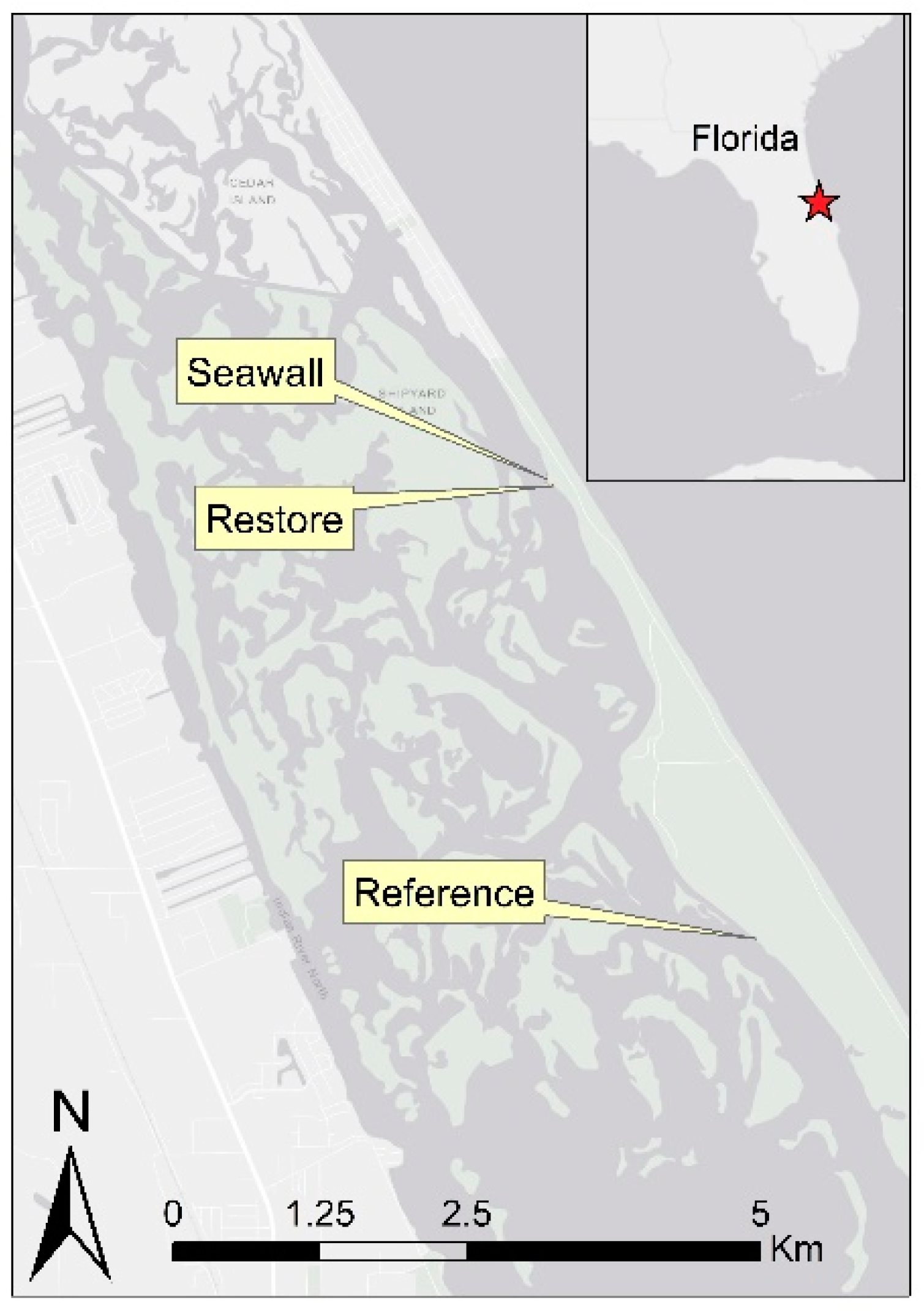
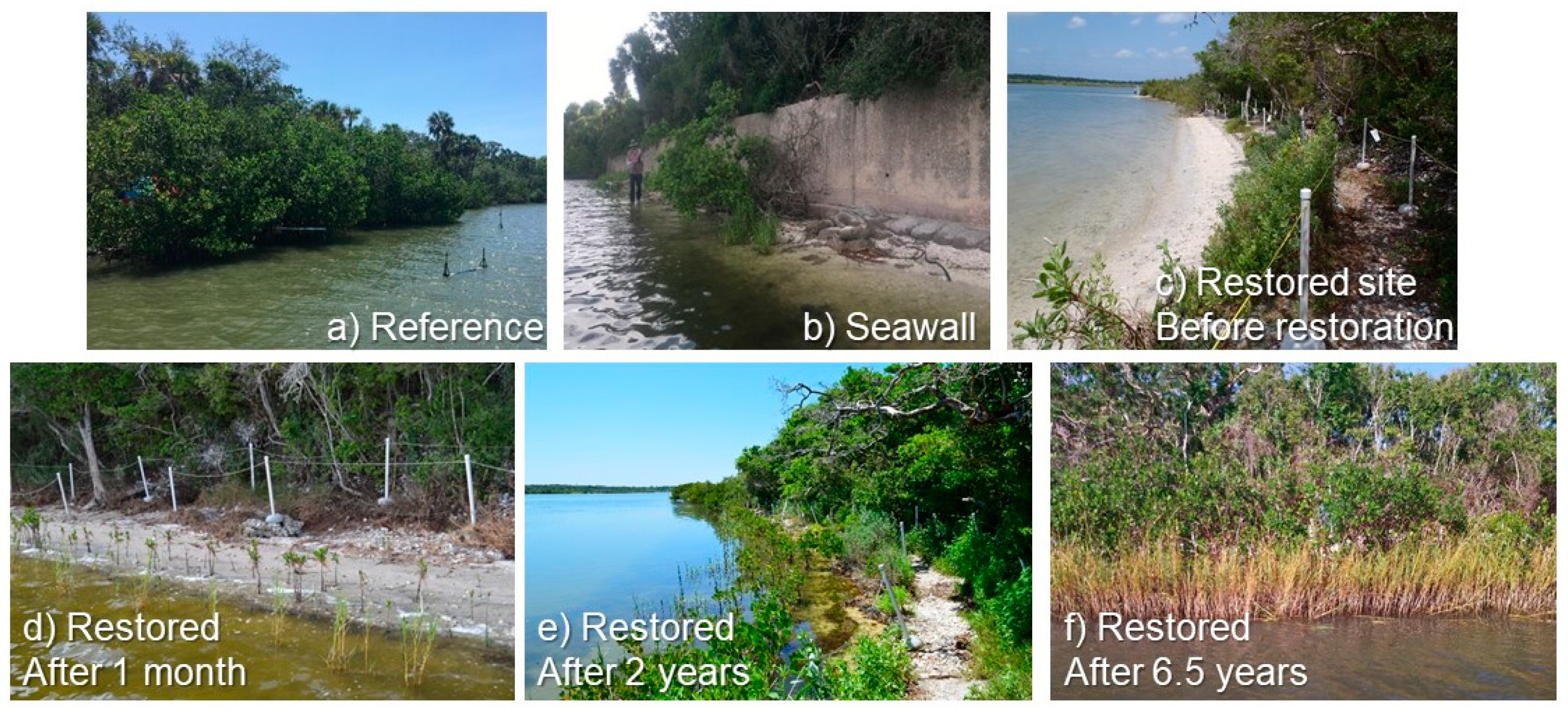
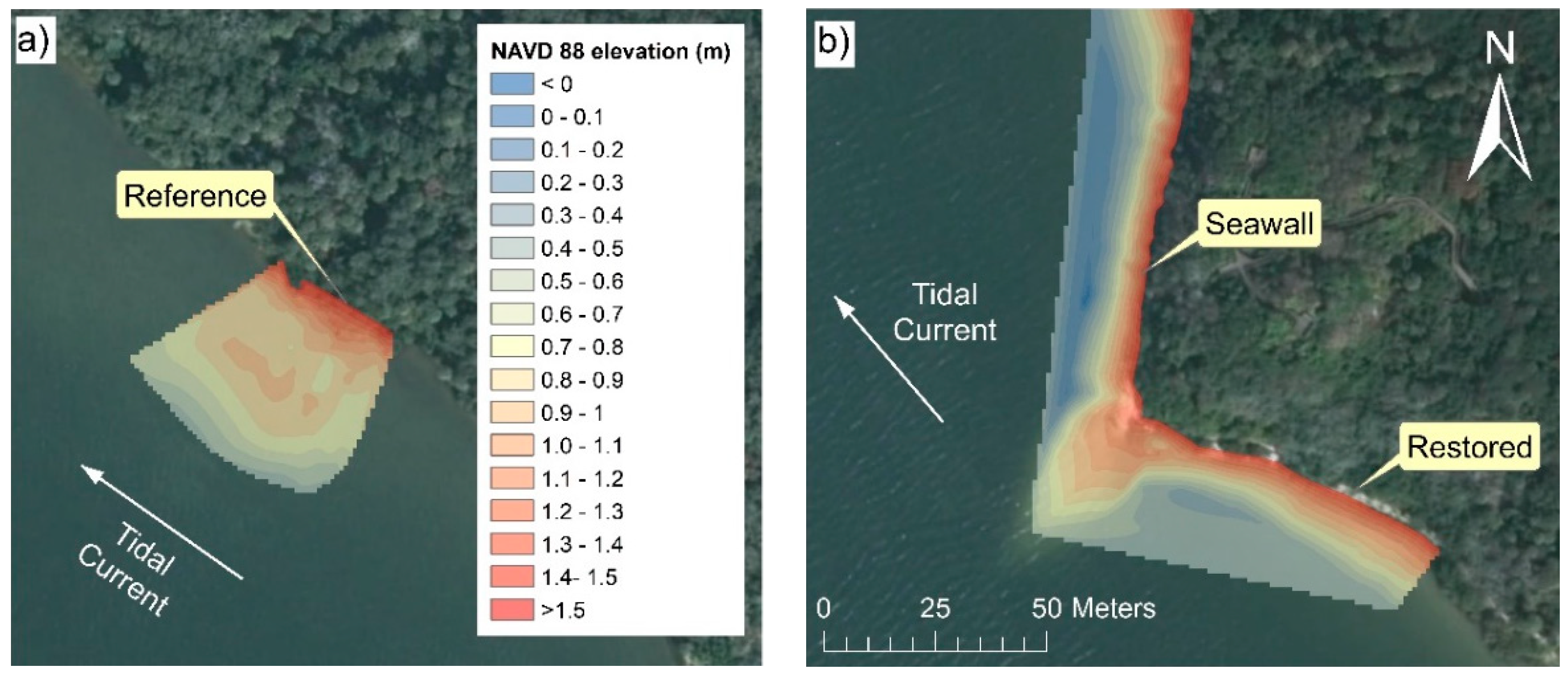
2.1. Study Site Description

Mosquito Lagoon is the northernmost of three estuarine lagoons comprising the extensive Indian River Lagoon system on Florida’s east (Atlantic) coast. As a bar-built estuary located between Florida’s mainland and barrier islands, Mosquito Lagoon is a wide, shallow (1–4 m water depth) water body containing numerous bars and vegetated islands within the main channel. Tidal exchange to the marine system occurs through an inlet in the northernmost portion of the lagoon, and a canal in the southern lagoon connects Mosquito Lagoon to the Indian River. Mosquito Lagoon is microtidal, with seasonal changes in water levels [32]. The climate is humid sub-tropical and the bulk of annual precipitation (mean 1250 mm yr⁻¹) is delivered as rain during the wet season from May through October. Salinity in Mosquito Lagoon ranges from 25 to 45 ppt [32]. The mean annual air temperature is 22 °C, and water temperatures range from 23 to 30 °C [33]. The barrier island comprising the east bank of the lagoon has a long history of human habitation dating to 500 B.C., and pre-historical shell middens [34] create an anthropogenically altered topography that stretches the length of the island.

Three 50-m to 100-m lengths of shoreline, consisting of one unrestored shoreline (Reference) and two restored sites (Restored—living shoreline restoration, Seawall—hybrid living shoreline stabilization) were selected for study from within a 4-km length of Mosquito Lagoon’s east bank in Canaveral National Seashore, Florida (Figure 1). The Reference site is a reference-condition shoreline with no evidence of active shoreline degradation. Vegetation in the intertidal zone of the Reference site is characterized by a stable, mature stand of mangrove forest (Rhizophora mangle, Avicennia germinans, Laguncularia racemosa) (Figure 2a). Prior to living shoreline restoration in 2011, the Restored site was actively degrading (Figure 2c). The restoration consisted of submerged oyster mats [35] and zoned plantings of emergent marsh grasses (Spartina alterniflora) and mangrove (R. mangle, A. germinans) (for details, see [36]). While early years following the restoration indicated moderate oyster recruitment to the mats (maximum 200 oysters/m²), a series of stochastic environmental events (e.g., brown tide algal bloom, drought, and historically low water levels) left recruited oysters vulnerable to predation and precipitated extensive mortality. At the time of data collection for this study, 6.5 years after restoration, few oysters inhabited the restoration site, and the mats had been either removed or buried by sediments and vegetation.

The Seawall site is a location of active net shoreline erosion. A retaining wall had been built near the shoreline in the 1950s, and erosion had progressed to the wall footing by 2012. Bags of cement had been placed at the footing in an attempt to stabilize sediments (Figure 2b). In 2013, stabilization of the eroding shoreline with a hybrid living shoreline was undertaken. The modified living shoreline consisted of 800 mesh bags filled with oyster shells (length:width:height = 100:30:30 cm) arranged in a low sill structure (one row deep, two rows wide), and plantings of smooth cordgrass (S. alterniflora). At the time of this study, four years after the hybrid living shoreline restoration, the structure was in place but buried by sediment, and only sparse vegetation remained on the Seawall shoreline in front of the retaining wall.

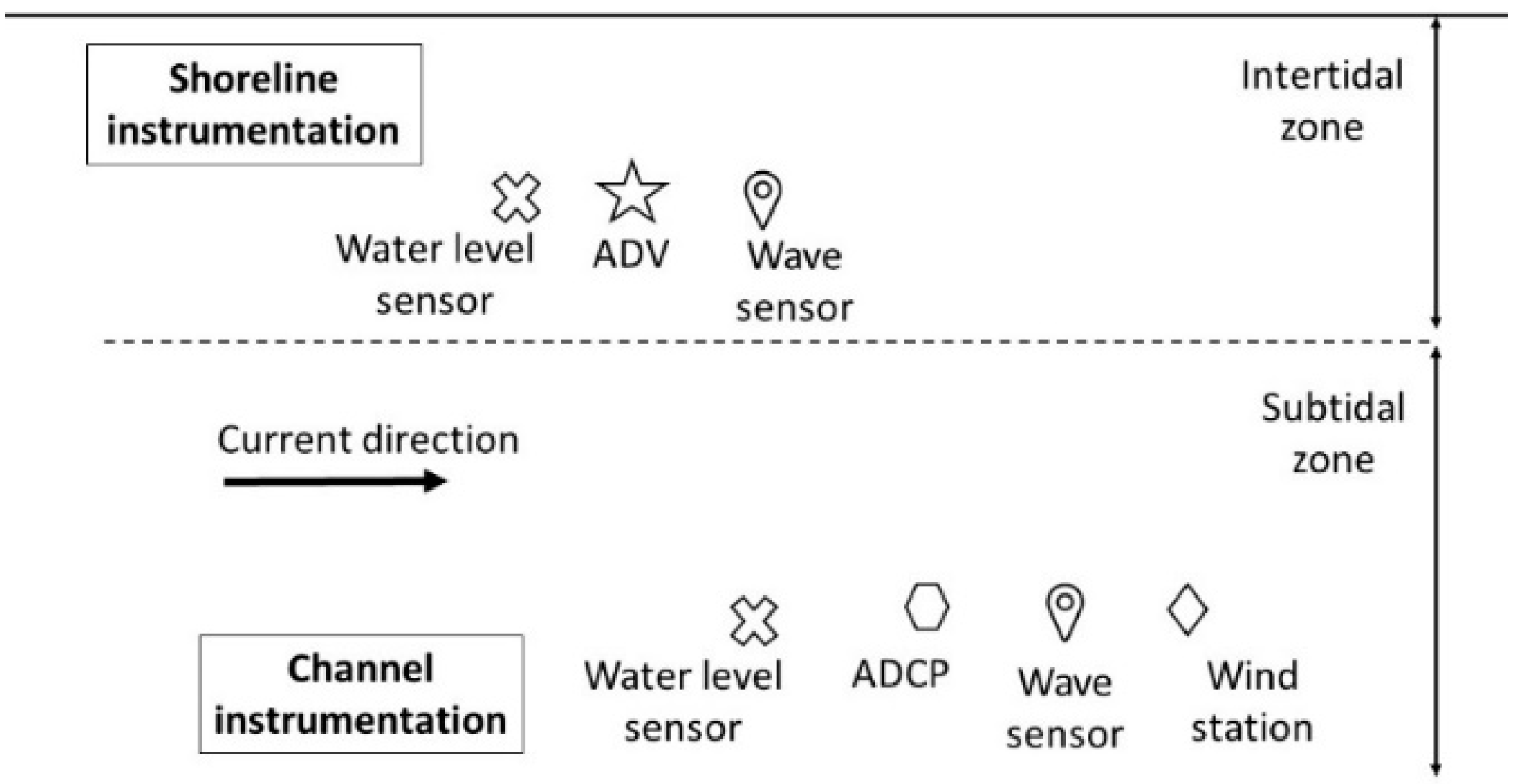
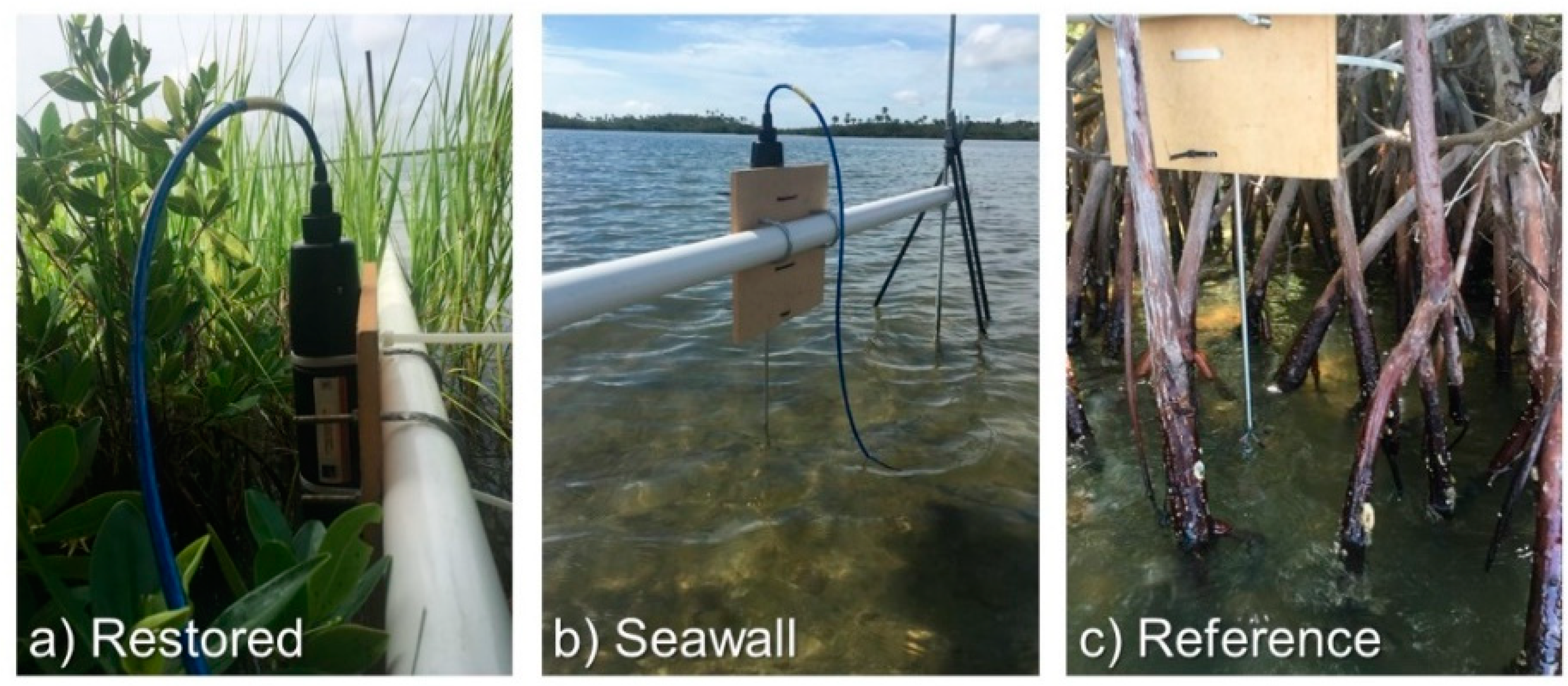
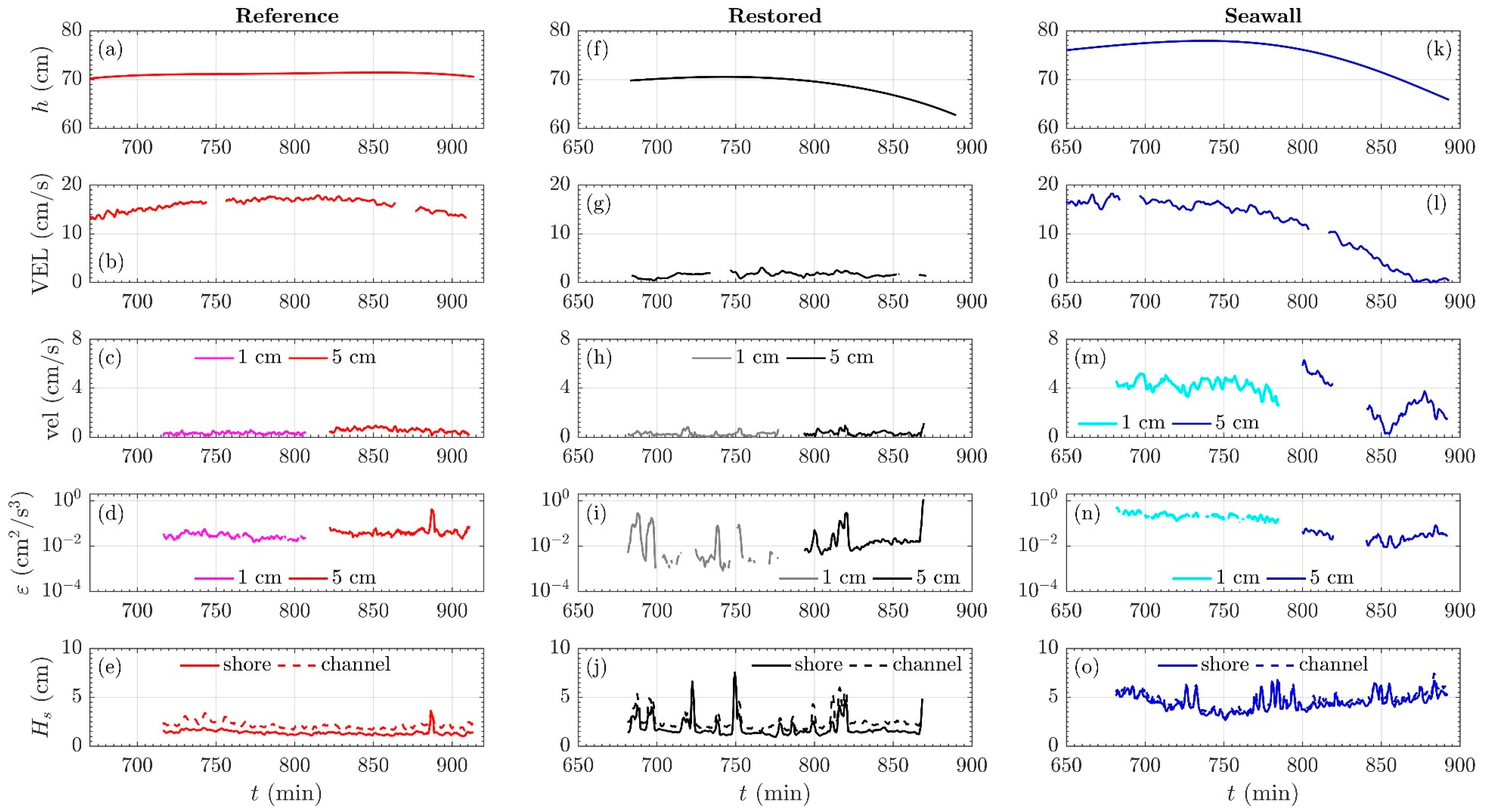
2.2. Field Data Collection

Field measurements were conducted on intertidal shorelines and in subtidal channels at seasonal low and high water levels, August and November 2017, respectively, 6.5 years after living shoreline restoration and four years after hybrid restoration. Between the two sampling periods, a sizable disturbance event, Hurricane Irma, occurred in September 2017. In each site, velocity profiles (15–20 mm vertical resolution) were sampled through the full water column at 2 Hz using a 2-MHz Acoustic Doppler Current Profiler (ADCP, Nortek), stationed down-looking in the channel, approximately 10 m offshore (Figure 3). The channel velocity sensor operated in burst sampling mode with either 6600 s of continuous measurements in a 7200-s period or 512 of continuous measurements over a 600-s period. All the instruments were aligned to a common coordinate system such that $u$, $v$, $w$ components of velocity respectively corresponded to streamwise (parallel to shore), cross-shore, and vertical directions. Velocity magnitude indicates flow strength, while directionality corresponds to the direction of the tidal pulse. Positive streamwise velocities corresponded to ebb tide (from south to north), while negative streamwise velocities were observed during rising tides (from north to south). Windspeed and direction in the channel were recorded 2 m above the water surface using a Davis Wind Speed and Direction Smart Sensor (Onset, S-WCF-M003) with a 60-s interval and 1-Hz sampling rate. Water depth was recorded at shoreline and channel monitoring positions at 60-s resolution (Onset, U20L-04). Water surface deformations in the channel and on shorelines were observed at 32 Hz using sonic sensors (Ocean Sensor Systems XB Pro).

Within each shoreline, 2–3 cm vertical velocity profiles (1-mm resolution) were sampled at 100 Hz, using a down-looking Vectrino Profiler (Nortek). Shoreline velocity data were collected in “high” and “low” probe positions, with respective sampling volumes located approximately within 3.2 to 6.6 cm and −0.5 to 2.1 cm above the bed, with minimal differences among the three sites. In order to observe the near-bed boundary layer, the low sampling volume intentionally intersected the bed. Although some data cells were discarded to avoid potential bed interference [37], this configuration positioned the highest accuracy portion of the profile (5 cm from the probe, [38]) at approximately 1.0 cm above the bed. At this height, local turbulence and flow resistance are affected both by the bed roughness and by characteristics of vegetation, if present. In the high probe position, the most accurate portion of the profile was collected around 5.0 cm from the bed. At this height, the bed effect should become less prominent, and the flow pattern will be more reflective of vegetation-induced drag.

All the sites were surveyed with a CHC X91 + Real Time Kinematic (RTK) GPS survey device referencing the North American Vertical Datum of 1988 (NAVD 88). Individual $xyz$ point data were surveyed by taking the mean of six corrected samples. Transects were surveyed at 2-m intervals from the shoreline to approximately 35 m into the channel. ASCII XYZ point data were converted to an elevation surface through raster interpolation using the natural neighbor algorithm. At the Restored and Reference sites, shoreline velocity profiles were collected within vegetation (Figure 4). Vegetation within a 0.25-m² quadrat in the immediate vicinity of the probe location was characterized for stem and prop root density ($n$), species, and diameter ($d$) at 10 to 20 cm above the bed. The density of roots and stems were combined to represent the total number of individual vegetation elements in each quadrat and are referred to as “elements” in the results below. Five additional 0.25-m² quadrats were randomly selected from each shoreline, and the vegetation within was characterized similarly. Two random transects were selected in each site, beginning at the most seaward extent of vegetation and continuing until wetland vegetation was no longer observed. Species within a diameter of 10–20 cm above the bed, and cohort (approximate age) were recorded for every mangrove seedling within a 1-m wide swath along transects.

Five sediment cores (approximately 200–300 g each) were collected to a depth of 20 cm from the shorelines and channels of each site, close to the locations of hydrodynamic data collection. Both sediments and water were retained within each core sample. Individual cores were dried in the lab at 110 °C for at least 24 h. Dry sediments were gently ground, sieved at 2 mm, and 20 g samples of the <2 mm size class were processed for loss on ignition at 550 °C for 16 h. Then, cores were pooled by site for an analysis of grain size distribution using dry and wet sieving.

2.3. Analysis of Hydrodynamic Data

2.3.1. Post-Processing and Quality Control

On the shorelines, precise probe distances from the bed were determined by the velocity profile and no-slip condition at the bed for the low position, and with the aid of the center beam amplitude for the high position. Center beam amplitude profiles (sampling rate 2 Hz) starting 2 cm from the probe until well below the bed were analyzed. The amplitude increased considerably at the bed due to the strong return signal from the solid boundary. The bed position was selected to coincide with the minimum amplitude gradient across the recorded profile [39,40]. The ambient environment of the lagoon provided a particle-rich environment for the proper detection of Doppler shift from both velocity sensors. As a result, the signal-to-noise ratio (SNR) and correlation for most of the measurements exceeded the thresholds suggested by Nortek for obtaining reliable measurements. Most shoreline measurements had SNR >30 dB and correlation >90%. Raw data with SNR <20 dB and/or correlation <80% (less than 2% of data) were removed from the time-series and gaps were interpolated linearly. Despite the high statistics in the measurements, some outliers in the velocity time-series may still exist [41]. The time-series was despiked according to the phase-space thresholding method suggested by Goring and Nikora [42] and modified by Wahl [43]. In the channel, most of the cells exhibited very high correlation (>90%), especially in the upper flow region. Measurements with correlation <70% were discarded. Such low correlation measurements occurred relatively close to the bed, which was presumably due to strong bed acoustic interference. Wakes generated by passing boats are not considered in this analysis. Wave data influenced by boat wakes were manually removed from the data time-series. No sediment transport or bed alterations were observed during the measurements.

To calculate channel-to-shoreline hydrodynamic gradients, the instantaneous velocity time-series were decomposed into segments of 120 s, across which flow characteristics were calculated. A moving average was applied, based on 30-s successive shifts of each 120-s segment along the flow velocity time-series, across which the flow is considered to be quasi-steady. Synchronous shoreline and channel velocity time-series were paired; the final datasets for each site consisted of 71 to 158 paired segments for each site and position.

2.3.2. Turbulent Kinetic Energy Dissipation

The presence of irregular waves precluded the direct calculation of turbulence intensity, as the sinusoidal pattern of wave orbital velocities affected the variance of the velocity time-series, which is needed to estimate turbulence intensity. Assessment of turbulence at shorelines was based on the dissipation rate of turbulent kinetic energy (TKE), $\epsilon$, as calculated using the structure function method [44] (Appendix A). This methodology utilizes Kolmogorov’s hypotheses for turbulence cascade and links TKE dissipation to the covariance of the velocity difference between two points [45] along the vertical velocity profile. Since wave oscillations decorrelate over larger scales [46,47], comparing velocities over such short distances leads to the effective filtering of wave-induced variance. As a result, velocity differences between profile points are attributed to turbulent eddies. Herein, a second-order structure function (Equation (1)), $D\left(z,r\right)$, was formed for the estimation of TKE dissipation rate at height $z$ above the bed, with vertical velocity fluctuations $w^{\prime }$ separated by distance $r$. By applying a centered difference technique, this takes the form:

$$D\left(z,r\right)=\overline{{\left[w^{\prime }\left(z-r/2\right)-w^{\prime }\left(z+r/2\right)\right]}^2}$$

(1)

where $w^{\prime }=w-\overline{w}$, with the overbar denoting time averaging over the 120 s of the moving average. Based on Taylor’s cascade theory, the structure function within the inertial subrange is also equal to [44,45]:

$$D\left(z,r\right)=C_v^2\epsilon {\left(z\right)}^{2/3}{r}^{2/3}$$

(2)

where $C_v^2$ is a constant equal to two [45]. For the calculation of dissipation $\epsilon$, linear regression was applied to Equation (3) between $D\left(z,r\right)$ and $r^{2/3}$, in order to derive an equation of the form:

$$D\left(z,r\right)=A{r}^{2/3}+N$$

(3)

where $A=C_v^2{\epsilon }^{2/3}$ and $N$ is error attributed to Doppler noise, which is independent of $r$ [44]. The mean dissipation rate was calculated for each 120 s of the moving average at each site and position, and was normalized by the corresponding root-mean-squared (rms) velocity, $u_{rms}$, to allow for comparison across sites and days. The rms velocity accounts for both current and wave variation [48] and is given by Equation (4):

$$u_{rms}=\sqrt{\overline{u^2}}$$

(4)

Data were evaluated to confirm assumptions of normal distribution and heterogeneity of variances. Current and wave attenuation and turbulent dissipation rates were compared using one-way analysis of variance (ANOVA) followed by Tukey post hoc pairwise comparisons to identify statistical significance ($\alpha =0.05$) between shoreline types (Restored, Seawall, Reference).

3. Results

3.1. Vegetation Characteristics and Shoreline Morphologies

Shoreline morphologies and characteristics of shoreline vegetation varied among sites. The mean width of the shoreline, as defined from the water’s edge at the mean low water level to the landward extent of hydrophytic vegetation, was over 25 m in the Reference site, less than 4 m in the Restored site, and below 2 m at the Seawall. Shoreline slopes in the Restored and Reference sites were similar (0.050 ± 0.001 and 0.056 ± 0.001, respectively) and considerably lower than slope of the Seawall shoreline (0.130 ± 0.005) (

Table 1. Intertidal and nearshore subtidal slope, characteristics of vegetation across random plots and in the immediate vicinity of shoreline flow observation (probe), and mangrove seedlings per transect meter in the Restored, Seawall, and Reference sites. Site mean and standard error or coefficient of variation (CV) are reported.

Site	Slope (m/m) Mean ± SE			Stem Density (n) (Elements/m2)		Frontal Area (α) (m2/m3)		Solid Volume Fraction (ϕ) (m3/m3)		Mangrove Seedlings Mean ± SE
	Intertidal Shoreline	Subtidal Nearshore	Overall	mean, CV	Probe	Mean, CV	PROBE	Mean, CV	Probe	Number per Transect m	Diameter (mm)	Cohort Age (years)
Restored	0.050 ± 0.001	0.051 ± 0.001	0.050 ± 0.001	97, 0.79	252	0.94, 0.59	1.62	0.012, 1.11	0.009	0.0 ± 0.0	0.0 ± 0.0	-
Seawall	0.130 ± 0.005	0.061 ± 0.001	0.110 ± 0.003	24, 1.64	0	0.20, 1.55	0.00	0.002, 1.59	0.000	0.0 ± 0.0	0.0 ± 0.0	-
Reference	0.056 ± 0.001	0.008 ± 0.001	0.027 ± 0.001	83, 0.39	116	2.49, 0.56	3.12	0.068, 0.74	0.070	4.0 ± 0.8	13.0 ± 0.5	1

, Figure 5). Vegetation at the Reference site consisted of a mature stand of mangrove forest. Forest fringing the channel was inundated at all seasonal and tidal water levels, and emergent vegetation consisted primarily of R. mangle prop roots with a mean density of 83 elements/m², mean diameter of 28 mm, and solid volume fraction of 0.068. Many mangrove seedlings were observed in 1-m wide transects of the Reference site (4 ± 0.8 per transect meter, Table 1), consisting of R. mangle, A. germinans, and L. racemosa. The majority of the Seawall site was unvegetated. Remaining vegetation consisted of one sparse patch of S. alterniflora. In the Restored shoreline, restoration converted a shoreline of bare sediment (Figure 2c) to a fully vegetated shoreline with up to 85% vegetation coverage (Figure 2f and Figure 6). Six years after restoration, vegetation in the Restored shoreline consisted of S. alterniflora, R. mangle, and A. germinans that had been planted during the restoration, or in the case of S. alterniflora, had propagated vegetatively from plantings. The site’s heterogeneous emergent vegetation consisted of both S. alterniflora stems/leaves and young R. mangle stems/prop roots and comprised a greater number of smaller elements (mean density of 97 elements/m² and diameter of 10 mm) as compared to the fewer, large elements in the mature Reference site. The frontal element area per unit volume ($\alpha$) and solid volume fraction ($\varphi$) were both greater in the Reference site (Table 1). No mangrove seedlings were observed in transects of the Seawall or Restored site.

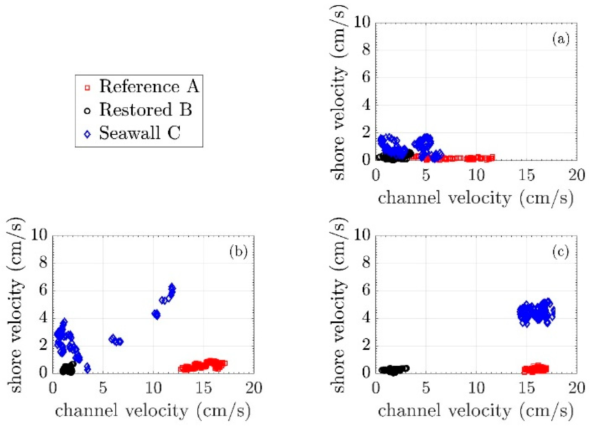
3.2. Mean Current Attenuation from Channel to Shoreline

Depth-integrated channel velocities varied between sites and days, ranging from near zero during periods of tidal stagnation up to nearly 20 cm/s during peak tidal exchange (Figure 7). In all the shorelines and channels, streamwise velocities dominated the flow field. The shoreline velocities (1.0 and 5.0 cm above the bed) of all the sites were generally lower than the depth-integrated channel velocities, reflecting typical flow profile behavior (Figure 8). However, current attenuation rates from channel to shore differed across sites (

Table 2. Mean ± SD significant wave heights and current velocities observed in shorelines and channels at the Restored, Seawall, and Reference sites.

	Waves			Current
	Nov 2017 Significant Wave Height (cm)			Aug 2017 1.0 cm Above Bed (cm/s)			Nov 2017 1.0 cm Above Bed (cm/s)			Nov 2017 5.0 cm Above Bed (cm/s)
	Channel	Shoreline	Percent Change	Channel	Shoreline	Percent Change	Channel	Shoreline	Percent Change	Channel	Shoreline	Percent Change
Restored	2.4 ± 0.2	1.4 ± 0.1	36 ± 8	1.9 ± 0.8	0.3 ± 0.1	83.8 ± 12.0	1.6 ± 0.5	0.2 ± 0.1	86.9 ± 8.1	1.5 ± 0.3	0.3 ± 0.1	80.1 ± 9.3
Seawall	4.8 ± 0.8	4.5 ± 0.8	7 ± 6	3.9 ± 1.5 +	0.9 ± 0.4 +	74.4 ± 16.1 +	16.0 ± 0.9	4.4 ± 0.4	72.3 ± 2.5	5.8 ± 4.1 +	2.9 ± 1.8 +	36.4 ± 39.3 +
Reference	2.2 ± 0.4	1.4 ± 0.3	35 ± 6	7.6 ± 2.3	0.2 ± 0.1	97.6 ± 1.8	16.1 ± 0.5	0.3 ± 0.1	98.2 ± 0.5	15.2 ± 1.2	0.6 ± 0.2	96.2 ± 1.0

⁺ when channel velocity exceeds 1.5 cm/s.

,

Table 3. Results of one-way ANOVA for wave and current attenuation rates from channel to shore, and normalized turbulent kinetic energy (TKE) dissipation at the Restored, Seawall, and Reference sites.

	Mean Square	df	F-Stat	p-Value
Wave Attenuation Rate	9.20 *	2	2694.57	<0.001
Current Attenuation 1.0 cm Above Bed	3.32 *	2	475.94	<0.001
Current Attenuation 5.0 cm Above Bed	6.23 *	2	216.89	<0.001
Normalized TKE Dissipation Rate	0.68 *	2	1660.89	<0.001

* significant at the α = 0.05 level.

and

Table 4. Pairwise comparisons of wave and current attenuation rates from channel to shore, and normalized TKE dissipation at the Restored, Seawall, and Reference sites.

Comparison	Wave Attenuation Rate		Current Attenuation Rate				Normalized TKE Dissipation Rate
			1.0 cm Above Bed		5.0 cm Above Bed		5.0 cm Above Bed
	Mean ± SE Difference (%)	p-Value	Mean ± SE Difference (%)	p-Value	Mean ± SE Difference (%)	p-Value	Mean ± SE Difference (m−1)	p-Value
Restored-Seawall	29.0 ± 0.7 *	<0.001	12.3 ± 0.9 *	<0.001	43.7 ± 3.1 *	<0.001	0.06 ± 0.003 *	<0.001
Restored-Reference	0.5 ± 0.7	0.780	−12.5 ± 0.9 *	<0.001	−16.1 ± 2.3 *	<0.001	−0.08 ± 0.010 *	<0.001
Reference-Seawall	28.6 ± 0.4 *	<0.001	24.8 ± 0.8 *	<0.001	59.8 ± 2.9 *	<0.001	0.14 ± 0.002 *	<0.001

* significant at the α = 0.05 level.

). Vegetated shorelines (Restored and Reference) attenuated currents at greater rates than the unvegetated Seawall site (p < 0.001 at both 1 cm and 5 cm above the bed). Additionally, currents were more strongly attenuated by mature mangrove vegetation in the Reference shoreline as compared to vegetation at the Restored site (p < 0.001 at both 1 cm and 5 cm above the bed). In vegetated sites, flows consistently decelerated from the channel to the shoreline (Figure 8). The mean horizontal near-bed (1.0 cm above bed) shoreline velocities in the Restored and Reference sites were respectively 84–87% and 98% lower than channel velocities. By comparison, near-bed shoreline velocities at the Seawall site were 72–74% lower than the channel velocities. Shoreline flows 5.0 cm above the bed for the most part exceeded the near-bed velocities due to the reduced bottom drag being higher within the boundary layer, but the flows were lower than the channel speeds. Similar to the near-bed results, the velocity reduction from channel to shore at the Restored and Reference sites was high (80% and 96%, respectively) relative to the Seawall (36% reduction when channel velocities exceeded 1.5 cm/s). The differences in current attenuation between sites were more pronounced 5 cm above the bed (Table 3), reflecting a lowered influence of bed interaction and stronger interaction with vegetation higher in the flow profile.

When channel currents fell below 1.5 cm s⁻¹, behavior at the Seawall shoreline became unpredictable, and the shoreline velocities often greatly exceeded the channel depth-integrated flows. For instance, mean shoreline velocities up to 3.0 cm/s were observed when channel velocities were below 0.6 cm/s. Such erratic behavior reflects the pronounced hydrodynamic influence of waves in the unvegetated site during times of stagnant current. By comparison, within vegetation, the mean shoreline flows were consistently suppressed to below 0.90 cm/s, even when the channel flows were of relatively high magnitude (e.g., exceeding 17 cm/s in the channel near the Reference site). When similarly high channel forcings were observed in the Seawall site, the mean shoreline flows were far greater: consistently above 4 cm/s.

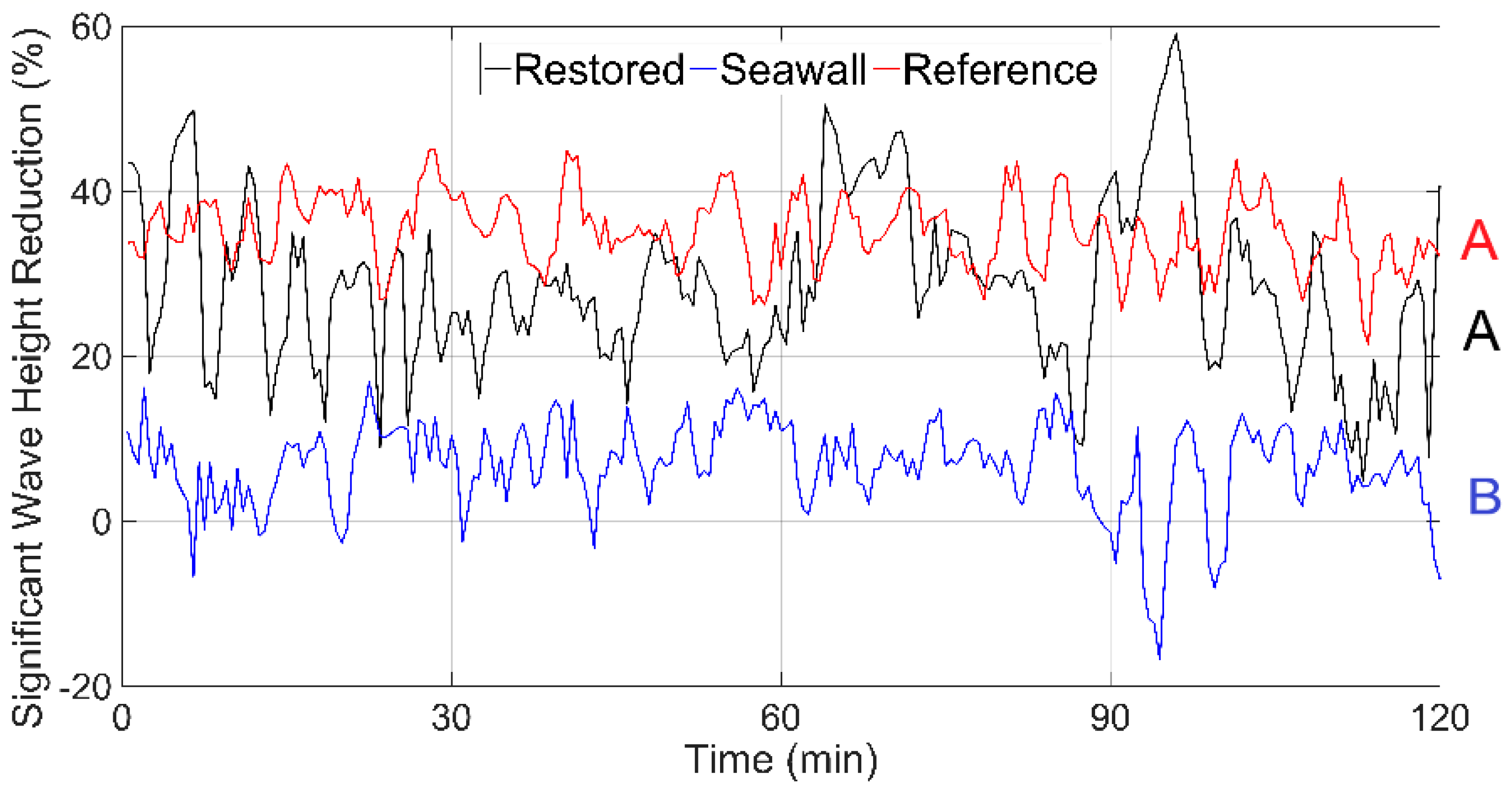
3.3. Wave Attenuation from Channel to Shoreline

Significant wave heights ($H_s$, defined as the mean of the top 1/3 wave heights, here computed across each moving average period) observed in the channels and on the shorelines at all the sites were low (<8 cm significant wave heights) and generally corresponded with prevailing wind conditions. The mean significant wave heights observed at the Seawall site (4.8 ± 0.8 cm in channel, 4.5 ± 0.8 cm on shoreline) were larger than those observed at the Reference site (2.2 ± 0.4 cm in channel, 1.4 ± 0.3 cm on shoreline) and the Restored (2.4 ± 0.2 cm in channel, 1.4 ± 0.1 cm on shoreline) site. Wave heights typically decreased from the channel to onshore (Figure 9), with stronger and more consistent attenuation observed within the vegetated sites (p < 0.001, Table 3 and Table 4). Significant wave heights decreased from the channel to shoreline by a mean of 36 ± 8% and 35 ± 6% within the Restored and Reference sites respectively, while mean wave attenuation was 7 ± 6% at the Seawall site. Wave attenuation was similar in the Reference and Restored shorelines (p = 0.780). Comparing periods of similar channel wave heights across sites further confirmed that the vegetated sites attenuated waves more efficiently than the unvegetated site. When the offshore wave heights were 3–4 cm, attenuation was greatest at the Reference site (32 ± 17% reduction), followed by the Restored site (22 ± 9% reduction). By comparison, attenuation at the Seawall site was low (7 ± 4% reduction). Offshore wind waves exceeding 4 cm were not observed at the Reference or Restore sites; however, wakes from passing boats were observed to exceed 7 cm in the channel off the Restored site. When offshore wave heights ranged from 4 to 8 cm, attenuation at the Restored site (23 ± 21% reduction) was greater than at the Seawall site (7 ± 6% reduction).

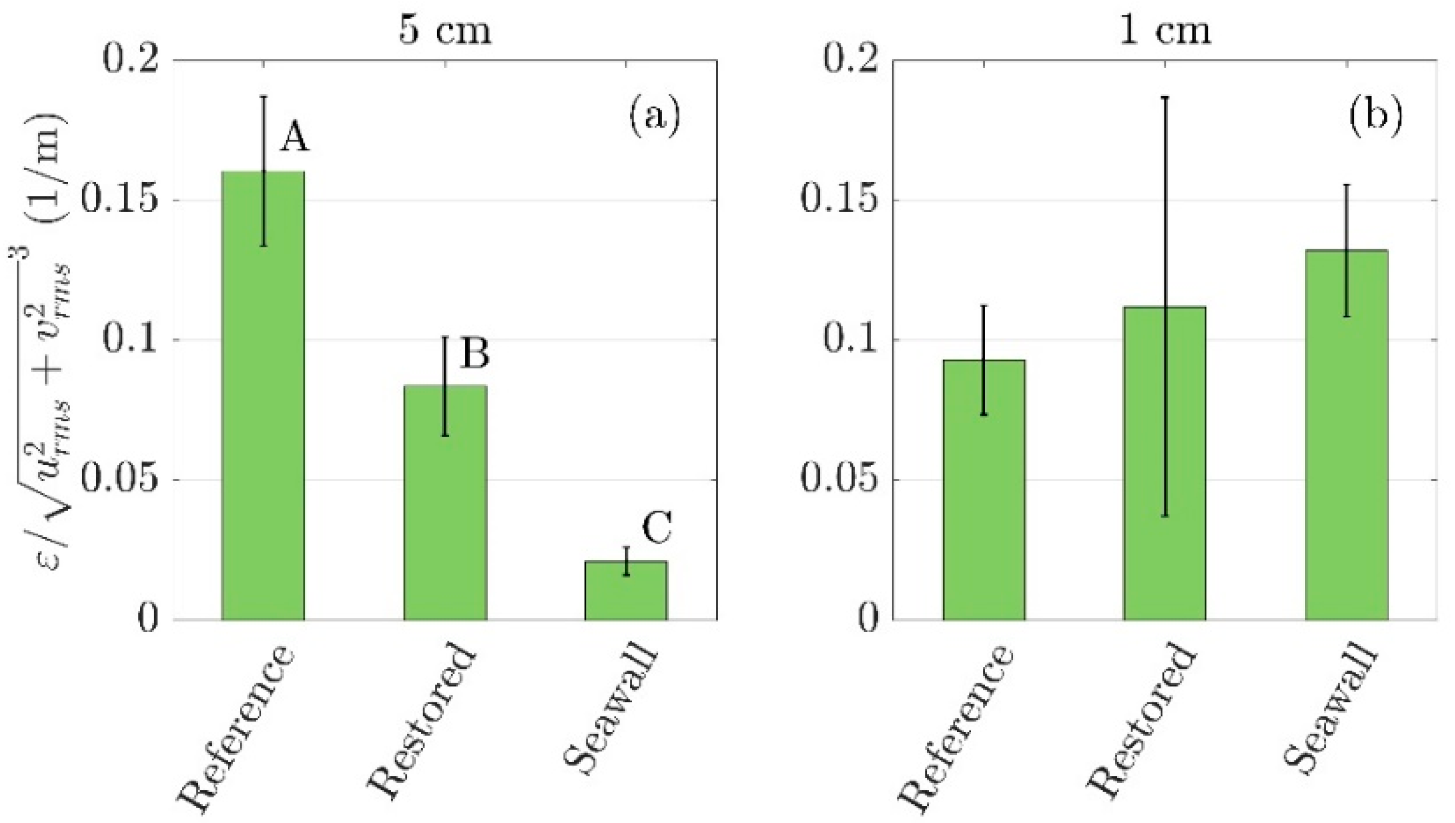
3.4. Comparison of Turbulent Kinetic Energy Dissipation across Sites

The linear regression that was applied in Equation (3) had a very good fit with the measurements 5.0 cm above the bed, with $R^2>0.90$. However, data fit closer to the bed was variable, and a cutoff threshold was established at $R^2=0.85$, below which measurements were discarded. The number of points utilized for the linear regression was respectively eight, 11, and 10 for the high position in the Reference, Restored, and Seawall sites, while it was consistently five for measurements at the low position for all the sites. For the low position, no velocities recorded within 4 mm of the bed were utilized, due to potential bed interference in the signal in near-bed measurements [37]. At 5 cm above the bed, the normalized TKE dissipation rate was highest at the Reference site (0.16 ± 0.03 m⁻¹), followed by the Restored (0.08 ± 0.02 m⁻¹) site, and the Seawall (0.02 ± 0.01 m⁻¹) site (p < 0.001, Table 3, Figure 10). However, 1 cm above the bed, the three sites exhibit similar normalized dissipation rates (Reference: 0.09 ± 0.02 m⁻¹, Restored: 0.11 ± 0.07 m⁻¹, and Seawall: 0.12 ± 0.03 m⁻¹).

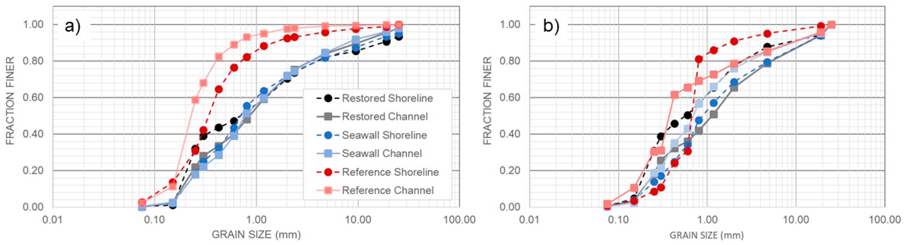
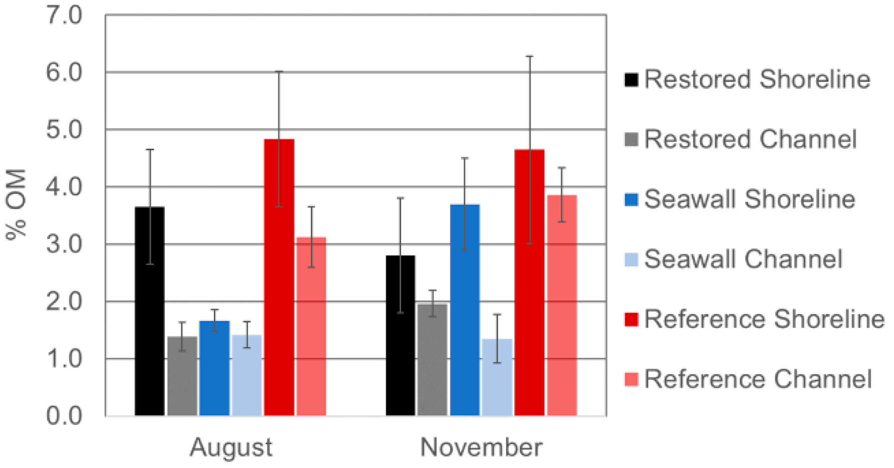
3.5. Comparison of Sediments across Sites

The bulk of sediments at all the sites consisted of coarse to fine sand. Larger particles were shell fragments, comprising up to 30% of particles by mass in the Restored and Seawall sites. Only small fractions of silt/clay were observed; these generally comprised less than 3% of the sample mass. Before Hurricane Irma, the texture of sediments in the Restored and Seawall sites were similar, and notably coarser than the Reference site sediments (Figure 11a). Surprisingly, the finest sediments were found in the channel just off the Reference shoreline, while sediments within the mature mangrove forest were slightly coarser. Changes to sediment distributions were detected in all the sites after Hurricane Irma (Figure 11b). Immediately after the hurricane, shoreline sediments at the Reference site coarsened (Figure 11b), with $d_{16}$ and $d_{50}$ increasing from 0.15 to 0.40 mm and from 0.18 to 0.60 mm, respectively. Within the mangrove vegetation $d_{84}$ remained relatively stable, but increased in the channel from 1.00 mm to 2.40 mm (Figure A1). The observed changes account for the deposition of medium to coarse sand within the Reference vegetation. A similar sediment deposition within vegetation also occurs at the Restored shoreline. Here, shoreline $d_{16}$ and $d_{50}$ remained relatively stable, but $d_{84}$ decreased notably from 6.60 to 2.20 mm due to coarse sand deposits. Meanwhile, the opposite trend in $d_{84}$ was noted in the Restored channel, coarsening after the hurricane from 4.75 to 6.30 mm, which was similar to changes observed in the Reference channel. Few changes were detected to shoreline particle distributions at the Seawall site.

Organic matter (OM) content tended to be higher in the shoreline rather than channel sediments. However, at the Seawall before the hurricane, the channel and shoreline OM contents were similarly low. Sediments of vegetated shorelines contained greater percentages of carbon (respectively 4.84 ± 1.32% and 3.65 ± 1.00% in the Reference and Restored shorelines) compared to the channel and unvegetated shoreline sediments (e.g., 1.67 ± 0.21% in the Seawall shoreline) (Figure A2). Mimicking particle size results, the channel sediments off the Reference shoreline, just outside of the mature mangrove vegetation, contained high percentages of OM (3.12 ± 0.59%), which were levels that were well above the shoreline sediments in the Seawall site. Immediately after the hurricane, effects of sediment reorganization were evident. Shoreline and channel OM content became more similar at the vegetated sites, likely reflecting the large transport and deposition of sand from the channel into the vegetated shorelines during the event. However, OM content increased substantially in the Seawall shoreline, up to 3.70 ± 0.89%. During sample collection, it was observed that copious quantities of seagrass wrack had been deposited in the Seawall shoreline after the hurricane [49], which likely accounts for the increased OM content found in the sediments.

4. Discussion

4.1. Differential Hydrodynamic Effects of Bare Sediment, Restored Vegetation, and Natural Vegetation

Near-bed shoreline velocities were consistently lower than depth-integrated channel velocities at all the sites and sampling periods, which is typical flow behavior at channel margins. Similarly, wave heights at shorelines were consistently smaller than those observed in the channels, which also was expected behavior for waves across differing water depths. However, flows were consistently more strongly attenuated in the vegetated sites (Table 2, Figure 8 and Figure 9), with the greatest attenuation rates observed in mature mangrove vegetation (Table 4). Notably, shoreline velocities within the mangrove prop roots of the Reference site remained extremely low, even when velocities in the channel become relatively strong. By comparison, at similar channel flows, velocities in the unvegetated Seawall shoreline often exceed velocities in the Reference shoreline by an order of magnitude. Comparable strong current speeds were not observed in the channel near the Restored shoreline. Therefore, while we can conclude that the planted vegetation attenuated the current at low speeds, the performance at greater currents speeds (such as those observed at the Reference site) cannot be verified. However, at larger wave heights, wave attenuation is high in planted vegetation compared to the unvegetated Seawall site.

The observed current and wave attenuation in vegetation underscores many past laboratory and field studies that reported similar conclusions regarding the effects of emergent vegetation on flows [22,50,51,52,53]. However, this is one of the first detailed comparisons of flow attenuation between reference state vegetation and restored vegetation based on field observations. The primary hydrodynamic interaction of flows within vegetation is related to an increase in flow resistance due to drag force against the vegetation, leading to slower mean flows within vegetation [54]. This effect can be clearly observed as a significantly greater current attenuation in vegetated versus unvegetated shorelines, both near-bed and higher within the flow profile at 5 cm above the bed (Table 2 and Table 4). Furthermore, the greater difference in current attenuation rate at sites at 5 cm above the bed as compared to near-bed illustrates the different mechanisms of flow resistance in vegetated and non-vegetated shorelines. Near the bed, attenuation in the vegetated and unvegetated sites was more similar, as the bed boundary strongly influenced all the sites. Higher in the flow profile, the interaction with vegetation became a more significant source of flow resistance, and much stronger differences in flow attenuation were observed between the vegetated and unvegetated sites.

Prior study comparing flow attenuation through emergent marsh grasses and mangroves [55] report conclusions similar to the present study: mangrove vegetation is more effective in attenuating current than emergent marsh grasses, although herein much greater levels of flow attenuation were observed for similar bare channel current speeds. Observations reported from prior study [55] were additionally only true when the mangrove canopy was also submerged, which did not occur in this study. The presented data suggest that differences in vegetation morphologies, densities, or configuration alone are sufficient to produce the observed stronger flow attenuation through mature mangrove vegetation. Flow and wave attenuation rates at all the sites were similar across the nominal range of observed water level variations (0.2 m) within the microtidal environment. Past research has observed strong nonlinearities in flow attenuation when water level variation exceeded biological thresholds [55,56]. The results reported herein demonstrate the resilience of emergent vegetation to attenuate flows across small variations in water levels. While the wave attenuation observed at the Seawall site was low relative to the vegetated sites, attenuation rates were also consistent across the observed water levels. This observation suggests that wave attenuation at the Seawall was driven by a consistent nearshore slope and not affected by the low modular structure comprised of oyster shell bags deployed during hybrid restoration. No topographic traces of the oyster shell bag structure remained (Figure 5) after burial by a deep and uniform layer of sediments.

Turbulent Kinetic Energy Dissipation Rate

While mean flow magnitudes in vegetation may be reduced, eddies shed from the interaction of flows with vegetation components (stems, leaves, prop roots) increased the intensity of turbulent fluctuations [25,57]. Important consequences to sediment transport in vegetation derive from the combination of competing effects to mean and turbulent flows [25]. The observed difference in turbulence dissipation from the near-bed (1.0 cm from bed) as opposed to 5.0 cm above the bed allows for understanding the partitioning between bed and stem-generated turbulence (Figure 10). Observations near the bed include turbulence generated at the flow–bed boundary, and in vegetated sites, also by the flow-stem interaction. Higher within the water column, the effect of the bed boundary was smaller, and the relative contribution of the stem-generated turbulence may be inferred. We observe that the magnitudes of the turbulence dissipation rate (normalized to local flow condition) and the partitioning of turbulent dissipation between the bed and stems varied between sites. Five centimeters above the bed, normalized turbulent dissipation was significantly greater in vegetated shorelines. The difference in dissipation rates observed at the vegetated and unvegetated shorelines may reflect systematic differences in advected turbulence within obstructed versus unobstructed flows. For example, within rough canopies, the production and dissipation of turbulence may be imbalanced due to an advection of eddies shed from upstream obstructions [58]. It is likely that the greater dissipation rates observed in the vegetated sites reflect not only the local production of turbulence, but also include a greater input of advected turbulence shed from the stems immediately upstream. The turbulence dissipation rate 1.0 cm above the bed was relatively balanced for all three sites, which highlights the dominant effect of bed-generated turbulence in near-bed flow regions.

Interestingly, turbulent dissipation was significantly greater in the Reference shoreline than the Restored shoreline, which was similar to how the current attenuation was also significantly greater. The differences in current attenuation rates and normalized dissipation rates observed in the two vegetated sites likely reflect variable drag, turbulence production, and advection from the differing vegetation morphologies. Although both sites are vegetated, the vegetation characteristics are markedly different (Table 1). The mature R. mangle prop roots that dominate vegetation in the Reference shoreline create an array of relatively sparse, larger elements that are approximately cylindrical above typical water levels, but have varied rough morphology (through the recruitment of barnacles and oysters) in subtidal portions of stems (Figure 4c). In addition, TKE in the wake of the prop roots is likely affected by the variation in the projected frontal area with height, as the prop roots project a bell-shaped rather than rectangular frontal area (Figure 4c) [59]. Thus, the solid volume fractions represented by assuming that mangrove roots are regular cylinders with diameters similar to above the typical water level are likely to be underestimations. In addition, irregularities in the vertical variation of the frontal area of an obstacle could lead to vertical mixing in the wake, which enhances the turbulence generated from the stems [60]. At the Restored site, the young mangrove roots and S. alterniflora grass stems and leaves created arrays with more and thinner elements, compared to the Reference site, with varied cross-sectional morphology (Figure 4a). These array and morphological differences may partially explain the differences in current attenuation and dissipation rates observed in the Reference and Restored sites.

Analyzing the turbulence from field data influenced by both waves and current can be challenging, as it can be difficult to isolate turbulent fluctuations from periodic oscillations due to non-regular waves. The methodology applied herein to estimate the TKE dissipation rate was originally developed for deep flows in the marine environment [44]. However, more recently, it has been utilized in surf and swash zones [61,62], salt marsh vegetation [63], and flows through mangroves [46,47,64]. The actual turbulence dissipation rates observed in this study are much lower than the rates reported by Norris et al. [47,64], who observed turbulence dissipation rates up to $6.5·{10}^{-4}$ m²/s³ in pneumatophores of black mangroves. However, both current velocity and wave heights were greater in the pneumatophores. Additionally, the structure of black and red mangrove vegetation is different. Pneumatophores are rigid stems that protrude into the flow and usually become fully submerged during high tide. The vegetation studied herein remained fully emergent across the range of flows observed. Almost all the normalized dissipation rates reported in [64] are more than an order of magnitude lower than the normalized TKE dissipation rates reported in this study, although different normalization factors were applied. Norris et al. [64] normalized dissipation by simultaneous current and orbital velocity measurements in the free-stream above the pneumatophore canopy rather than by root-mean-square velocities. Thus, it is unclear whether differences in normalized dissipation can actually be attributed to the greater turbulence observed within red mangroves and S. alterniflora or whether the normalization differences between the two studies preclude their direct comparison.

4.2. Mangrove Recruitment into Restored Shorelines

Long-term restoration success ultimately hinges upon the natural recruitment of desired species into restored areas. The retention and establishment of the first mangrove seedlings can indicate that a restored site has achieved a critical tipping point in habitat suitability. For example, Kamali and Hashim [65] observed the natural recruitment of Avicennia marina propagules within eight months following the installation of a wave break. In this study, 6.5 years after restoration, the growth of wetland vegetation planted at the Restored shoreline was substantial and had demonstrably altered the shoreline habitat with respect to cover and hydrodynamics. Past research indicated that propagules were supplied by dispersal from nearby mature mangrove stands and within-site reproduction, and that supply was not limited at the Restored shoreline [15]. An increased cover of vegetation following restoration, particularly of S. alterniflora, was expected to support mangrove recruitment by “propagule trapping” to promote retention and establishment [17,66,67]. Yet, naturally recruited mangrove seedlings were not observed in the restored vegetation. By comparison, hundreds of recruited seedlings were counted during the same year in the Reference site, where a mean of four seedlings were observed along each 1-m wide band transect meter. The recruitment rates observed in the nearby reference areas may indicate levels of recruitment that can sustain a site long-term and support observations that propagule supply was not a limiting factor at the Restored shoreline.

A detailed analysis suggests that the hydrodynamic limitations to mangrove recruitment do not explain the lack of observed recruitment at the Restored site. Shoreline hydrodynamic forces were similar in magnitude to those observed at the Reference site, where mangrove recruitment was evident. Rather, other limiting factors can perhaps explain the observed recruitment rate differences. For instance, sediment and morphological characteristics differed in the Restored and Reference shorelines. Sediments in the mature mangrove forest were finer in texture and contained more organic matter than those at the Restored shoreline, which more closely resembled sediments from the bare Seawall shoreline. The nearshore slope leading into the mangrove forest at the Reference site was very low; nearshore channel sediments were fine, and contained high organic matter content. This may suggest that the influence of the mangrove vegetation extends well beyond the actual vegetated zone. As flows approaching the vegetation are attenuated, it is possible that suspended materials are deposited upstream, over time creating a long, shallow, low-gradient approach to the shoreline. Similar morphology and fine channel sediments were not observed at the Restored site. Although vegetation cover was high, shoreline slopes were similar to the Reference shoreline, and flows were well attenuated; 6.5 years after restoration, sediments and nearshore (subtidal) slopes in the Restored site still carried evidence of the site’s history. Prior to stabilization, severe erosion of the shoreline into the adjacent shell midden provided a consistent source of large shell fragments to the shoreline. The years of site degradation prior to restoration had a greater fraction of large particles, as smaller fractions were selectively winnowed from the shoreline. The nearshore slope had perhaps not yet had time to reflect the morphologic adjustments to sediment transport initiated by the addition of vegetation to the shoreline. Such lingering indicators of sediment and morphology serve to remind that restoration impact requires time. While some effects—such as vegetation growth and related changes to hydrodynamics—can be observed relatively quickly, their long-term influence to morphology may manifest over longer timescales. Thus, thresholds in habitat suitability for mangrove recruitment may take time to achieve, even when hydrodynamics suggest that a site should be functionally similar to a reference condition. Given the significant time investment that may be required to create a functional shoreline from a degraded state, intact shoreline ecotones must be recognized as the green infrastructure asset that they are, and be preserved at all cost.

4.3. Why Did Vegetation at the Restored Site Thrive While Hybrid Restoration at the Seawall Did Not?

Vegetation planted during restoration was able to readily establish and flourish in the Restored site, while planted vegetation was not able to persist in the Seawall site, which was stabilized using a hybrid living shoreline approach. The analysis presented herein suggests that the Restored site was successful because, from a hydrodynamic perspective, it was well-suited for the applied living shoreline restoration technique. Although the two sites are contiguous, the unique geographies of each create very different hydrodynamic environments (Figure 7), which influence the shoreline and nearshore morphology. The Seawall and Restored shorelines occupy opposite sides of a point that protrudes into the main channel; thus, their aspects differ relative to the predominant current direction (Figure 5). Furthermore, the Restored shoreline is located within a small embayment. The effect of geography to current exposure is evident. Channel currents observed at similar distances from the shoreline at the same portion of the tidal cycle on contiguous sampling days were consistently greater at the Seawall site than at the Restored site (Figure 8). In addition, the intertidal slope of the Restored shoreline was much lower than the shoreline slope in front of the Seawall, similar to the slope observed in the Reference shoreline. The observed incoming waves were larger in the Seawall channel (Figure 7). Even with similar wind exposure (all the sites had similar fetch), waves were consistently larger at the Seawall, potentially due to the greater channel slope.

The lower slope observed in the Restored shoreline, compared to the Seawall, may itself have been an effect of the planted vegetation; however, the restoration did not include manual site grading. Alterations to the Restored shoreline slope would have manifested after restoration due to changes in sediment deposition and scour patterns. However, the similar sediment grain-size distributions found at the Seawall and Restored sites (pre-Hurricane Irma) suggest that such changes may have been nominal, even 6.5 years after restoration. It is rather more likely that the slope of the Restored shoreline was low before restoration. The combination of lower-energy hydrodynamic conditions and lower topographic gradients from the shoreline to channel likely explains why the Restored site thrived with a minimal intervention of vegetation plantings only, while the hybrid living shoreline at the Seawall was not able to persist.

The divergent trajectories of two contiguous sites highlight the importance of matching the selected restoration technique to a shoreline’s unique hydrodynamic environment. The design of a living shoreline should consider the range of hydrodynamic conditions that a site may experience and the relative frequencies of different hydrodynamic events. For example, restoration should be designed for robustness during typical and frequent water levels, tidal currents, and windspeeds, as well as the higher water levels and more extreme currents and waves that a site may experience during infrequent disturbances. Hybrid shoreline designs that meld living shorelines with high-gradient armored structures (e.g., bulkheads, revetments) additionally must consider how flows may interact with the structure across different water levels. For instance, vegetation in the Restored shoreline remained robust to extreme conditions, and was not diminished by Hurricane Irma, while vegetation within the Seawall site was not able to persist through the typical site conditions. Site-specific living shoreline designs are needed to address local environmental limitations in order to improve the function and resilience of restored shorelines.

5. Conclusions

Despite the growing popularity of nature-based solutions to shoreline erosion, few quantitative analyses of field-based observations in restored living shorelines have been undertaken. Herein, differences in nearshore morphology, sediment, vegetation, and hydrodynamics are quantified among shorelines with no vegetation, natural vegetation, and restored vegetation several years after living shoreline restoration. High-resolution wave and velocity measurements in shorelines and channels reveal differences in mean and turbulent flow characteristics in sites with and without vegetation, as well as between vegetation types. Mean current velocities and waves are attenuated at significantly greater rates (p < 0.001) and normalized turbulent kinetic energy dissipation rates are significantly higher (p < 0.001) in vegetated shorelines than in bare shorelines. Additionally, current attenuation rates and dissipation rates are significantly greater (p < 0.001) in mature mangrove vegetation than in planted marsh grasses and young mangroves in restored shorelines. Differences in vegetated shorelines are explained by differences in vegetation characteristics. Mature mangrove vegetation consisted of a sparser array of larger elements with complex subsurface morphologies, while the planted marsh grass and young mangroves created a denser array of smaller elements. Although hydrodynamic analyses did not suggest that flow conditions should limit recruitment, mangrove seedlings were not observed in restored vegetation, while recruited seedlings were counted in reference vegetation. A lack of recruitment in restored shoreline may suggest a lag in morphological habitat suitability (slope, sediment texture, organic matter content) after restoration. For instance, 6.5 years after restoration, sediments on the restored shoreline remained coarser and contained less organic matter than on the reference shoreline. Although the hydrodynamics of the restored site were functionally similar to the reference conditions, other thresholds in habitat suitability may take longer to manifest. Finally, planted vegetation in one living shoreline withstood extreme conditions, while vegetation planted at a contiguous hybrid living shoreline was not able to persist. The divergent response highlights the role of a shoreline’s unique hydrodynamic environment in living shoreline design. The site-specific range of hydrodynamic conditions and relative frequencies of hydrodynamic stresses should be a cornerstone of living shoreline design.

References

1. Lotze, H.K.; Lenihan, H.S.; Bourque, B.J.; Bradbury, R.H.; Cooke, R.G.; Kay, M.C.; Kidwell, S.M.; Kirby, M.X.; Peterson, C.H.; Jackson, J.B. Depletion, degradation, and recovery potential of estuaries and coastal seas. Science 2006, 312, 1806–1809. [Google Scholar] [CrossRef] [PubMed]
2. Gittman, R.K.; Scyphers, S.B.; Smith, C.S.; Neylan, I.P.; Grabowski, J.H. Ecological consequences of shoreline hardening: A meta-analysis. Biosci. J. 2016, 66, 763–773. [Google Scholar] [CrossRef] [PubMed]
3. Gittman, R.K.; Fodrie, F.J.; Popowich, A.M.; Keller, D.A.; Bruno, J.F.; Currin, C.A.; Piehler, M.F. Engineering away our natural defenses: An analysis of shoreline hardening in the US. Front. Ecol. Environ. 2015, 13, 301–307. [Google Scholar] [CrossRef]
4. Small, C.; Nicholls, R.J. A global analysis of human settlement in coastal zones. J. Coast. Res. 2003, 19, 584–599. [Google Scholar]
5. Hinkel, J.; Lincke, D.; Vafeidis, A.T.; Perrette, M.; Nicholls, R.J.; Tol, R.S.; Marzeion, B.; Fettweis, X.; Ionescu, C.; Levermann, A. Coastal flood damage and adaptation costs under 21st century sea-level rise. Proc. Natl. Acad. Sci. USA 2014, 111, 3292–3297. [Google Scholar] [CrossRef] [PubMed] [Green Version]
6. Young, I.R.; Zieger, S.; Babanin, A.V. Global trends in wind speed and wave height. Science 2011, 332, 451–455. [Google Scholar] [CrossRef] [PubMed]
7. Bilkovic, D.M.; Mitchell, M.; Mason, P.; Duhring, K. The role of living shorelines as estuarine habitat conservation strategies. Coast. Manag. 2016, 44, 161–174. [Google Scholar] [CrossRef]
8. Gedan, K.B.; Kirwan, M.L.; Wolanski, E.; Barbier, E.B.; Silliman, B.R. The present and future role of coastal wetland vegetation in protecting shorelines: Answering recent challenges to the paradigm. Clim. Chang. 2011, 106, 7–29. [Google Scholar] [CrossRef]
9. Gittman, R.K.; Popowich, A.M.; Bruno, J.F.; Peterson, C.H. Marshes with and without sills protect estuarine shorelines from erosion better than bulkheads during a Category 1 hurricane. Ocean Coast. Manag. 2014, 102, 94–102. [Google Scholar] [CrossRef]
10. Temmerman, S.; Meire, P.; Bouma, T.J.; Herman, P.M.; Ysebaert, T.; De Vriend, H.J. Ecosystem-based coastal defence in the face of global change. Nature 2013, 504, 79–83. [Google Scholar] [CrossRef]
11. Smith, C.S.; Gittman, R.K.; Neylan, I.P.; Scyphers, S.B.; Morton, J.P.; Fodrie, F.J.; Peterson, C.H. Hurricane damage along natural and hardened estuarine shorelines: Using homeowner experiences to promote nature-based coastal protection. Mar. Policy 2017, 81, 350–358. [Google Scholar] [CrossRef] [Green Version]
12. Swann, L. The use of living shorelines to mitigate the effects of storm events on Dauphin Island, Alabama, USA. In Proceedings of the American Fisheries Society Symposium, Ottawa, ON, Canada, 8–12 September 2008; Volume 64, p. 11. [Google Scholar]
13. Mcleod, E.; Chmura, G.L.; Bouillon, S.; Salm, R.; Björk, M.; Duarte, C.M.; Lovelock, C.E.; Schlesinger, W.H.; Silliman, B.R. A blueprint for blue carbon: Toward an improved understanding of the role of vegetated coastal habitats in sequestering CO2. Front. Ecol. Environ. 2011, 9, 552–560. [Google Scholar] [CrossRef]
14. Ridge, J.T.; Rodriguez, A.B.; Fodrie, F.J. Salt Marsh and Fringing Oyster Reef Transgression in a Shallow Temperate Estuary: Implications for Restoration, Conservation and Blue Carbon. Estuaries Coast. 2017, 40, 1013–1027. [Google Scholar] [CrossRef]
15. Donnelly, M.; Shaffer, M.; Connor, S.; Sacks, P.; Walters, L. Using mangroves to stabilize coastal historic sites: Deployment success versus natural recruitment. Hydrobiologia 2017, 803, 389–401. [Google Scholar] [CrossRef]
16. Struve, J.; Falconer, R.A. Hydrodynamic and Water Quality Processes in Mangrove Regions. J. Coast. Res. 2001, 27, 65–75. [Google Scholar]
17. Lewis, R.R. Ecological engineering for successful management and restoration of mangrove forests. Ecol. Eng. 2005, 24, 403–418. [Google Scholar] [CrossRef]
18. Balke, T.; Bouma, T.; Horstman, E.; Webb, E.; Erftemeijer, P.; Herman, P. Windows of opportunity: Thresholds to mangrove seedling establishment on tidal flats. Mar. Ecol. Prog. Ser. 2011, 440, 1–9. [Google Scholar] [CrossRef]
19. Balke, T.; Swales, A.; Lovelock, C.E.; Herman, P.M.J.; Bouma, T.J. Limits to seaward expansion of mangroves: Translating physical disturbance mechanisms into seedling survival gradients. J. Exp. Mar. Biol. Ecol. 2015, 467, 16–25. [Google Scholar] [CrossRef]
20. Gittman, R.K.; Peterson, C.H.; Currin, C.A.; Joel Fodrie, F.; Piehler, M.F.; Bruno, J.F. Living shorelines can enhance the nursery role of threatened estuarine habitats. Ecol. Appl. 2016, 26, 249–263. [Google Scholar] [CrossRef]
21. Smith, C.S.; Puckett, B.; Gittman, R.K.; Peterson, C.H. Living shorelines enhanced the resilience of saltmarshes to Hurricane Matthew. Ecol. Appl. 2016, 28, 871–877. [Google Scholar] [CrossRef]
22. Nepf, H.M. Hydrodynamics of vegetated channels. J. Hydraul. Res. 2012, 50, 262–279. [Google Scholar] [CrossRef] [Green Version]
23. Mendez, F.J.; Losada, I.J. An empirical model to estimate the propagation of random breaking and nonbreaking waves over vegetation fields. Coast. Eng. 2004, 51, 103–118. [Google Scholar] [CrossRef]
24. Yang, J.Q.; Chung, H.; Nepf, H.M. The onset of sediment transport in vegetated channels predicted by turbulent kinetic energy. Geophys. Res. Lett. 2016, 43, 11261–11268. [Google Scholar] [CrossRef]
25. Yang, J.Q.; Nepf, H.M. A Turbulence-Based Bed-Load Transport Model for Bare and Vegetated Channels. Geophys. Res. Lett. 2018, 45, 10–428. [Google Scholar] [CrossRef]
26. Tinoco, R.O.; Coco, G. Turbulence as the Main Driver of Resuspension in Oscillatory Flow Through Vegetation. J. Geophys. Res. Earth Surf. 2018, 123, 891–904. [Google Scholar] [CrossRef]
27. Bouma, T.J.; van Duren, L.A.; Temmerman, S.; Claverie, T.; Blanco-Garcia, A.; Ysebaert, T.; Herman, P.M.J. Spatial flow and sedimentation patterns within patches of epibenthic structures: Combining field, flume and modelling experiments. Cont. Shelf Res. 2007, 27, 1020–1045. [Google Scholar] [CrossRef]
28. Chang, W.-Y.; Constantinescu, G.; Tsai, W.F. On the flow and coherent structures generated by a circular array of rigid emerged cylinders placed in an open channel with flat and deformed bed. J. Fluid Mech. 2017, 831, 1–40. [Google Scholar] [CrossRef]
29. Neary, V.S.; Constantinescu, S.G.; Bennett, S.J.; Diplas, P. Effects of vegetation on turbulence, sediment transport, and stream morphology. J. Hydraul. Eng. 2011, 138, 765–776. [Google Scholar] [CrossRef]
30. Luhar, M.; Nepf, H.M. From the blade scale to the reach scale: A characterization of aquatic vegetative drag. Adv. Water Resour. 2013, 51, 305–316. [Google Scholar] [CrossRef]
31. Horstman, E.M.; Bryan, K.R.; Mullarney, J.C.; Pilditch, C.A.; Eager, C.A. Are flow-vegetation interactions well represented by mimics? A case study of mangrove pneumatophores. Adv. Water Resour. 2018, 111, 360–371. [Google Scholar] [CrossRef]
32. Walters, L.J.; Roman, A.; Stiner, J.; Weeks, D. Water Resource Management Plan, Canaveral National Seashore; National Park Service: Titusville, FL, USA, 2001.
33. Down, C.; Withrow, R. Vegetation and Other Parameters in the Brevard County Bar-Built Estuaries; Project Report 06-73; Brevard County Health Department: Melbourne, FL, USA, 1978. [Google Scholar]
34. Hellmann, R. Canaveral National Seashore: Archeological Overview and Assessment; Southeast Archeological Center, National Park Service: Tallahassee, FL, USA, 2013.
35. Garvis, S.; Sacks, P.L. Walters. Assessing the Formation, Movement and Restoration of Dead Intertidal Oyster Reefs Over Time Using Remote Sensing in Canaveral National Seashore and Mosquito Lagoon, Florida. J. Shellf. Res. 2015, 34, 251–258. [Google Scholar] [CrossRef]
36. Walters, L.; Donnelly, M.; Sacks, P.; Campbell, D. Lessons learned from living shoreline stabilization in popular tourist areas: Boat wakes, volunteer support, and protecting historic structures. In Living Shorelines: The Science and Management of Nature-Based Coastal Protection; Bilkovic, D.M., Mitchell, M.M., la Peyre, M.K., Toft, J.D., Eds.; CRC Press: Boca Raton, FL, USA, 2017; pp. 235–248. [Google Scholar]
37. Koca, K.; Noss, C.; Anlanger, C.; Brand, A.; Lorke, A. Performance of the Vectrino Profiler at the sediment–water interface. J. Hydraul. Res. 2017, 55, 573–581. [Google Scholar] [CrossRef]
38. Thomas, R.E.; Schindfessel, L.; McLelland, S.J.; Crelle, S.; Mulder, T.D. Bias in mean velocities and noise in variances and covariances measured using a multistatic acoustic profiler: The Nortek Vectrino Profiler. Meas. Sci. Technol. 2017, 28, 075302. [Google Scholar] [CrossRef]
39. Pieterse, A.; Puleo, J.A.; McKenna, T.E.; Figlus, J. In situ measurements of shear stress, erosion and deposition in man-made tidal channels within a tidal saltmarsh. Estuar. Coast. Shelf Sci. 2017, 192, 29–41. [Google Scholar] [CrossRef]
40. Puleo, J.A.; Lanckriet, T.; Blenkinsopp, C. Bed level fluctuations in the inner surf and swash zone of a dissipative beach. Mar. Geol. 2014, 349, 99–112. [Google Scholar] [CrossRef]
41. Mori, N.; Suzuki, T.; Kakuno, S. Noise of acoustic Doppler velocimeter data in bubbly flows. J. Eng. Mech. 2007, 133, 122–125. [Google Scholar] [CrossRef]
42. Goring, D.G.; Nikora, V.I. Despiking acoustic Doppler velocimeter data. J. Hydraul. Eng. 2002, 128, 117–126. [Google Scholar] [CrossRef]
43. Wahl, T.L. Discussion of “Despiking acoustic Doppler velocimeter data”. J. Hydraul. Eng. 2003, 129, 484–487. [Google Scholar] [CrossRef]
44. Wiles, P.J.; Rippeth, T.P.; Simpson, J.H.; Hendricks, P.J. A novel technique for measuring the rate of turbulent dissipation in the marine environment. Geophys. Res. Lett. 2006, 33, L21608. [Google Scholar] [CrossRef]
45. Pope, S.B. Turbulent Flows; Cambridge University Press: Cambridge, UK, 2000. [Google Scholar]
46. Mullarney, J.C.; Henderson, S.M.; Norris, B.K.; Bryan, K.R.; Fricke, A.T.; Sandwell, D.R.; Culling, D.P. A question of scale: How turbulence around aerial roots shapes the seabed morphology in mangrove forests of the Mekong Delta. Oceanography 2017, 30, 34–47. [Google Scholar] [CrossRef]
47. Norris, B.K.; Mullarney, J.C.; Bryan, K.R.; Henderson, S.M. Turbulence within Natural Mangrove Pneumatophore Canopies. J. Geophys. Res. Oceans 2019. accepted for publication. [Google Scholar]
48. Stocking, J.B.; Rippe, J.P.; Reidenbach, M.A. Structure and dynamics of turbulent boundary layer flow over healthy and algae-covered corals. Coral Reefs 2016, 35, 1047–1059. [Google Scholar] [CrossRef]
49. Breithaupt, J.L.; Duga, E.M.; Witt, R.; Filyaw, N.; Friedland, M.J.; Donnelly; Walters, L.J.; Chambers, L.G. Carbon and nutrient fluxes from seagrass and mangrove wrack on organic and mineral sediment shorelines. Estuar. Coast. Shelf Sci. 2019. in review. [Google Scholar]
50. Bouma, T.J.; Vries, M.D.; Low, E.; Kusters, L.; Herman, P.M.J.; Tanczos, I.C.; Van Regenmortel, S. Flow hydrodynamics on a mudflat and in salt marsh vegetation: Identifying general relationships for habitat characterisations. Hydrobiologia 2005, 540, 259–274. [Google Scholar] [CrossRef]
51. Tinoco, R.O.; Coco, G. Observations of the effect of emergent vegetation on sediment resuspension under unidirectional currents and waves. Earth Surf. Dyn. 2014, 2, 83–96. [Google Scholar] [CrossRef] [Green Version]
52. Paquier, A.E.; Haddad, J.; Lawler, S.; Ferreira, C.M. Quantification of the attenuation of storm surge components by a coastal wetland of the US Mid Atlantic. Estuaries Coast. 2017, 40, 930–946. [Google Scholar] [CrossRef]
53. Siniscalchi, F.; Nikora, V.I.; Aberle, J. Plant patch hydrodynamics in streams: Mean flow, turbulence, and drag forces. Water Resour. Res. 2012, 48. [Google Scholar] [CrossRef] [Green Version]
54. Nepf, H.M.; Vivoni, E.R. Flow structure in depth-limited, vegetated flow. J. Geophys. Res. Oceans 2000, 105, 28547–28557. [Google Scholar] [CrossRef]
55. Chen, Y.; Li, Y.; Cai, T.; Thompson, C.; Li, Y. A comparison of biohydrodynamic interaction within mangrove and saltmarsh boundaries. Earth Surf. Process. Landf. 2016, 41, 1967–1979. [Google Scholar] [CrossRef] [Green Version]
56. Koch, E.W.; Barbier, E.B.; Silliman, B.R.; Reed, D.J.; Perillo, G.M.; Hacker, S.D.; Halpern, B.S. Non-linearity in ecosystem services: Temporal and spatial variability in coastal protection. Front. Ecol. Environ. 2009, 7, 29–37. [Google Scholar] [CrossRef]
57. Yager, E.M.; Schmeeckle, M.W. The influence of vegetation on turbulence and bed load transport. J. Geophys. Res. Earth Surf. 2013, 118, 1585–1601. [Google Scholar] [CrossRef]
58. Kitsikoudis, V.; Kibler, K.M.; Walters, L.J. In-situ measurements of turbulent flow over intertidal natural and degraded oyster reefs in an estuarine lagoon. Ecol. Eng. 2019. in review. [Google Scholar]
59. Maza, M.; Adler, K.; Ramos, D.; Garcia, A.M.; Nepf, H. Velocity and drag evolution from the leading edge of a model mangrove forest. J. Geophys. Res. Oceans 2017, 122, 9144–9159. [Google Scholar] [CrossRef]
60. Kitsikoudis, V.; Yagci, O.; Kirca, V.S.O.; Kellecioglu, D. Experimental investigation of channel flow through idealized isolated tree-like vegetation. Environ. Fluid Mech. 2016, 16, 1283–1308. [Google Scholar] [CrossRef]
61. Lanckriet, T.; Puleo, J.A. Near-bed turbulence dissipation measurements in the inner surf and swash zone. J. Geophys. Res. Oceans 2013, 118, 6634–6647. [Google Scholar] [CrossRef]
62. Brinkkemper, J.A.; Lanckriet, T.; Grasso, F.; Puleo, J.A.; Ruessink, B.G. Observations of turbulence within the surf and swash zone of a field-scale sandy laboratory beach. Coast. Eng. 2016, 113, 62–72. [Google Scholar] [CrossRef]
63. Pieterse, A.; Puleo, J.A.; McKenna, T.E.; Aiken, R.A. Near-bed shear stress, turbulence production and dissipation in a shallow and narrow tidal channel. Earth Surf. Process. Landf. 2015, 40, 2059–2070. [Google Scholar] [CrossRef]
64. Norris, B.K.; Mullarney, J.C.; Bryan, K.R.; Henderson, S.M. The effect of pneumatophore density on turbulence: A field study in a Sonneratia-dominated mangrove forest, Vietnam. Cont. Shelf Res. 2017, 147, 114–127. [Google Scholar] [CrossRef]
65. Kamali, B.; Hashim, R. Mangrove restoration without planting. Ecol. Eng. 2011, 37, 387–391. [Google Scholar] [CrossRef] [Green Version]
66. Peterson, J.M.; Bell, S.S. Tidal events and salt-marsh structure influence black mangrove (Avicennia germinans) recruitment across an ecotone. Ecology 2012, 93, 1648–1658. [Google Scholar] [CrossRef]
67. Donnelly, M.J.; Walters, L.J. Trapping of Rhizophora mangle by coexisting early successional species. Estuaries Coast. 2014, 37, 1562–1571. [Google Scholar] [CrossRef]
Figure 1. Study site locations.
Sustainability 11 03215 g001
Figure 2. Study sites: (a) Reference shoreline site with mature mangrove vegetation; (b) Seawall shoreline site at the time of hydrodynamic data observation, four years after hybrid shoreline restoration; (c) Restored shoreline site before restoration; (d) Restored shoreline site one month after restoration; (e) Two years after restoration; and (f) at the time of hydrodynamic data observation, 6.5 years after restoration.
Sustainability 11 03215 g002
Figure 3. Hydrodynamic data collection schematic.
Sustainability 11 03215 g003
Figure 4. Collection of shoreline velocity profiles at (a) Restored shoreline site; (b) Seawall shoreline site; and (c) Reference shoreline site.
Sustainability 11 03215 g004
Figure 5. Near-shore morphologies of the (a) Reference, (b) Seawall, and Restored shoreline sites.
Sustainability 11 03215 g005
Figure 6. Vegetation cover at the Restored shoreline through time since restoration, with timing of extreme events (hurricanes Matthew and Irma) indicated.
Sustainability 11 03215 g006
Figure 7. Time-series of (a) surface water level in the channel, h , (b) mean horizontal depth-integrated channel velocity, VEL , (c) mean horizontal shoreline velocity, vel , at 1.0 cm and 5.0 cm height above the bed, (d) turbulence dissipation rate, ε , and (e) significant wave height, H s , for the Reference site, and correspondingly (f,j) for the Restored site and (ko) for the Seawall site.
Sustainability 11 03215 g007
Figure 8. Gradients of mean horizontal velocity from channel to shoreline at the Restored, Seawall, and Reference sites: (a) 1.0 cm above the bed at low water levels, (b) 5.0 cm above the bed; and (c) 1.0 cm above the bed at high water levels.
Sustainability 11 03215 g008
Figure 9. Wave attenuation rates from channel to shoreline at the Restored, Seawall, and Reference sites.
Sustainability 11 03215 g009
Figure 10. Normalized turbulent kinetic energy dissipation rate (mean ± one standard deviation) on shorelines at (a) 5 cm and (b) 1 cm height above the bed.
Sustainability 11 03215 g010
Figure 11. Sediment particle size distributions in shorelines and channels of the Restored, Seawall and Reference sites (a) during low water levels before Hurricane Irma and (b) two months after Hurricane Irma, during seasonal high water levels.
Sustainability 11 03215 g011