Contributing to Fisheries Sustainability: Inequality Analysis in the High Seas Catches of Countries

Abstract

The uneven exploitation of scarce natural resources threatens their sustainability by altering the commitment of agents. In fisheries, a great portion of catches is known to be concentrated in a few countries. Aiming to provide a more complete view on the distributional issues associated to the exploitation of common marine resources, this article focuses on the analysis of catches from high seas, which can be understood as the common marine resources under the current legislation. The analysis focuses on the evolution of several inequality indexes (the Gini index as well as others from the Atkinson and General Entropy families) from 1960 to 2014. Additionally, the Theil index is decomposed to observe whether this inequality is given by biological (between inequality) or technological (within inequality) reasons. All inequality indexes confirm that the exploitation of fishing resources in high seas is very unequal across countries. However, this inequality has decreased between 29% and 65% from 1960 to 2014. When considering the origin of catches, between 46% and 82% of the inequality observed is due to technological and fishermen capacity differences across the countries operating within fishing areas, while between 18% and 54% of the inequality can be attributed to biological differences between the fishing areas. Over time, the within component has decreased more than 35%, reflecting the greater reliance of more countries on high seas fisheries and their catching up on fishing technology. Being aware on the existence and the nature of catches inequality observed is necessary to develop successful policies for maintaining the sustainability of the fishery resources.

1. Introduction

Fish is a resource that is increasingly relevant to our lives. The United Nations Food and Agriculture Organization (FAO) estimates that fish accounted for nearly $17\%$ of the animal proteins consumed by the global population in 2015. It is also widely utilized in non-food products such as fishmeal, fish oil, products for pharmaceutical uses and directly as raw material for animal feeds [1]. Conserving it is, therefore, not only a matter of concern for the estimated 56.6 million people who depend directly on the sector, and international organizations are increasingly striving to preserve this natural resource. Indeed, the sustainable exploitation of oceans, seas and marine ecosystems has been set as one of the Aichi Targets for 2020 in the Convention on Biological Diversity [2] and as one of the Sustainable Development Goals established by the United Nations for the year 2030 [3].

Aquaculture is becoming more important in the production of fish, but the amount of fish catches is still impressive. Indeed, in 2015, global catches exceeded 90 million tons, $170\%$ higher than in 1960. The biggest increase happened from 1960 to 1990, and since then catches have remained almost stable. The decrease in production and subsequent collapse suffered already by several fish stocks are well documented [4]. The FAO estimates that the current exploitation of around $31\%$ of fish stocks is unsustainable and warns that the production of fish will only increase if recovery programs for fish stocks are implemented successfully [5]. Even if implemented, effects will not be immediate as the frequent time needed for the recovery of fisheries doubles and even triples the life span of species [1]. Thus, preserving current ecosystems becomes crucial for the future availability of resources.

Following the concept of Mare Liberum (or The Freedom of the Seas) from Hugo Grotius [6], the sea was viewed as a common resource free to all, so nobody could be denied its right to navigate or exploit it. Nevertheless, the need for preserving the marine resources supplanted this view by the concept Mare Clausum, which was reflected in the international law developments during the last century. After some countries unilaterally declared the ownership of their coastal waters after World War II, there was a need for regulating the property rights of the nearby coastline waters. This was formally encoded in the United Nations Convention in the Law of the Seas (UNCLOS [7]) which states that each coastal country has jurisdiction over the natural resources in the Exclusive Economic Zones (EEZs) defined as their adjacent 200 nautical miles waters.

After the restrictions imposed by the UNCLOS many countries lost part of the fishing grounds where they used to fish and, in some cases, they could only further fish in certain areas after buying fishing rights. The new status quo led to a clear expansion of fishing activities from the EEZs to the “high seas”, i.e., to the international waters beyond the EEZs of coastal countries, which make up almost $60\%$ of the oceans. As a result, the share of high seas fisheries on total catches increased from 0.73% in 1960 to almost 2.6% in 2014. High seas catches do not seem to play a large role in food security given the type of species caught and the main fishing entities benefited from these resources [8]. Nevertheless, the positive trend in the level of catches coming from high seas and in the amount of countries exploiting these areas [9] indicates that we must not disregard the relevance of these resources. Indeed, despite having slightly experienced the decrease observed in overall catches from 2000 to 2010, high seas catches have recovered and currently continue growing at an annual rate of almost 3%.

Despite the UNCLOS regulation, several studies suggest that the historical management of coastal fisheries has been unable to preserve fish stocks, resulting in strong negative impacts on coastal ecosystems [10,11]. Consequently, most countries have developed recovery programs for the fisheries allocated in their EEZs. This is the case of the European Union (EU), which factored multi-annual recovery plans for certain fish stocks into the Common Fisheries Policy reform of 2002 in an attempt to promote sustainable fisheries management [12,13,14]. The United States also charged the US Fish and Wildlife Service with developing plans to recover the species listed in the US Endangered Species Act [15].

Such policies are more difficult to implement on the high seas, which are governed by international entities formed by countries with fishing interests in an area, named Regional Fisheries Management Organizations (RFMO). Some of them manage all the fish stocks located in a specific area (e.g., Northwest Atlantic Fisheries Organization (NAFO)), while others focus on particular highly-migratory species across vast geographical areas (e.g., Indian Ocean Tuna Commission (IOTC). Apart from the new legislation, several other factors have contributed to the transition from coastal to high seas fishing, e.g., the overcapacity of the fleets that led to the overexploitation of coastal waters [16], the technological development of the fishing vessels that made available the utilization of the deep-sea stocks [17,18], and the government subsidization to the long-distance fleets that artificially increased their profitability [19]. Overall, management policies implemented by RFMO to control the consequences of this expansion have been proven insufficient to prevent the depletion of high seas stocks. According to Cullis-Suzuki and Pauly [20], two-thirds of the stocks fished on the high seas and under RFMO management are either depleted or overexploited.

Despite the interest shown for the trends in catches, research literature has paid little attention to distributional issues associated with fisheries exploitation of the common marine resources. Data on high seas catches reveal significant dissimilarities between the exploitation of different fishing areas and countries. Particularly, the data seem to indicate that high seas catches are concentrated in a small number of countries and fishing areas but this concentration decreased from 1960 to 2014. The new status quo defined by the UNCLOS in 1982 seems to be the main factor affecting this trend. Restrictions imposed by UNCLOS made that new countries started fishing in more productive fishing areas on the high seas; as time goes by, the more advanced technology required to access these fisheries becomes available for more countries.

Distributional concerns have focused mostly on income distribution. However, such concerns have recently been expanded to explaining how the use of scarce natural resources and environmental capacity are distributed across countries. Azar et al. [21] proposed a systematic framework of indicators for sustainability that focuses on just distribution of resources, not income. Although equatable distributions do not imply equal distributions, they suggest an indicator for intragenarational justice that compares the resources per capita used for a region (e.g., a country) to the amount per capita used for the world. Such an indicator implies that equality in the distribution of the resources is desirable for sustainability.

Traditionally, the management of international cooperation aspects has relied on the external imposition of actions and sanctions to countries. Nowadays, more flexible agreements are being developed to enhance the commitment of countries in the global sustainability. Nevertheless, accomplishing successful international cooperation in this frame requires the feeling of reciprocity, fairness and trust among participants. In this sense, heterogeneity in the distribution of the resources hardens the establishment of a common goal satisfying optimal conditions for all participants. This detriments the perception of fairness, reciprocity and trust, diminishing the willingness of countries to cooperate in international agreements for the conservation of the environment [22]. Moreover, the link between the unequal use of the resource and the participation on cooperative agreement is bidirectional. Owusu et al. [23] found that a non-cooperative behavior among the resource users drives to higher unequal harvests leading to a downward spiral of resource overexploitation and scarcity. Along the same lines, Drupp et al. [24] concluded that valuation of nature should explicitly account for economic inequality and encompassing assessments of the distributional effects of environmental policies must consider the distribution of non-market environmental benefits. From the point of view of fisheries management, Fabinyi et al. [25] found evidence, based on case-studies, that fishers are aware of and keen to act on resource sustainability. However, this predisposition is overridden by distributional concerns over who obtains benefits from the fishery. While more homogeneous distributions of resources may contribute to their sustainability by facilitating the accomplishment of agreements, the preservation of marine resources is affected by many other factors that should not be disregarded.

There is a large body of literature on the international distribution of natural resource use and environmental capacity. A non-exhaustive list includes articles about the distribution of CO₂, SO₂ and NO_x emissions [26,27,28,29], ecological footprint [30], energy intensity [31,32,33] and material resources [34]. In these studies, the traditional income inequality measures are applied for the analysis of distributional issues associated with resources or environmental goods. Considering fisheries as a scarce natural resource whose sustainability requires from the international cooperation, the present analysis extends this research approach to show the fishery resources distribution from the point of view of the exploitation. This may be of great relevance in designing policies aimed at preserving the marine ecosystem.

For this purpose, we focus on the distributional analysis of catches from high seas, which can be understood as the common marine resources stricto sensus, since the current legislation (UNCLOS [7]) on fisheries declared the EEZs as reserved areas to the respective country. The analysis is developed around two aspects. Firstly, the distribution of high seas catches across countries from 1960 to 2014 is studied using several inequality indexes. Secondly, the analysis seeks to learn whether the inequality observed in the distribution of high seas catches is due to the biological differences between the geographical areas where fleets operate or to the idiosyncrasies of countries (the type of fishing gears used, the characteristics of vessels, the amount of fishing labor, their preferences, the ownership of coastal fisheries, etc.). To address this second aspect, we make use of the properties of the Theil index, which enables inequality to be decomposed into different levels. To measure the use of fishery resources, Azar et al. [21] proposed considering the population of countries as well as their catches. When considering the catches of countries jointly with their population, it is accounted the fact that larger societies may require more resources to cover their needs than smaller ones. As a result, the exploitation of fisheries from countries with heterogenous population can be compared avoiding the effects of the dissimilarity in their society sizes. For this reason, the distributional analyses implemented in this study weight the catches of countries by their population.

The rest of the paper is structured as follows. Section 2 details the data and the methodology used in this analysis. Section 3 starts by looking at the main initial messages that can be drawn from the data. In particular, it overviews the trends in high seas catches, their relationship with the population and how they are distributed across the different fishing areas and countries. Once the context is analyzed, the evolution of inequality indexes and the Theil decomposition are presented. Finally, Section 4 presents our conclusions.

2. Materials and Methods

2.1. Data

To perform this analysis, we rely on the fishery catches provided by the Sea Around Us project [35]. This dataset provides reconstructed series of fishery catches that combine official reported data, mainly from the FAO, and reconstructed estimates of unreported data (including major discards) [36]. Apart from the corresponding fishing entities, these data allow distinguishing the areas where the catches occur. This is particularly convenient to address the analysis for high seas catches, which requires eliminating those captures coming from the EEZs regulated by the UNCLOS [7] from the FAO fishing areas. Another advantage of this dataset is that it keeps the same countries along the period. The catch series have been reconstructed backwards for the countries that emerge from the break-up of old countries such as the Soviet Union, Yugoslavia, Czechoslovakia or Sudan. For the purpose of our analysis, we consider the catches from marine fisheries reported as landings from a total of 167 countries for which Sea Around Us offers data over the analyzed period, 1960 to 2014. Since we are looking for the unequal exploitation of a common resource across countries, all recorded catches from high seas are considered, independently of their future use (consumption or trade) and their monetary value.

The efficiency with which resources are being used to cover all the needs in a society is one of the principles that must guide any policy targeting the sustainability of such resources [21]. Since it is not possible to attribute directly the use of fishery resources to each member of the society, the catches of countries are assumed to be equally distributed across their population. Technically, this is equivalent to weight the catches of countries by their population. Data on the population of countries is taken from the World Development Indicators of the World Bank [37]. In this regard, it is worth mentioning that the countries that are left out of the analysis, due to lack of data on catches, represent less than 10% of the global population.

2.2. Methodology

Following the suggestion of Duro [27], we use a battery of inequality indexes to achieve more robust results. First, we build the Lorenz curves for 1960 and 2014, which provide a graphic view on how inequality in the distribution of high seas catches changes from one year to another. Then, we observe the trend in inequality by quantifying several indexes over the course of the period. Finally, we analyze how much of this quantified inequality can be explained by differences between fishing areas or by differences between countries within those areas. This distinction can be measured via the decomposition property of the Theil index. Bellanger et al. [38] applied a similar approach to study the distributional effects of quota management on vessel production when the vessels are classified by subfleets or length classes.

2.3. Inequality Metrics

An easy way to show the dispersion of high seas catches around the world is to graph a Lorenz curve [39]. This graph displays the information contained in a cross-tabulation of shares of catches and countries (or countries weighted by population). It relates the cumulative proportion of countries to the cumulative proportion of fishing catches, assuming that countries are arranged in increasing order of catches. A completely egalitarian distribution is represented by a diagonal line. The nearer the curve of the distribution is to this diagonal line, the more egalitarian the distribution is. The Lorenz curve is a powerful tool for inequality metrics because it enables the distributions of two populations to be compared. When the Lorenz curves of two distributions are displayed in the same graph and do not cross, it can be claimed unequivocally that the population with the curve closer to the diagonal is more egalitarian than the other. This claim can be extended to the case in which the Lorenz curves intersect under certain conditions.

Apart from this graphic analysis, distributional concerns can be measured objectively using inequality indexes. An inequality index can be understood as a distance function that aggregates the frequencies of a distribution in a particular manner. However, any inequality index fulfills four basic properties: (i) anonymity (it does not matter which individual has each level of resources); (ii) population invariance (if the population is replicated, the inequality index does not vary); (iii) scale invariance (when a proportional change is applied to the whole distribution, the index reflects the same level of inequality); and (iv) the Pigou–Dalton transfer principle (the index will show a decrease (increase) in inequality if an observation with more (fewer) resources gives part of them to an observation with fewer (more) resources) [40,41,42].

Despite these basic properties, inequality indexes differ from each other in how they aggregate observations. Some indexes, such as the Gini index, are more sensitive to changes in the part of the distribution with more observations, which is usually around the mean [41,43]. Others, such as the Atkinson or Theil indexes, may attach more weight in the aggregation to the values in the tails of the distribution. Therefore, what index is used depends on the issue to be addressed. Researchers interested in income inequality may lean towards the use of indexes that put more weight on the lower tail of the distribution; however, in environmental or natural resource applications, it may be more convenient to use neutral indexes [27].

Table 1. Inequality indexes.

Formula *	Main Characteristics
Gini Index [44]
$\frac{1}{2t{n}^2}{\sum }_{i=1}^m{\sum }_{j=1}^m{n}_i{n}_j\left|t_i-t_j\right|$	It is twice the area between the completely egalitarian distribution and distribution in the Lorenz curve.
	Between 0 (egalitarian distribution) and 1 (maximum inequality).
	More sensitive to changes in the part of the distribution with more observations.
Atkinson Indexes [41]
$1-{\left[{\sum }_{i=1}^m\frac{n_i}{n}{\left[\frac{t_i}{t}\right]}^{1-ϵ}\right]}^{\frac{1}{1-ϵ}}\mathrm{for}0<ϵ\ne 1$	Parameter $ϵ$ has to be selected from a normative point of view. It represents the social inequality aversion. The higher $ϵ$ is, the more aversion to inequality society has.
$1-{\prod }_{i=i}^m{\left(\frac{t_i}{t}\right)}^{n_i/n}\mathrm{for}ϵ=1$	Between 0 (egalitarian distribution) and 1 (maximum inequality).
	More sensitive to changes in the tails of the distribution.
General Entropy Family Index [45,46]
$\frac{1}{\beta (\beta -1)}{\sum }_{i=1}^m\frac{n_i}{n}\left[{\left(\frac{t_i}{t}\right)}^{\beta }-1\right]\mathrm{for}\beta \ne 0,1$	Parameter $\beta$ has to be selected from a normative point of view. It represents the sensitiveness to the distance events at different part of the distribution. The lower $\beta$ is, the more sensitive the measure is to changes in the lower tail.
${\sum }_{i=1}^m\frac{n_i}{n}\frac{t_i}{t}ln\left(\frac{t_i}{t}\right)\mathrm{for}\beta =1$	Between 0 (egalitarian distribution) and a value that depends on $\beta$ and population (maximum inequality).
${\sum }_{i=1}^m\frac{n_i}{n}ln\left(\frac{t}{t_i}\right)\mathrm{for}\beta =0$	The Theil index corresponds to $\beta =1$ [40].
	The Mean Logarithmic Deviation (MLD) corresponds to $\beta =0$.

* $t_i$ and $n_i$ represent catches and population of country i for $i=1,2\dots ,m$, respectively; $n={\sum }_{i=1}^m{n}_i$ is the global population; and $t={\sum }_{i=1}^m\frac{n_i}{n}{t}_i$ denotes the global weighted average catches.

summarizes the main characteristics of the inequality indexes most widely used in social science.

Note that the General Entropy indexes for the case of $\beta =1$ (Theil index) and $\beta =0$ (MLD index) requires applying logarithms to the level of catches. This is an important aspect for the analysis since many countries have zero catches in the high seas. Following the advice of the FAO [47], we consider that catches are equal to $1\times {10}^{-25}$ tonnes for these cases to solve this deficiency.

2.4. The Decomposability of the Theil Index

When the individuals in a population can be classified in groups, it may be useful to decompose the inequality observed for the whole population into the inequality generated within the groups and the inequality due to differences between the groups. This is especially relevant in our study, where the catches by countries can be sorted according to the fishing areas where they were harvested. In this context, we are interested in learning what part of the inequality observed is due to differences within and between the fishing areas.

The Theil index is one of the measures that enables the inequality to be decomposed additively between and within groups [45,46]. When applied to our study, the decomposition of the Theil index can be formally expressed as

$$\mathrm{T}={\mathrm{T}}_{within}+{\mathrm{T}}_{between},$$

being

$${\mathrm{T}}_{within}=\sum _{k=1}^K\frac{{\sum }_{i=1}^{m_k}{n}_{i,k}·t_{i,k}}{{\sum }_{i=1}^m{n}_i·t_i}·{\mathrm{T}}_k,$$

$${\mathrm{T}}_{between}=\sum _{k=1}^K\frac{{\sum }_{i=1}^{m_k}{n}_{i,k}·t_{i,k}}{{\sum }_{i=1}^m{n}_i·t_i}·\left[ln\left(\frac{n}{n_k}·\frac{{\sum }_{i=1}^{m_k}{n}_{i,k}·t_{i,k}}{{\sum }_{i=1}^m{n}_i·t_i}\right)\right],$$

where (apart from notation in Table 1) K is the number of fishing areas, $m_k$ is the number of countries harvesting in the fishing area k, $n_{i,k}$ is the population of country i attributed to fishing area k and $T_k$ is the value of the Theil index calculated only on the population of group k.

Notice that the contribution of group k to total inequality, T, is given by $({\sum }_{i=1}^{m_k}{n}_{i,k}·t_{i,k}/{\sum }_{i=1}^m{n}_i·t_i)T_k$. This term refers to the inequality within group k.

To apply the Theil decomposition to our study, it is necessary to attribute the population of each country to all the fishing areas where each country operates. To this end, we follow the equal distribution principle. By assuming an equal distribution of catches within the country, it is implied that the cumulative distribution of catches and population coincide. In other words, we are assuming that every percentage of the catches corresponds to the same percentage of population. Therefore, when the catches of a country are split by areas, by the same principle, the proportion of population attributed to each area corresponds to the share of total catches that they represent for the country. Formally, the population of country i attributed to the catches coming from fishing area k is defined as

$$n_{i,k}=n_i·\frac{t_{i,k}}{t_i}.$$

Consequently, the population attributed to a fishing area can be estimated by adding up the population of all the countries that fish in it. Finally, adding up the populations of all fishing areas gives us the global population.

3. Results

3.1. Catches Evolution

At a first glance, the data reflect that high seas catches have increased more than population from 1960 to 2014. During this period, catches have risen by around $784.19\%$ with respect to their initial level, reaching the $2.5$ million tons in 2014. As a consequence, the negligible share of high seas in the global catches of the 1960s ($0.73\%$) has enlarged (representing $2.56\%$ of global catches in 2014). There may be multiple factors underlying this increase such as the rise in population (global population grew from 3.03 billion in 1960 to 7.27 billion in 2014) [1], the technological advances in the fishing activity [17,18], the overexploitation of the EEZs [16] and the governmental subsidization to the long-distance fleets [19]. Contrary to global population, high seas catches have not increased steadily during the period analyzed. In Figure 1, which illustrates the paths followed by each variable from 1960 to 2014, this fact can be easily appreciated by the contrast between the steady line representing the population growth and the spiky one reflecting the path of catches.

Table 2. Compound annual growth rates * of high seas catches and population (in %).

Period	Catches	Population
1960–1970	3.20	1.96
1970–1980	11.34	1.88
1980–1990	4.84	1.75
1990–2000	2.86	1.44
2000–2010	−0.76	1.20
2010–2014	2.87	1.11
1960–2014	4.12	1.61

* Calculated as ${(t_e/t_b)}^{1/n}-1$ where $t_e$ and $t_b$ represent the value of the variable at the end and beginning of the period, respectively, and n is the number of the years.

compares the evolution of population and catches focusing on their compound annual growth rates. Over the whole period analyzed, the compound annual growth rate of catches ($4.12\%$) has more than doubled that in population ($1.61\%$). This superiority of the catches growth rate seems to hold through almost all the decades (the only exception is the 2000s, where the catches even seemed to decrease). From 1960 to 1970, catches growth rate ($3.2\%$) was already well above population growth rate ($1.96\%$). During the next decade, catches growth increased spectacularly ($11.34\%$), leaving the growth in population far below ($1.88\%$). From 1980 to 2000, catches continued growing quickly with respect to population, but more slowly each decade when compared to their previous rates. In the next decade, catches growth rate became even negative ($-0.76\%$), falling behind the population growth rate ($1.2\%$). During the last four years of the period analyzed, catches seem to have recovered their previous positive growth rate ($2.87\%$), overpassing again the corresponding population ($1.11\%$).

3.2. Catches by Countries

Global catches are known to be heterogeneously distributed across countries [1]. Figure 2 compares the amount of high seas catches and population of each country in 1960 and 2014. Aiming for a clearer representation, countries have been ordered by their level of catches. If fishery resources were evenly distributed across population, differences in the catches of countries would correspond to their demographic differences. Instead, it can be observed that dissimilarities in the catches of countries are not accompanied by demographic variations neither in the beginning nor at the end of the period analyzed. Nevertheless, Figure 2 clearly illustrates the increase in the number of countries participating from high seas fisheries during the period analyzed [9]. In 1960, only a few countries fished in high seas. In fact, 80.12% of countries reported zero catches and only one country (Japan) reported catches above 100,000 tons. By 2014, the percentage of countries without fishing in high seas decreased to 48.19% while the number of countries reporting catches above 100,000 tons increased to eight (Indonesia, Korea, Ecuador and Spain are the top ones). From the inequality viewpoint, the distribution of catches from 2014 seems more equal as some countries that initially had zero catches from high seas ended up with a positive level of these catches.

The evolution of inequality can be intuitively known by comparing the shares in catches and population of countries within different quantiles of the catches distribution in different years.

Table 3. Shares of global fishing catches by quintiles.

Group	Share in Global…	1960	2014
1st quintile (less than 20%)	Catches	0.03	0.08
	Population	68.14	43.85
2nd quintile (20–40%)	Catches	0.34	0.76
	Population	1.05	4.22
3th quintile (40–60%)	Catches	1.91	4.25
	Population	12.97	7.33
4th quintile (60–80%)	Catches	4.91	11.68
	Population	2.50	1.56
5th quintile (80–100%)	Catches	92.81	83.23
	Population	15.34	43.03
Quintile ratio (S80/S20)	Catches	3093.67	1040.38
	Population	0.23	0.98

presents the shares in catches and population held by the countries within each quintile of the catches distribution in 1960 and 2014. As previously shown, this table reveals that countries in the lowest quintiles are not obtaining enough resources according to the population they represent. By contrast, the catches of countries within the largest quintiles over-represent their population. The quintile ratio provides an idea on how much larger are the shares in catches or population (depending on the case) of the countries in the last quintile with respect to those from the first quintile. Therefore, the closer is this ratio to 1, the more homogeneous is the corresponding distribution. In our case, the catches ratio is far above 1, reflecting that countries in the last quintile have levels of catches much larger than countries in the first quintile. On the contrary, the ratio for population is below 1, indicating that the share in population of the largest quintile is lower than that of the first one. Considering this, it can be known that catches per capita are not evenly distributed across countries. Nevertheless, the decrease in the catches quintile ratio and the simultaneous increase in the population ratio show that inequality in the catches per capita has fallen during the period analyzed.

Even within quintiles, catches vary enormously from one country to another. In 1960, Japan alone accounted for $70\%$ of high seas catches. The Russian Federation and France were the following countries with the largest shares of catches (11% and 3%, respectively). During the period analyzed, this concentration seems to have decreased extraordinarily. In 2014, Indonesia is the major fishing entity with 11% of the catches. Very close to this share are the ones from the Republic of Korea (with 10% of the global catches), Ecuador (with 8% of the global catches) and Spain (with 8% of the global catches).

3.3. Catches by Fishing Areas

If catches are disaggregated by fishing areas, their geographical concentration becomes clear. This information may be relevant for comparing the social pressure to which areas are exposed and propose a redistribution of fishing activity such that overexploitation of certain areas is avoided and global fisheries resources are more evenly distributed across population.

There are only a few areas that make significant contributions to high seas catches, the rest account for a negligible proportion of the total distribution. Even though the share in total high seas catches of specific fishing areas may have changed over time, the shape of the distribution persisted from 1960 to 2014 (see Figure 3).

The Pacific Ocean represents the major source of high seas catches during the period analyzed, having increased its share in total high seas catches around 20% from 1960 to 2014. The Atlantic represents the second major contributor to high seas catches although it has experienced a decrease in its share of 8% from 1960 to 2014. These changes are in line with those observed by Sumaila and Teh [9], who concluded that most countries have redirected their attention from species located in the North Atlantic to other species spread all around the world.

Within the Pacific, the most exploited areas correspond to the Eastern and Western Central Pacific. The former was the most relevant in 1960, but it is overpassed by the latter during the period analyzed. Both together accounted for 25.33% of the 1960 catches and 49.08% of the 2014 ones. Japan was the main fishing entity operating in both areas in 1960 with 85% of its catches. The prevalent position of Japan vanished over time. In 2014, countries such as Mexico and Ecuador become the major fishing entities in Eastern Central Pacific and Indonesia, the Republic of Korea and Philippines in Western Central Pacific.

The asymmetry in the number of countries and the population within fishing areas explains some of the heterogeneity in their catches. Nonetheless, considering the proportion of the global population represented in each area fosters the notion of inequality in their catches. As can be observed in Figure 3, there are some areas whose contribution to global catches is well below their share in global population (such as the Atlantic or the Indian Ocean in 2014), whereas other areas have shares in global catches larger than their percentage in the global population (such as the Pacific Ocean or the Indian Ocean in 1960).

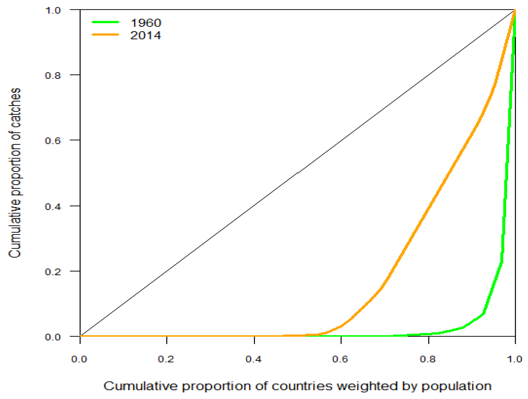
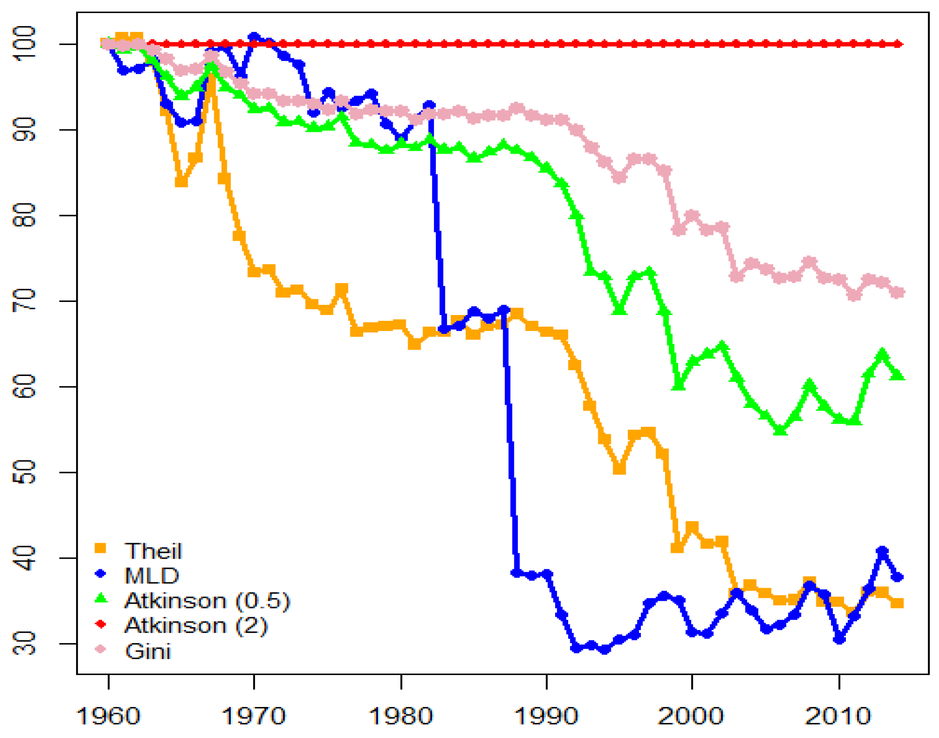
3.4. Global Inequality in Catches

The evolution of the Lorenz curves for the distribution of catches shows that countries in the middle and upper parts of the distribution have increased their share in total catches, bringing the curve closer to the diagonal (Figure 4). Thus, it can be unambiguously claimed that the 2014 distribution is more equal than the 1960 distribution.

In addition to this graphic result, we are interested in quantifying the inequality in the international distribution of fisheries resources from 1960 to 2014. In particular, we calculated the Gini index, the Atkinson index with parameters 2 (A(2)) and 0.5 (A(0.5)), the Theil index and the Mean Logarithmic Deviation (MLD). Figure 5 illustrates the results. To provide a clearer view of the multiple paths of inequality suggested by the indexes, the inequality values for 1960 are taken as a reference and normalized to 100. Positive and negative fluctuations of inequality place indexes above and below 100, respectively. This enables the magnitude of the changes in inequality to be compared over the period analyzed.

Several features can be highlighted from the evolution of the inequality indexes (Figure 5). As previously seen through the evolution of the Lorenz curves, the distribution of catches across countries has become more homogeneous during the period analyzed. In particular, it can be observed that inequality in the distribution of catches has decreased between 29% and 65% from 1960 to 2014, depending on the index. Instead of being monotonic, the evolution of indexes experiences fluctuations from one year to another. Nevertheless, three periods can be clearly distinguished. From 1960 to the mid-1980s, inequality follows a decreasing trend (the largest variation found in the indexes during this period does not represent more than 34% of the initial level). A few years after the recognition of EEZs by the UNCLOS in 1982 [7], the decreasing trend in inequality intensifies. This change in the behavior of inequality seems reasonable once the EEZ came into effect, as many fleets operating in the EEZ of foreign countries had to move toward other stocks, in most cases, located in high seas. This was especially the case of the fisheries from the US and Canada and to a considerable lesser extent those fisheries in Northwest Africa [48]. These movements decreased inequality as high seas areas became exploited by more countries. During the last stage, 2000–2014, inequality continues decreasing, but more smoothly. This is due to the stability observed in catches (see Figure 1) mainly produced by the boom in aquaculture in this period [49].

Another remarkable feature illustrated in Figure 5 is the differences observed between the indexes over time. With the exception of the A(2), all indexes show similar trends. In particular, the trend in A(2) distinguishes for being quite flat. This has also been observed in other studies analyzing distributional issues on environmental resources [27] and is due to the inherent characteristics of the Atkinson family of indexes. A(2) is an index which takes into close consideration the observations located at the bottom of the distribution. This implies that, in our case, the A(2) pays especial attention to countries with zero catches from high seas. Even though their proportion has decreased over the period analyzed, there is still a large amount of countries with zero catches. Thus, changes in the inequality when focusing on the bottom part of the catches distribution are negligible. In this sense, we do not consider that A(2) represents the equity in exploitation of fisheries resources well. The rest of the indexes show similar trends, but the differences among them are relevant from the quantitative viewpoint. The Gini index shows the smallest variation in inequality (apart from the A(2) index) over time, because it is very sensitive to changes in the part of the distribution with most observations, i.e., the low tail of the distribution, in our case. The differences observed in the trend of the Theil index and the MLD also reflect the inherent characteristics of this family of indexes. Both belong to the General Entropy family (Table 1), but the Theil index is more sensitive to changes in the upper tail than the MLD. This is why the former quantifies more inequality than the latter for the same distribution.

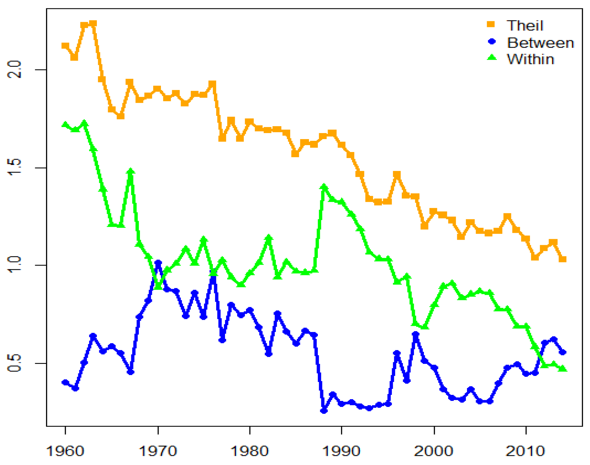
3.5. Decomposition of Inequality by Fishing Areas: Biology vs. Technology

The decomposability property of the Theil index allows calculating how much of the inequality observed in fishery catches can be explained by differences between fishing areas and how much by differences across countries operating within those areas. The between component would represent mostly the biological differences between the fishing areas (species, biodiversity, nutrients availability, temperature, climate conditions, etc.). The within component would represent the differences across the fleets fishing within the area. These differences may reflect the technological characteristics of the fleets (fishing gear, vessel size and power, and EEZ boundary), the fishermen capacities or the food preferences of population among countries. Since large dissimilarities in the fleets and fishermen capacity of countries are outlined in [1] and differences in the preferences for fish consumption are difficult to measure and may be overpassed by preferences for exporting fish, we associate this component of the inequality, roughly speaking, with technology.

Figure 6 illustrates the evolution of the total inequality and the between and within components of the inequality in the catches of countries from 1960 to 2014. For an easier comparison of the contributions of each component, these results are not normalized using the initial year as in Figure 5. There are two facts worth highlighting in Figure 6. On the one hand, we observe that inequality has reduced more than 33% in relative terms between 1960 and 2014. Since the maximum value of the Theil index is given by $Ln\left(n\right)$ being in our case $n=166$, we can say that in 1960 the inequality in the use of fishing resources was about 51% of the maximum inequality while in 2014 the inequality was about 18%.

On the other hand, Figure 6 shows that inequality in the high seas catches of countries has been mostly produced by differences within fishing areas during the period analyzed. That is, most of the inequality observed is due to the dissimilarity in the average catches between the fleets operating within the same area. This is in line with Sumaila and Teh [9], who found that only more industrialized countries can access and exploit high seas, being the least developed countries limited to the nearest areas. Nevertheless, the gap between the between and the within components narrows over time to the point that the between component exceeds the within component in the last years of the sample. This evolution reflects the technological catching up across countries.

Table 4. Proportion of inequality from between and within fishing areas.

Year	Within	Between
1960	80.89	19.11
1970	46.57	53.43
1980	55.38	44.62
1990	81.94	18.06
2000	62.50	37.50
2010	60.68	39.32
2014	45.71	54.29

quantifies the Theil decomposition for the key years in percentage terms. As shown in Figure 6, the inequality observed seems to have been mainly motivated by inequality among countries fishing within the same area (between 45% and 82% of the total inequality is explained by this component). Although its initial contribution seems to maintain at a lower levels during the first decades, the within inequality experiences a noticeable increase in the 1990s. This spike might be explained by the implementation of the EEZ in the 1980s. Due to the new legislation, many countries lost their free access to coastal waters previously exploited. In the short term, these countries may have decided to keep their levels of catches by expanding their fishing activities to high seas areas. This sudden movement of the fleets might have result in a quasi-random spread of vessels around global waters, which decreases the biological inequality. At the same time, countries enforced to leave the coastal waters may not have such productive fleets to fish in high seas areas. Consequently, there is more heterogeneity in the fleets of these areas, resulting in the observed increase in within inequality. Over the last decades of the period analyzed, the percentage contribution of the within inequality has decreased, which reflects the greater reliance of more countries on high seas fisheries and their catching up on fishing technology. Indeed, in the last years, the within inequality has overpassed the between inequality, which reflects that catches dissimilarities are rather generated by the idiosyncrasies of the areas exploited.

When decomposing the Theil index into between and within inequality, we can compute the contribution of each area to the latter component. Figure 7 shows the contribution of fishing areas to the within component. Note that a small (large) contribution by a particular area indicates that the distribution of catches among the countries fishing within this area is quite homogeneous (heterogeneous).

In aggregate terms, Figure 7 shows that the Pacific has been responsible for around half of the within inequality observed during the whole period. The Atlantic, which generated one third of the initial within inequality, presents half of its initial share by the end of the period. On the contrary, the Indian Ocean has slightly increased its percentage contribution to within inequality during the period analyzed. Even though there is not a single area standing out above the rest, noticeable changes have occurred from 1960 to 2014.

On the one hand, areas such as the Western Central Pacific, the Southeast Pacific, the Eastern Indian Ocean, the Antarctic Atlantic or the Eastern Central Atlantic have increased their percentage contribution to within inequality. Within the Western Central Pacific, the concentration of catches seems to have decreased from 1960 to 2014. In the beginning of the period, around 84% of the catches were held by Japan, which represented only 4% of the population of this area. At the end, the largest fisher in this area are Indonesia (with 21% of the catches) and the Republic of Korea (with 20% of the catches), representing 13% and 3% of the population, respectively. Despite this decrease in the percentage concentration, the rise in the catches of this area (Figure 3) has motivated such enlargement of the contribution of the within contribution. In the Southeast Pacific, Japan represented 85% of the initial catches, with less than 2% of the population. By the end of the period analyzed, the major fishing entity in this area is Ecuador with 50% of the catches and approximately 4% of the population. In this case, it can also be observed that, although there has been a noticeable decrease in the concentration of percentage catches in this area, the increase in the absolute levels of catches (Figure 3) results in an increase in the contribution of this area to within inequality. Regarding the Eastern Indian Ocean, Japan initially was responsible of all the catches in this area, representing less than 8% of the population. In 2014, Spain becomes the major fishing entity with one third of the catches and 4% of the population of the area. Again, the increase in catches has produced the increased observed in the within inequality despite the fall in the concentration of percentage catches. The increase in the within contribution of the Antarctic Atlantic is explained by the fact that this area started to be exploited during the period analyzed. Within the Eastern Central Atlantic, there has been also a decrease in the concentration of percentage catches. In particular, the initial major fishing entity was Malta, with 71% of the catches of this area and 0.2% of its population. Ghana constitutes the largest final fishing entity of this area, representing 24% of the catches and 10% of the population in this area. The boost in the absolute catches of this area (Figure 3) motivates the increase in its contribution to the within inequality.

On the other hand, areas such as the Northwest Pacific, the Southwest Atlantic or the Northern Atlantic have decreased their share in the within inequality. In the Northwest Pacific, the decrease in the concentration of percentage catches is noticeable, which may explain the decrease in its contribution to within inequality. Particularly, it can be found that this area was initially mostly exploited by Japan (92%), a country which only accounted for 6% of the population. Finally, Indonesia holds the largest amount of catches (32%) while only represents 12% of the population. In the case of the Southwest Atlantic, the concentration of major percentage catches seems to maintain over the period analyzed. Nevertheless, the decrease observed in the catches of this area (Figure 3) explains the reduction in the within contribution of this area. While the concentration of the percentage catches of the major fishing entities in the Northeast Atlantic decreases, that in the Northwest Atlantic increases. Catches in both of these areas decrease, contributing to the decrease in the within inequality in Northeast Atlantic and producing the negative variation in the within inequality of the Northwest Atlantic.

4. Discussion and Conclusions

While perfectly equal distributions may threat the target of resources conservation by allowing numerous agents to exploit a limited resource, sustainability policies are also compromised by very unequal distributions, where less benefited agents may not be as prompt to burden with the same costs [50,51,52]. This analysis aims to help policy makers through the illustration of the fishery resources distribution, which may contribute to know the general predisposition of countries to participate in a common conservation plan.

It is well known that fishery catches have traditionally been concentrated in a few countries and fishing areas. This article quantifies the distributional issues that emerge when fisheries exploitation is analyzed over time by applying the inequality metrics used in social science.

Other articles have also used inequality metrics to study different issues arising in fisheries economics. Sumaila et al. [53] used the Gini index to quantify the distributional effects on profits of the closure of the high seas to fishing. The Gini index was also used by Da Rocha and Sempere [54] to measure the redistributive effects of restricting the tradability of individual transferable quotas. Bellanger et al. [38] used the Theil index and its decomposability property to determine the distributional effects of various quota allocation systems among producer organizations. Unlike these articles, our study does not set out to assess the distributional effect of a particular management fisheries policy, but rather to show the unequal use of worldwide fisheries resources over time.

We address the distributional analysis of marine resources as a global common considering catches exclusively from high seas. Catches from the EEZs are not considered a common resource because, from the legal point of view, they are fully under the national jurisdiction of a particular state [7]. In this context, all inequality indexes confirm that the use of fishing resource is very unequal across countries. However, this use has become more equal over time, with inequality decreasing by between 29% and 65% from 1960 to 2014. This study also shows that, when the geographical origin of the catches is taken into account, until 2000 more than three quarters of the inequality observed in fishing catches is due to technological and fishermen capacity differences across the countries operating within fishing areas. This trend is in line with the results of Sumaila et al. [53], who found that the number of countries fishing in shared areas has doubled from 1950 to 2006. However, this percentage has decreased by more than 35% in the last few decades, reflecting the greater reliance of more countries on high seas fisheries and their catching up on fishing technology. In fact, in the last years of the sample, the between component has exceeded the within component reflecting the fact that the biological differences between the fishing areas may have widened.

All these findings are very relevant from the policy viewpoint. Policies seeking to ensure the sustainability of marine resources have to take these equity issues into account in the management of the international high seas [9]. Jointly with the distribution of fishing effort, the catches of the areas reported in this analysis may provide an idea on whether fishing areas can be further exploited or need to be preserved from their unsustainable exploitation, helping countries to homogenize their catches by redirecting their fishing activity to more productive areas. Nonetheless, an egalitarian use of the fishing resources has to be aligned with other actions that guarantee an equitable use. Other factors such as dependence (i.e., food security), traditional access to the resource or development needs also have to be taken into account for the sustainability of the resource [8,55,56]. These recommendations are also aligned with the awareness campaigns that promote the sustainability of fisheries by advocating for an eco-labeling of fish that includes information such as the origin of the fish [57,58] or the way in which it has been caught [59].

The search for an egalitarian use of the fishing resources is compatible with the view of the sea as common heritage of mankind rather than a free and open access resource [60,61]. Some proposals for protecting fishing resources consider the closure of the high seas [53], the creation of (no-take) marine reserves [62,63,64], or the zoning of the entire oceans, not just the land margin [65]. Our result are a support for all these proposals as long as the distributional effects are taken into account in the analysis, as Sumaila et al. [53] did for the case of the high seas closure.

One of the shortcomings of our analysis is that it does not incorporate the management frameworks. Our approach quantifies the inequality of the use of fisheries resource along time but it is not able to explain the reasons of this inequality. High seas are governed by the RFMOs with different management powers to set rules that condition the fishing decisions of the fleets. Even though some of the measures adopted for the RFMOs do not advocate the equal exploitation of the stocks fisheries, this is the case of the European Common Fisheries Policy that allocates quotas among the state members according to the Principle of Relative Stability, which takes into account the historical catch records instead of their population [66,67]. In the same line, our approach it is not able a priori to take explicitly into account the biological differences of the fishing areas; however, it is able to distinguish a posteriori how much of the inequality observed in fishing catches can be explained by differences between fishing areas, which we take mainly as biological differences.

Further research on the availability of fishery substitutes (aquaculture), jointly with an economic valuation of the profits obtained from the commercialization of the catches (including exports), would provide more precise information on the initial willingness of countries to participate in international conservation plans for fisheries. Our analysis skips from the fact that some countries export most of their catches and import other fish products due to the food preference of their people. For instance, Japan exported 16% of fish captured in 2016, according to the FAO data. In contrast, United States exported 31% of fish captured that same year [68,69]. Nonetheless, analyzing the exploitation patterns, instead of consumption patters, allows us to account for that part of the resource that is captured and exported to other countries. We are implicitly assuming that local population benefits from these exports. From an economic perspective, it would be of interest to quantify the inequality in the distribution of the profits derived from exploitation of the fisheries resources. In [19], the authors analyzed the profits of several countries obtained very recently from exploitation of high seas fisheries. Some studies (e.g., [70,71]) focus on the distribution of profits across agents from specific fisheries but, as far as we know, no studies analyze the distribution of the profits from fishing between countries.

Inequality metrics can be applied to many other distributional concerns of interest in fisheries. One of the shortcomings of our analysis is that catches are taken as a pool without distinguish by species or taxon or by the type of vessel used for harvesting. However, it could be interesting to analyze the distribution of catches by (groups of) species or by types of vessels instead of geographical areas.

Finally, it is worth noting that the catch data used in this study come from the reconstructed series by Pauly and Zeller [36] in the Sea Around Us project [35]. Some studies (e.g., [72]) show that data reported to the FAO in recent years by some countries such as China and Myanmar are unreliable because increases in catches may be politically expedient. Moreover, Pauly and Zeller [73] highlighted the importance of retroactive corrections in FAO time series to avoid a “presentist bias”. Researchers from the FAO refute these criticisms, although they are open to new research that may help to improve their statistical data on fisheries [74]. In this context of discussion, we have repeated our analysis with the FAO data for the case of the global catches. Results with the FAO data are qualitatively similar to those presented in this article.

References

1. FAO. The State of World Fisheries and Aquaculture 2018. Meeting the Sustainable Development Goals; Food and Agriculture Organization of the United Nations, Fisheries and Aquaculture Department: Rome, Italy, 2018. [Google Scholar]
2. CBD (Ed.) Aichi Biodiversity Targets. Convention Biological Diversity Strategic Plan Biodiversity 2011–2020; UNEP: Montreal, QC, Canada, 2010. [Google Scholar]
3. UN. Transforming Our World: The 2030 Agenda for Sustainable Development; United Nations General Assembly: New York, NY, USA, 2015. [Google Scholar]
4. Perissi, I.; Bardi, U.; El Asmar, T.; Lavacchi, A. Dynamic Patterns of Overexploitation in Fisheries. Ecol. Model. 2017, 359, 285–292. [Google Scholar] [CrossRef]
5. FAO. The State of World Fisheries and Aquaculture 2016: Contribution to Food Security and Nutrition for All; Food and Agriculture Organization of the United Nations, Fisheries and Aquaculture Department: Rome, Italy, 2016. [Google Scholar]
6. Grotius, H. Mare Liberum; Lodewijk Elzevir: Leuven, Belgium, 1609. [Google Scholar]
7. UN General Assembly. United Nations Convention on the Law of the Sea; United Nations General Assembly: Montego Bay, Jamaica, 1982. [Google Scholar]
8. Schiller, L.; Bailley, M.; Jacquet, J.; Sala, E. High seas fisheries play a negligible role in addressing global food security. Sci. Adv. 2018, 4, eaat8351. [Google Scholar] [CrossRef] [Green Version]
9. Sumaila, U.; Teh, L. Trends in Global Shared Fisheries. Mar. Ecol. Prog. Ser. 2015, 530, 243–254. [Google Scholar]
10. Jackson, J.; Kirby, M.; Berger, W.; Bjorndal, K.; Botsford, L.; Bourque, W.; Bradbury, R.; Cooke, R.; Erlandson, J.; Estes, J.; et al. Historical overfishing and the recent collapse of coastale cosystems. Science 2001, 293, 629–638. [Google Scholar] [CrossRef]
11. Pauly, J.; Christensen, V.; Guénette, S.; Pitcher, T.; Sumaila, U.; Walters, C.; Watson, R.; Zeller, D. Towards sustainability in world fisheries. Nature 2002, 418, 685–695. [Google Scholar] [CrossRef]
12. Hegland, T.; Raakjaer, J. Recovery Plans and the Balancing of Fishing Capacity and Fishing Possibilities: Path Dependence in the Common Fisheries Policy. In Making Fisheries Management Work. Reviews: Methods and Technologies in Fish Biology and Fisheries; Gezelius, S., Raakjaer, J., Eds.; Springer: Dordrecht, The Netherlands, 2008; Volume 8. [Google Scholar]
13. Da Rocha, J.; Gutiérrez, M. Lessons from the long-term management plan for northern hake: Could the economic assessment have accepted it? Ices J. Mar. Sci. 2011, 68, 1937–1941. [Google Scholar] [CrossRef]
14. Cardinale, M.; Dorner, H.; Abella, A.; Andersen, J.; Casey, J.; Doring, R.; Kirkegaard, E.; Motova, A.; Anderson, J.; Simmonds, E.; et al. Rebuilding EU fish stocks and fisheries, a process under way? Mar Policy 2013, 39, 43–52. [Google Scholar] [CrossRef]
15. USFWS. Report to Congress, Endangered and Threatened Species Recovery Program, 1996; US Fish and Wildlife Service, Government Printing Office: Washington, DC, USA, 1999.
16. Palomares, M.; Pauly, D. Coastal fisheries: The past, present and possible futures. In Coasts and Estuaries; Elsevier: Amsterdam, The Netherlands, 2019. [Google Scholar]
17. Roberts, C. Deep impact: The rising toll of fishing in the deep sea. Trends Ecol. Evol. 2002, 17, 242–245. [Google Scholar] [CrossRef]
18. Morato, T.; Watson, R.; Pitcher, T.; Pauly, D. Fishing down the deep. Fish Fish. 2006, 7, 24–34. [Google Scholar] [CrossRef]
19. Sala, E.; Mayorga, J.; Costello, C.; Kroodsma, D.; Palomares, M.; Pauly, D.; Sumaila, U.; Zeller, D. The economics of fishing the high seas. Sci. Adv. 2018, 4, eaat2504. [Google Scholar] [CrossRef] [Green Version]
20. Cullis-Suzuki, S.; Pauly, P. Failing thehighseas: A global evaluation of regional fisheries management organizations. Mar. Policy 2010, 34, 1036–1042. [Google Scholar] [CrossRef]
21. Azar, C.; Holmberg, J.; Lindgren, K. Socio-ecological indicators for sustainability. Ecol. Econ. 1996, 18, 89–112. [Google Scholar] [CrossRef]
22. Hori, S. Member state commitments and international environmental regimes: Can appeals to social norms strengthen flexible agreements? Environ. Sci. Policy 2015, 54, 263–267. [Google Scholar] [CrossRef]
23. Owusu, K.; Kulesz, M.; Merico, A. Extraction Behaviour and Income Inequalities Resulting from a Common Pool Resource Exploitation. Sustainability 2019, 11, 536. [Google Scholar] [CrossRef]
24. Drupp, M.A.; Meya, J.N.; Baumgärtner, S.; Quaas, M.F. Economic Inequality and the Value of Nature. Ecol. Econ. 2018, 150, 340–345. [Google Scholar] [CrossRef] [Green Version]
25. Fabinyi, M.; Foale, S.; Macintyre, M. Managing Inequality or Managing Stocks? An Ethnographic Perspective on the Governance of Small-Scale Fisheries. Fish Fish. 2015, 16, 471–485. [Google Scholar] [CrossRef]
26. Padilla, E.; Serrano, A. Inequality in CO2 emissions across countries and its relationship with income inequality: A distributive approach. Energy Policy 2006, 34, 1762–1772. [Google Scholar] [CrossRef]
27. Duro, J. On the Automatic Application of Inequality Indexes in the Analysis of the International Distribution of Environmental Indicators. Ecol. Econ. 2012, 76, 1–7. [Google Scholar] [CrossRef]
28. Farrell, N. What Factors Drive Inequalities in Carbon Tax Incidence? Decomposing Socioeconomic Inequalities in Carbon Tax Incidence in Ireland. Ecol. Econ. 2017, 142, 31–45. [Google Scholar] [CrossRef] [Green Version]
29. Azimi, M.; Feng, F.; Yang, Y. Air Pollution Inequality and Its Sources in SO2 and NOX Emissions among Chinese Provinces from 2006 to 2015. Sustainability 2018, 10, 367. [Google Scholar] [CrossRef]
30. White, T. Sharing resources: The global distribution of the Ecological Footprint. Ecol. Econ. 2007, 64, 402–410. [Google Scholar] [CrossRef]
31. Alcántara, V.; Duro, J. Inequality of energy intensity across OECD countries: A note. Energy Policy 2004, 32, 1257–1260. [Google Scholar] [CrossRef]
32. Duro, J.; Padilla, E. Inequality across countries in energy intensity: An analysis of the role of energy transformation and final energy consumption. Energy Econ. 2011, 33, 474–479. [Google Scholar] [CrossRef]
33. Li, R.; Jiang, X. Inequality of Carbon Intensity: Empirical Analysis of China 2000–2014. Sustainability 2017, 9, 711. [Google Scholar] [CrossRef]
34. Duro, J.; Schaffartzik, A.; Krausmann, F. Metabolic Inequality and Its Impact on Efficient Contraction and Convergence of International Material Resource Use. Ecol. Econ. 2018, 145, 430–440. [Google Scholar] [CrossRef]
35. SeaAroundUs. Available online: http://www.seaaroundus.org (accessed on 8 March 2019).
36. Pauly, D.; Zeller, D. (Eds.) Sea Around Us Concepts, Design and Data (seaaroundus.org); University of British Columbia: Vancouver, BC, Canada, 2015. [Google Scholar]
37. World Bank. Data Catalog; The World Bank Group: Washington, DC, USA, 2019. [Google Scholar]
38. Bellanger, M.; Macher, C.; Guyader, O. A new approach to determine the distributional effects of quota management in fisheries. Fish. Res. 2016, 181, 116–126. [Google Scholar] [CrossRef] [Green Version]
39. Lorenz, M. Methods of Measuring the Concentration of Wealth. Am. Stat. Assoc. 1905, 9, 209–219. [Google Scholar] [CrossRef]
40. Theil, H. Economics and Information Theory; North Holland: Amsterdam, The Netherlands, 1967. [Google Scholar]
41. Atkinson, A. On the Measurement of Inequality. J. Econ. Theory 1970, 3, 244–263. [Google Scholar] [CrossRef]
42. Cowell, F. Measuring inequality. In LSE Perspectives in Economic Analysis; Oxford University Press: Oxford, UK, 2009. [Google Scholar]
43. Allison, P. Measures of Inequality. Am. Sociol. Rev. 1978, 43, 865–880. [Google Scholar] [CrossRef]
44. Gini, C. Variabilitá e mutabilitá, contributo allo studio delle distribución e relazioni statistiche; Tipografia di Paolo Cuppin: Bologna, Italy, 1912. [Google Scholar]
45. Shorrocks, A.F. The Class of Additively Decomposable Inequality Measures. Econometrica 1980, 48, 613–625. [Google Scholar] [CrossRef]
46. Shorrocks, A.F. Inequality Decomposition by Population Subgroups. Econometrica 1984, 52, 1369–1385. [Google Scholar] [CrossRef]
47. Bellù, L.; Liberati, P. Describing income inequality. Theil index and entropy class indexes. FAO EasyPol 2006, 51. [Google Scholar]
48. Pauly, D. Beyond duplicity and ignorance in global fisheries. Sci. Mar. 2009, 73, 215–224. [Google Scholar] [CrossRef] [Green Version]
49. Nadarajah, S.; Flaaten, O. Global aquaculture growth and institutional quality. Mar. Policy 2017, 84, 142–151. [Google Scholar] [CrossRef] [Green Version]
50. Halpern, B.; Klein, C.; Brown, C.; Beger, M.; Grantham, H.; Mangubhai, S.; Ruckelshaus, M.; Tulloch, V.; Watts, M.; White, C.; et al. Achieving the triple bottom line in the face of inherent trade-offs among social equity, economic return and conservation. Proc. Natl. Acad. Sci. USA 2013, 110, 6229–6234. [Google Scholar] [CrossRef] [PubMed]
51. Manach, F.L.; Andriamahefazafy, M.; Harper, S.; Harris, A.; Hosch, G.; Lange, G.M.; Zeller, D.; Sumaila, U.R. Who gets what? Developing a more equitable framework for EU fishing agreements. Mar. Policy 2013, 38, 257–266. [Google Scholar] [CrossRef]
52. Klein, C.; McKinnon, M.; Wright, B.; Possingham, H.; Halpern, B. Social equity and the probability of success of biodiversity conservation. Glob. Environ. Chang. 2015, 35, 299–306. [Google Scholar] [CrossRef] [Green Version]
53. Sumaila, U.R.; Lam, V.W.Y.; Miller, D.D.; Teh, L.; Watson, R.A.; Zeller, D.; Cheung, W.W.L.; Côté, I.M.; Rogers, A.D.; Roberts, C.; et al. Winners and losers in a world where the high seas is closed to fishing. Sci. Rep. 2015, 5, 8481. [Google Scholar] [CrossRef]
54. Da Rocha, J.M.; Sempere, J. ITQs, Firm Dynamics and Wealth Distribution: Does Full Tradability Increase Inequality? Environ. Resour. Econ. 2016, 68, 249–273. [Google Scholar] [CrossRef] [Green Version]
55. Belton, B.; Thilsted, S.H. Fisheries in transition: Food and nutrition security implications for the global South. Glob. Food Secur. 2014, 3, 59–66. [Google Scholar] [CrossRef] [Green Version]
56. Levine, A.S.; Richmond, L.; Lopez-Carr, D. Marine resource management: Culture, livelihoods, and governance. Appl. Geogr. 2015, 59, 56–59. [Google Scholar] [CrossRef]
57. Bonanomi, S.; Colombelli, A.; Malvarosa, L.; Cozzolino, M.; Sala, A. Towards the Introduction of Sustainable Fishery Products: The Bid of a Major Italian Retailer. Sustainability 2017, 9, 438. [Google Scholar] [CrossRef]
58. Kim, B.T.; Lee, M.K. Consumer Preference for Eco-Labeled Seafood in Korea. Sustainability 2018, 10, 3276. [Google Scholar] [CrossRef]
59. Onofri, L.; Accadia, P.; Ubeda, P.; Gutiérrez, M.; Sabatella, E.; Maynou, F. On the Economic Nature of Consumers’ Willingness to Pay for Selective and Sustainable Fishery: A Comparative Empirical Study. Sci. Mar. 2018, 82, 91–96. [Google Scholar] [CrossRef]
60. Schrijver, N. Managing the global commons: common good or common sink? Third World Q. 2016, 37, 1252–1267. [Google Scholar] [CrossRef]
61. Stel, J. Ocean Space and Sustainability. In Sustainability Science; Heinrichs, H., Martens, P., Michelsen, G.A.W., Eds.; Springer: Dordrecht, The Netherlands, 2016; Chapter 16; pp. 193–202. [Google Scholar] [CrossRef]
62. Roberts, C.; Bohnsack, J.; Gell, F.; Hawkings, J.; Goodridge, R. Effects of marine reserves on adjacent fisheries. Science 2001, 294, 1920–1923. [Google Scholar] [CrossRef]
63. Gell, F.; Roberts, C. Benefits beyond boundaries: The fishery effects of marine reserves. Trends Ecol. Evol. 2003, 18, 448–455. [Google Scholar] [CrossRef]
64. Sala, E.; Giakoumi, S. No-take marine reserves are the most effective protected areas in the ocean. Ices J. Mar. Sci. 2017, 75, 1166–1168. [Google Scholar] [CrossRef] [Green Version]
65. Russ, G.R.; Zeller, D.C. From Mare Liberum to Mare Reservarum. Mar. Policy 2003, 27, 75–78. [Google Scholar] [CrossRef]
66. Da-Rocha, J.M.; Gutiérrez, M.J. The optimality of the Common Fisheries Policy: The Northern Stock of Hake. Span. Econ. Rev. 2006, 8, 1–21. [Google Scholar] [CrossRef]
67. Hoefnagel, E.; de Vos, B.; Buisman, E. Quota swapping, relative stability, and transparency. Mar. Policy 2015, 57, 111–119. [Google Scholar] [CrossRef]
68. FAO. Global Capture Production; Food and Agriculture Organization of the United Nations. Fisheries and Aquaculture Department: Rome, Italy, 2019. [Google Scholar]
69. FAO. Fishery Commodities and Trade; Food and Agriculture Organization of the United Nations. Fisheries and Aquaculture Department: Rome, Italy, 2019. [Google Scholar]
70. Pascoe, S.; Giles, N.; Coglan, L. Extracting fishery economic performance information from quota trading data. Mar. Policy 2019, 102, 61–67. [Google Scholar] [CrossRef]
71. Rodrigues, A.; Abdallah, P.; Gasalla, M. Cost structure and financial performance of marine commercial fisheries in the South Brazil Bight. Fish. Res. 2019, 210, 162–174. [Google Scholar] [CrossRef]
72. Pauly, D.; Zeller, D. Comments on FAOs State of World Fisheries and Aquaculture (SOFIA 2016). Mar. Policy 2017, 77, 176–181. [Google Scholar] [CrossRef]
73. Pauly, D.; Zeller, D. The best catch data that can possibly be? Rejoinder to Ye et al. “FAO’s statistic data and sustainability of fisheries and aquaculture”. Mar. Policy 2017, 81, 406–410. [Google Scholar] [CrossRef]
74. Ye, Y.; Barange, M.; Beveridge, M.; Garibaldi, L.; Gutierrez, N.; Anganuzzi, A.; Taconet, M. FAO’s statistic data and sustainability of fisheries and aquaculture: Comments on Pauly and Zeller (2017). Mar. Policy 2017, 81, 401–405. [Google Scholar] [CrossRef]
Figure 1. Evolution of high seas catches and population.
Sustainability 11 03133 g001
Figure 2. Distribution of high seas catches and population by countries: (a) 1960; and (b) 2014.
Sustainability 11 03133 g002
Figure 3. Contribution of fishing areas to high seas catches and population. “Others” represent fishing areas whose global catches and population were below 1 % in 1960 and 2014.
Sustainability 11 03133 g003
Figure 4. Lorenz curves.
Sustainability 11 03133 g004
Figure 5. Evolution of inequality.
Sustainability 11 03133 g005
Figure 6. Between and within inequality decomposition of the Theil index.
Sustainability 11 03133 g006
Figure 7. Contribution of fishing areas to the within inequality. “Others” represents fishing areas whose contribution was below 1 % in the years shown.
Sustainability 11 03133 g007