The Effects of the Layouts of Vegetation and Wind Flow in an Apartment Housing Complex to Mitigate Outdoor Microclimate Air Temperature

Abstract

Previous studies have demonstrated that vegetation and increased air flow can mitigate air temperature by employing numerical models, satellite remote sensing or Computational Fluid Dynamics simulations. This study aimed to examine how layouts of vegetation space and wind flow affect microclimate air temperature, which directly affects city dwellers’ thermal comfort in summer, in a real apartment housing complex in Seoul, South Korea. To do this, a Reynolds-averaged Navier–Stokes model was utilized, combined with a finite volume method CFD simulation, and which measured transpirational cooling effects of vegetation by comprehensively considering air humidity by transpiration, as well as wind flow of the surroundings, to reflect actual conditions of urban environments. Based on the computational model, nine scenarios including elevated building designs were simulated. The findings of this study are as follows: First, different layouts of vegetation and wind flow clearly affected microclimate air temperature in the housing complex. Second, when the total area of vegetation was the same, it was more effective to reduce air temperature by placing it in small units rather than concentrating it in one place, and placing small vegetation spaces close to buildings was better than locating them between buildings. Third, it was apparent that an elevated space works as a wind path, leading to increasing wind velocity. However, it was revealed that wind flow does not always positively affect hot temperatures.

1. Introduction

Summer temperatures are expected to continue rising worldwide due to the presence of global warming and climate change, leading to negative effects on human environments and health. Urban areas, especially, are facing more serious conditions because of the urban heat island (UHI) effect [1]. In a city, man-made structures, such as buildings and roads covered with asphalt hinder ventilation and trap solar radiation, in addition to diverse urban activities producing heat and air pollution, increase air temperature higher than in rural or suburban areas [2,3].

Seoul, the capital of the Republic of Korea, is struggling with heat waves in summer months, too. According to a research report by the Seoul Institute, mean summer temperatures over the past ten years have increased 1.8 °C compared to temperatures one hundred years ago, and the highest temperature last year, 2018, reached 39.6 °C, which broke the previous record held for 111 years [4]. The report anticipates that this trend will continue to be exacerbated, by which many people in Seoul will be adversely affected [4]. To cope with this issue, the Seoul Metropolitan Government has implemented UHI mitigation strategies including the expansion of vegetated areas, open water surfaces, cool paving materials, and wind corridors [5]. These strategies help reduce air temperatures by increasing urban albedo reflecting solar radiation, evaporation absorbing heat, and air flow for ventilation. A number of previous studies have also broadly explored the roles of albedo [6,7], vegetation [8,9], and air flow [5,10] to moderate air temperature at the microclimate level, as well as in cases of the UHI effect.

Among them, the main mechanism for vegetation’s role in cooling air temperatures has been well identified as having two aspects: shading and evapotranspiration [8,11]. Berry et al. [12] showed that shading can decrease ambient air temperature by 1 °C and Georgi et al. [13] demonstrated 3.1 °C reduction via plant evapotranspiration. Zhang et al. estimated that vegetation cooling effect reduced the air condition demand by 3.09 × 108 kWh which takes up 60% of net cooling energy usage in Beijing [14].

Many studies also showed that increasing air flow mitigates air temperature. Choi et al. [5] suggested wind corridors, which can mitigate urban heat by stimulating air flow or ventilation, leading to shorter durations of high air temperatures. They also demonstrated that urban porosity can increase urban ventilation performance by creating more spaces for wind corridors, which results in ameliorating pedestrian thermal discomfort [5]. Bernard et al. [15] considered vegetation and wind by suggesting design directions for a park and its surrounding urban morphology, in which parks in cities function as cool air drainage. Bae and Song [16] concluded that wind flow in association with vegetation positively affects heat mitigation in a housing complex.

Computer fluid dynamic (CDF) approaches were used to evaluate wind flow around buildings for the first time in the 1970s [17,18]. In the following decades, there were more studies aimed at outdoor environments for multiple building configurations. Ashie and Kono [19] and Tominaga et al. [20] utilized k-ε models to investigate the urban outdoor thermal environment for mitigating the microclimate. Liu and Niu et al. [21,22] analyzed the thermal comfort condition underneath an elevated building by using the measured thermal parameters and simulated wind velocity. The sensitivities for a large eddy simulation (LES) model and a delayed detached eddy simulation (DDES) model were tested in an idealized building array by Liu et al. [23] and Liu and Niu [24].

In addition, there have been several studies which have analyzed how different allocations of vegetation impact the cooling effect through numerical models, satellite remote sensing or CFD simulations. Hong et al. [25] investigated the outdoor thermal conditions between two kinds of green space allocations in four types of building layouts by using the Simulation Platform for Outdoor Thermal Environment (SPOTE) databases and Li et al. [26] examined the cooling effects of five scenarios of green space patterns in an ENVI-met model. However, the remote sensing could only achieve coarse results and the ENVI-met model had the limitation of a low accuracy algorithm, although it used the software database to simulate environments. Especially, these studies did not consider the different design possibilities of elevated spaces and vegetation distribution in an actual urban environment. Gromke et al. [11] developed a simulation method based on ANSYS Fluent to analyze the volumetric cooling effect of vegetation by considering the aerodynamics and other vegetative measures under a real urban street canyon in Arnhem, Netherlands. The ANSYS Fluent adopted the finite volume method and a high-precision algorithm, which was more selective for the turbulence models and could be freely adjusted for the mesh to meet all kinds of simulation demands including aerodynamics.

Yet, a limited number of studies have analyzed the transpirational cooling effects of vegetation by comprehensively considering the air humidity by transpiration, as well as the wind flow of the surroundings, in reflecting the actual conditions of urban environments. Furthermore, the relationship between the cooling effects, layouts of vegetation, and wind flow remain indistinct. For example, there has been no consensus regarding the cooling effects and spatial allocation of vegetation. Honjo et al. [27] suggested that smaller green areas with sufficient intervals are preferable for an effective cooling of surrounding areas by numerical estimate, while Wang et al. [28] argued that the fragmentation index of vegetation is positively related to land surface temperature.

This study attempts to take one step further. It aims to examine how layouts of vegetation space and wind flow affect microclimate air temperatures in an apartment housing complex. To do this, it used ANSYS Fluent, which is a more comprehensive finite volume method CFD simulation tool than that of previous studies, and considered not only transpirational cooling effects but also humidity produced by transpiration to allow us to compare the apparent temperature. Additionally, one of the main differences of this study from previous ones is that the case adopted for simulations was a real apartment housing complex in Seoul, Korea, and not just a generic model. Apartment housing is a dominant housing type in Seoul, which accounts for 58% of all housing units in Seoul [29]. Thus, design schemes for vegetation to ameliorate microclimate warming for apartment housing complexes will be very useful for urban inhabitants to cope with rising air temperatures in Seoul.

2. Methods

2.1. Study Area and Computational Model

The study area was a block in the “Acro-River Park Complex” located along the south of Han River in Seoul, Korea. It was built in 2016 and shows a recent design trend for an apartment housing complex in Korea, which is composed of tower-type and plat-type buildings. For this study, the middle unit of the complex was selected as a prototype cluster of the complex (Figure 1). The total area is approximately 14,710 m² and it consists of five buildings and a courtyard surrounded by four buildings (Figure 1).

Based on the CAD file of the complex and the field survey, the building and vegetation geometry of the study area was constructed in a computational model. The height of five apartment buildings in the study area varies from 45 m to 128 m (Figure 1), and to reflect the amount of vegetation inside the red line (exterior walls of the buildings in the study area) as seen in Figure 2, the vegetation area that consists of tall trees was measured based in a CAD drawing for a planting plan (Figure 2). From the measurement, the total vegetation area for simulations was decided at 1600 m². Then, it was modeled as a cubic configuration with a 6-m tall tree canopy and 1-m high bushes on the ground (Figure 3). Additionally, to explore the effect of wind flow and its relation to the location of vegetation, the elevated spaces were modeled based on the existing physical shape, 4 m tall and 8 m~14.8 m wide, reflecting the same size of one apartment unit in order to conform to the design (Figure 3 and Figure 4).

2.2. Computational Domain and Boundary Conditions

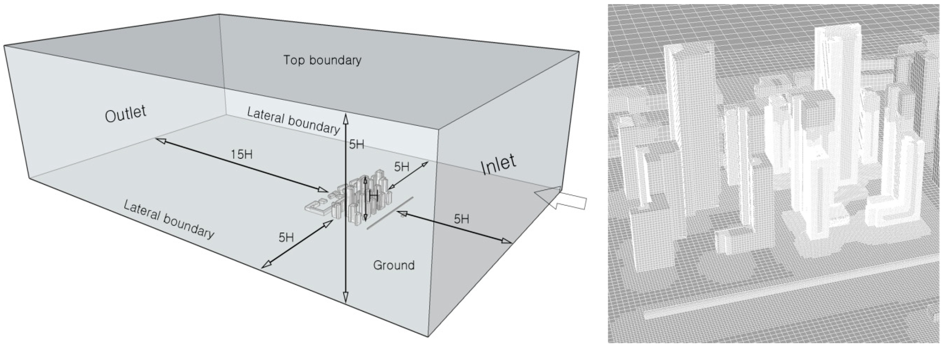
The complete CFD calculated domain, in which H (the height of the highest building) was 128 m, is shown in Figure 5 with the size according to the guidelines of Tominaga et al. [30]. An assembly meshing method was used, and the cells were refined within the boundary of the housing complex, and a standard wall function was adopted for Y+ value over 20 and under 400.

In this study, we compared a group of mesh to investigate the mesh independence, for which three kinds of mesh were defined by different cell growth rates. The coarse mesh had 2,163,194 cells and the fine mesh had 4,476,821 cells, while the finest mesh had 6,816,773 cells. Figure 6 displays that the results of the fine mesh and the finest mesh had a good convergence either in wind velocity or in air temperature. In terms of wind velocity, the maximum relative difference between the fine and finest mesh was roughly 1.03% at the 15 m level. For air temperature, the maximum relative difference between the fine and finest mesh was approximately 0.13% at the 2.5 m level. The t-test’s statistical significance at >98% showed that there was no difference between the fine mesh and the finest mesh. Hence, we can conclude that the fine mesh was able to provide sufficient accuracy, and in the next step, the number of mesh elements from 4 million to 5 million was adopted in the simulations.

Boundary conditions within the computational domain were set based on the weather data of 14:00 h local time, 2 August 2018, which was collected from the Korea Meteorological Office to estimate the hottest weather in one year. The observation station is 1.5 km from the complex. From the data, the inlet wind velocity = 1.8 m/s and turbulence intensity was approximately 5% at 16 m above ground from the north-west direction, with corresponding k = 121.5 and ε = 44.0. The inlet air temperature and relative humidity were set to 37.3 °C and 53.1%, respectively. Incident direct and diffuse solar radiation were 869.6 W∙m⁻² and 113.6 W∙m⁻², respectively, in terms of the position of Seoul and the simulated time. The vector of solar beams varied by time and the shading effect of buildings was considered, while the shading of vegetation was not. For buildings, wall thickness was set with 0.5 m to be simplified for outdoor simulations because the thickness of building walls can vary by height; that is, wall thickness with window ranges between 0.2 m through 0.3 m and that of walls without window ranges between 0.3 m through 0.4 m. Heat capacity = 970 J∙kg⁻¹ K⁻¹, thermal conductivity = 1.7 W∙m⁻¹ K⁻¹, and density = 2500 kg∙m⁻³ were specified. For the ground, heat capacity = 300 J∙kg⁻¹ K⁻¹, thermal conductivity = 1.1 W∙m⁻¹ K⁻¹, density = 2100 kg∙m⁻³ were set. Convective heat transfer occurs on outer building walls and ground surfaces. Air is heated by buildings and ground surfaces, but cooled by vegetation. All simulations were calculated by 10-core 20-thread computers (Intel Core i9-9900X @ 3.50 GHz), and simulated real-time was set to 1 h and the residuals were under 10⁻⁴.

To reflect the atmospheric boundary layer, the vertical profile of wind speed followed the log law [31]:

$$v\approx v_{ref}\cdot \frac{\ln \left(\frac{z}{z_0}\right)}{\ln \left(\frac{z_{ref}}{z_0}\right)}$$

(1)

where ν is the velocity to be calculated at height z, ν_ref is the known velocity at height z_ref; z is the height above ground level for velocity v; z_ref is the reference height where v_ref is known; and z₀, which is the roughness length in the current wind direction, was set at 0.8 for larger cities with tall buildings.

2.3. Numerical Model

This study employed a three-dimensional CFD simulation based on the finite volume method. The semi-implicit method for pressure-linked equations (SIMPLE) algorithm and second-order upwind scheme were selected to solve the conservation equations. Although k-ε turbulence models are widely used and acknowledged for engineering [32], there are still differences among several k-ε models. Santiago [33] and Tominaga [34] reported that a RNG k-ε model can reach better agreement with experiments on wind flow around buildings than standard k-ε and realizable k-ε models. Wu [35] examined the above models for estimating wind flow over a tree and compared them with wind tunnel experimental data from Mochida et al. [36], which demonstrated that the RNG k-ε model showed the highest accuracy. Liu et al. [22] also compared the wind velocity results between the RNG k-ε model and wind tunnel experiment, which showed a satisfied agreement. Here, although the DES model was closer to the experimental results, it spent more time computing. Therefore, this study adopted the RNG k-ε model for a high Reynolds number turbulence numerical simulation. This is a two-equations model based on Reynolds-Averaged Navier–Stokes (RANS) governing equations. The RANS simulation used the mean flow characteristics to describe turbulence instead of the detailed turbulence information.

2.4. Aerodynamical Reconstruction of Trees

The presence of trees can not only cause fluctuations in air flow but also decrease wind speed. Direct modeling of tree construction will result in excessively fine mesh, thereby leading to an unfavorable impact in calculating efficiency. Previous CFD simulations reflected the aerodynamic performance of a tree canopy by setting porous zones and introduced additional source terms in the governing equations [36,37]. Endalew et al. [38] constructed an even finer tree model as a real tree, but it reached a similar result with the porous zone tree model. It was also emphasized that a canopy plays the most important role whether in the configuration construct or transpiration rate [39]. Thus, since vegetation spaces are equivalent to the porous zone, only the tree canopy was modeled, and the leaf distribution inside was assumed to be uniform.

The aerodynamic effect of vegetation can be represented by introducing additional momentum source terms in the vegetation area. Thus, the additional terms (momentum source S_i, turbulence kinetic energy source S_k, and dissipation rate source S_ε) were added to the RANS governing equations. According to Green [40], Liu et al. [41], and Sanz [42], momentum source term S_i was defined as follows to reflect the momentum loss.

$$S_i=-\rho C_{d}LAD\left|U\right|U_i$$

(2)

where ρ is the density of air, C_d = 0.2 is the leaf drag coefficient; LAD is the leaf area density (m²∙m⁻³), referring to the characteristics of the vegetation foliage density; U_i is the velocity component of direction i; and U is the velocity magnitude inside the vegetation area.

Apart from momentum loss, the turbulence kinetic energy S_k and dissipation rate S_ε will also decrease because of the flow through the intricate canopy structure. Mochida et al. took the turbulence kinetic energy source S_k and dissipation rate Source S_ε from previous studies; and then, sorted them into four categories and optimized the parameter value for category A and category B as shown in

Table 1. Additional terms S_k and S_ε for the tree canopy model.

Category	Sk	Sε	Optimized Value
A	${\overline{u}}_i{S}_i$	${\mathrm{C}}_{p\epsilon 1}\frac{\epsilon }{k}{\overline{u}}_i{S}_i$	Cpε1 = 1.8
B	${\overline{u}}_i{S}_i-4\eta C_{d}LAD\left|{\overline{u}}_i\right|$	$\frac{\epsilon }{k}\left[C_{p\epsilon 1}\left({\overline{u}}_i{S}_i\right)-C_{p\epsilon 2}\left(4\eta C_{d}LAD\left|{\overline{u}}_i\right|\right)\right]$	Cpε1 = 1.8, Cpε2 = 1.5

[36]. In this study, category B [40,41] was applied.

S_k is the extra term added in the transport equation of k, S_ε is the extra term added in the transport equation of ε, η is the fraction of the area covered with trees, and C_pε1 and C_pε2 are regarded as model coefficients in turbulence modeling for prescribing the time scale of the process of energy dissipation in the canopy layer.

Regarding the revised vegetation model with source terms S_i, S_k, and S_ε (Equation (2) and Table 1), Gromke [11] and Moradpour [43] validated the above equations comparing them to field data from Amiro [44]. As a result, the maximum relative deviation of mean stream-wise velocity occurred at a height of approximately 40% and 30%, respectively, and the maximum relative deviation of kinematic Reynolds stress was about 20% and 42% each. Yet, in the other part of the canopy, good agreement of stream-wise velocity and kinematic Reynolds stress could be found with a correlation coefficient of over 0.90. Overall, it was concluded that the vegetation model was able to simulate the flow characteristics within the canopy. It can be said that the vegetation model was well validated based on these studies, so the user-defined function (UDF) file was compiled in C language, then interpreted into the CFD program.

2.5. Transpiration Heat Absorption and Water Release

As far as we know, there are only a few studies that have built the transpiration heat absorption model of vegetation and that were conducted by finite volume method CFD simulation. Two methodologies for vegetation modeling can be found. The first is to simulate vegetation into a solid block with a lower surface temperature [45]. This must assume that green vegetation has a lower leaf temperature than the ambient air [46], which might occur without direct solar radiation, and the main heat absorption process is conducted through heat convection as the temperature difference between leaf and air causes a significant heat transfer. The second is to simulate vegetation into a porous zone [11,43] and reduce the temperature due to the transpiration latent heat being controlled by an energy source term, which is directly reduces energy. This assumes that heat absorption by heat convection on the leaf surface is insignificant, as leaf temperature is similar to air temperature [47]. These two methods can lead to different simulation results. In this study, the heat absorption of vegetation was simulated by introducing an energy source term in the porous zone using the same approach as the literature [11,43], as it is more validated and allows us to reach a reasonable aerodynamical result. To determine the energy source term, the volumetric cooling power P_c in Equation (3) was explained as the transfer of heat per time and volume, which was validated using data by Gromke [11]. As a result, the value of P_c was equal to 137.5 w∙m⁻³ for common urban deciduous trees with an LAD = 0.55 m²∙m⁻³ [48].

$$P_c=c_p\dot{m}\Delta T\frac{1}{V}$$

(3)

where P_c is the volumetric cooling power, c_p is the specific heat capacity; $\dot{m}$ is the mass flow rate; $\Delta T$ is the change in temperature; and V is the volume of the vegetation.

Additionally, to reflect the humidity increase by vegetation, a species transport model was activated and an H₂O (vapor) source was added into the canopy area to simulate the transpiration water release. There is still no model for simulating transpirational water release, which is similar to volumetric cooling power. Therefore, to estimate the water release rate, a measurement result of the transpiration rate was applied, which is considered as the water release rate at foliage via stoma. It would solve only an approximate result, but it is acceptable as the purpose of this study is to compare the cooling performance between green space and piloti allocation in a housing complex. Mo et al. [49] measured the transpiration rate for 138 species of ornamental plants in summer weather by Li-6400 portable photosynthesis measurer in Shanghai and classified them into five classes. Medium-class trees have a mean water release rate of R_w = 810 g∙m⁻²∙d⁻¹, which includes 42 kinds of common urban deciduous trees and bushes. It is the most reasonable rate for the tree species inside the housing complex according to the planting CAD file. Thus, this study introduced the H₂O (vapor) source S_w, which is a volumetric source as well.

$${\mathrm{S}}_w=R_{w}LAD$$

(4)

where S_w is the H₂O (vapor) source, R_w the water release rate (g∙m⁻²∙d⁻¹), and LAD the leaf area density (m²∙m⁻³).

However, we also noticed that the fixed energy-source value can overestimate heat absorption up to 20 °C in some simulations. The real transpiration rate varies and leaf temperature is one of the main influencing factors according to Mo et al. [49], where the SPSS analysis results showed that the correlation coefficient between plant transpiration rates and leaf temperature reach up to 0.90. The regression equation of the transpiration rate and leaf temperature is expressed as follows.

$$\mathrm{Y}=-2.226+0.108TL$$

(5)

where Y is the transpiration rate (mmol∙m⁻²∙s⁻¹) and TL is the leaf temperature (°C) (same as the canopy cell temperature). In order to reach a more appropriate temperature result, Equation (5) was applied to this study. It controls the volumetric cooling power P_c in Equation (3) and H₂O (vapor) source S_w in Equation (4).

Therefore, this study was able to apply a more specific approach to the vegetation model considering aerodynamic, temperature, and humidity effects, all of which were compiled into the UDF files. This method not only allowed us to integrate them in order to test the apparent temperature in a housing complex by ANSYS Fluent, but also gave us an insight into the effect of green space and elevated spaces for pedestrian thermal comfort.

3. Results

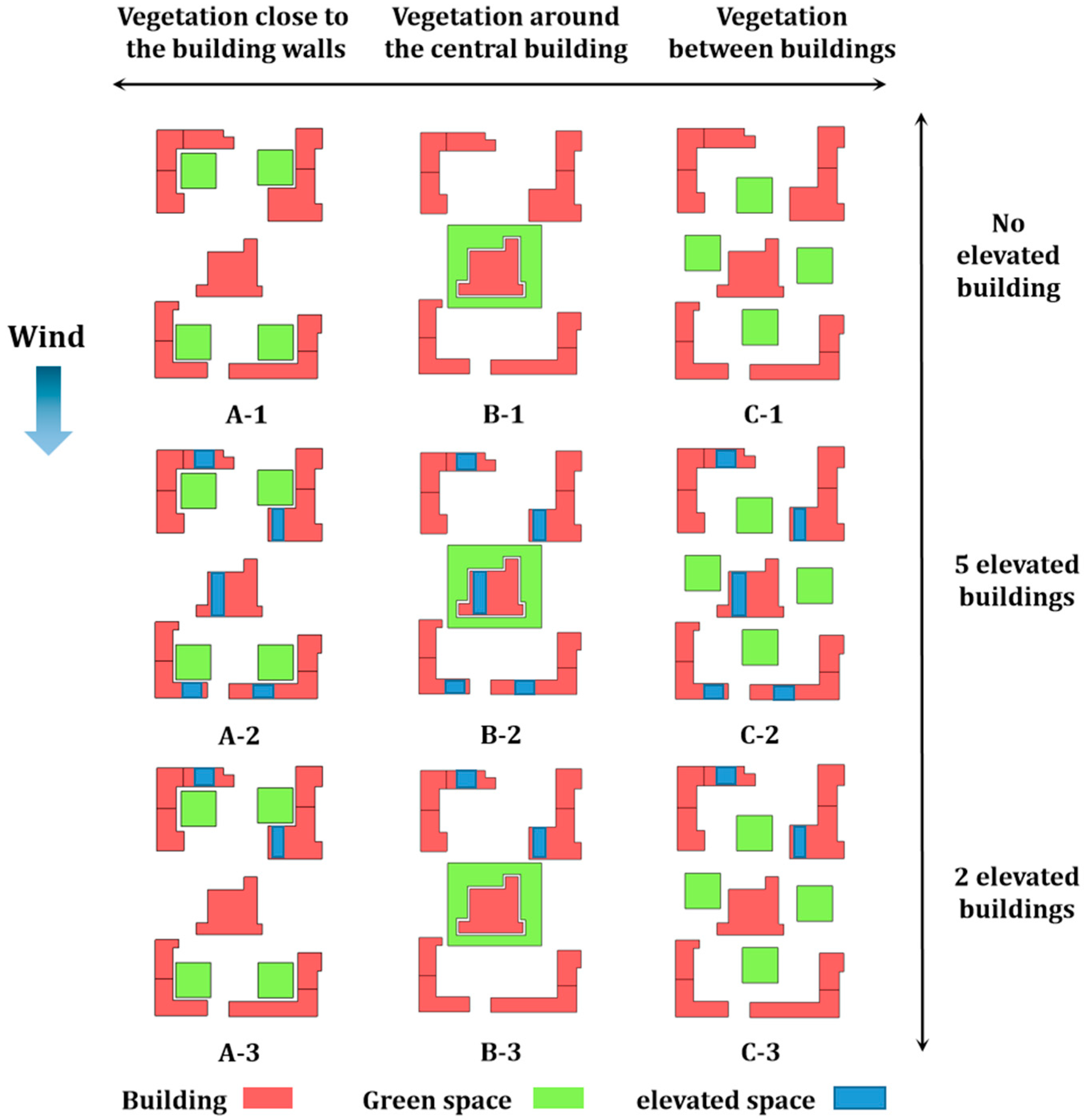
Based on the computational model, nine scenarios were established to explore how different layouts of vegetation and wind flow affected microclimate air temperatures. In the first step, three basic scenarios were created depending on different layouts of vegetation to solely analyze the effect of the vegetation layout, as follows:

• A-1: the vegetation was divided into four independent vegetation spaces with the same area for each, which were located close to the building walls.
• B-1: one unified vegetation space was located around the central building.
• C-1: four vegetation spaces that were the same size as in Scenario A were located between buildings.

In the second step, corresponding scenarios were set-up to examine the effect of wind flow in association with vegetation: three scenarios (A-2, B-2, and C-2) with five elevated spaces underneath all buildings were created to make extra wind paths through the buildings going north to south, and another three corresponding scenarios (A-3, B-3, and C-3) with two elevated spaces underneath the two northern buildings. All nine scenarios are shown in Figure 7.

Before simulating the nine scenarios, a case without vegetation and elevated space was explored. Figure 8 shows how wind flow occurred at 1.6 m height above ground; from the red part of the wind velocity contour, it can be seen that the high wind velocity appeared between buildings and around the central buildings by the Venturi effect, while wind velocity decreased as it got closer to the building walls. The air temperature for the vegetation-free scenario was 38.5 °C, and humidity remained the same as the initial weather conditions. Corresponding values of wind velocity, air temperature, and relative humidity reflected the area-weighted average results at the 1.6 m level within the boundary of the housing complex according to the CAD files.

3.1. Scenarios without an Elevated Space: A-1, B-1, C-1

Figure 9 shows how the wind velocity and air temperature at a 1.6 m height was different depending on three scenarios, A-1, B-1, and C-1, which had no elevated space. First, wind velocity was affected by the layout of vegetation. It was reduced to 1.08 m/s, 1.07 m/s, and 1.03 m/s in A-1, B-1, and C-1, respectively. It means that a vegetation space lowers wind flow and Scenario C-1 had the slowest wind velocity because vegetation spaces were located in the main wind path. Second, from the temperature contour in Figure 9, it is also observed how air temperature at a 1.6 m height was distributed by wind flow. In Scenario A-1, cooling air at vegetation spaces close to buildings remained in the study area, while it was dispersed outside the area by wind in B-1 and C-1. Especially, cooling air generated by the northern vegetation spaces in A-1 blocked hot air coming from the outside of the study area, while the hot air entered even inside the study area and was mixed with cooling air at the centered vegetation space, thereby diminishing the entire cooling performance in the study area.

As a result, A-1 was found to have the best cooling performance at a 1.9 °C reduction; the temperature was decreased to 36.6 °C at 1.6 m height from 38.5 °C when no vegetation. Therefore, it can be said that planning four independent vegetation spaces rather than one concentrated vegetation space is more efficient at reducing microclimate air temperature in the housing complex. Moreover, the effect of temperature reduction differs depending on how they are located; that is, it would be better to place small vegetation spaces close to a building rather than between buildings.

Regarding the humidity contour, it reflected the mass fraction of H₂O (vapor) in air. The transpiration process generated water vapor and ambient air temperature was decreased due to the latent heat. Similar distribution was observed between humidity and air temperature as they both were affected by the vegetation area.

3.2. Scenarios with Elevated Spaces: A-2, B-2, C-2 and A-3, B-3, C-3

Elevated spaces were modeled as an artificial wind path to examine the relationship between vegetation and wind flow in more detail. It is apparent that an elevated space worked as a wind path in that wind velocity was increased than scenarios without an elevated space. However, it was not true that the more wind paths, the better for air temperature reduction. Rather, Scenario A-3, B-3, and C-3, where two elevated spaces were installed only at the northern two buildings, showed better cooling performance for temperature reduction than scenarios of five elevated spaces.

As presented in Figure 10, the wind velocity of A-2, B-2, and C-2 with the five elevated spaces scenarios was 1.22 m/s, 1.11 m/s, and 1.10 m/s, respectively, which were faster than A-3, B-3, and C-3 with the two elevated spaces scenarios (1.09 m/s, 1.09 m/s, and 1.08 m/s, respectively). Yet, for the four independent green spaces, the air temperature of the five elevated spaces scenarios at a 1.6 m height were not lower than the two elevated spaces scenarios. As a result, the transpiration effect showed lower cooling ability when the five elevated spaces were installed for the four independent vegetation spaces. It can be explained by the air temperature contours that more cold air flew out through the southern elevated spaces in the five elevated spaces scenarios; thus, when the southern elevated spaces were removed in scenarios A-3 and C-3, the cold air generated by the vegetation could stay in the study area, thereby resulting in a better cooling performance than in the five elevated spaces scenarios.

Figure 11 shows the comparison of wind velocity and air temperature decrease at 1.6 m height by each scenario. In sum, Scenario A-1 was the most efficient design to reduce air temperature, while B-1, which had a centered vegetation area, was the opposite. There was a strong correlation between vegetation layout types, wind velocity, and air temperature. Figure 11 shows that wind velocity was the fastest in Scenario A-2 and the slowest in Scenario C-1. For the cooling performance, the results were the most optimal in order of Scenario A (A-1, A-2, and A-3), Scenario C (C-1, C-2, and C-3), and Scenario B (B-1, B-2, and B-3). This again indicated that Scenario A functions as the most efficient layout for the transpiration cooling effect, while Scenario B does the least inside the housing complex at a 1.6 m height. However, it implies that the wind velocity was not always correlated to air temperature in that it decreased in Scenario B-2, which showed the best cooling effect among the B scenarios.

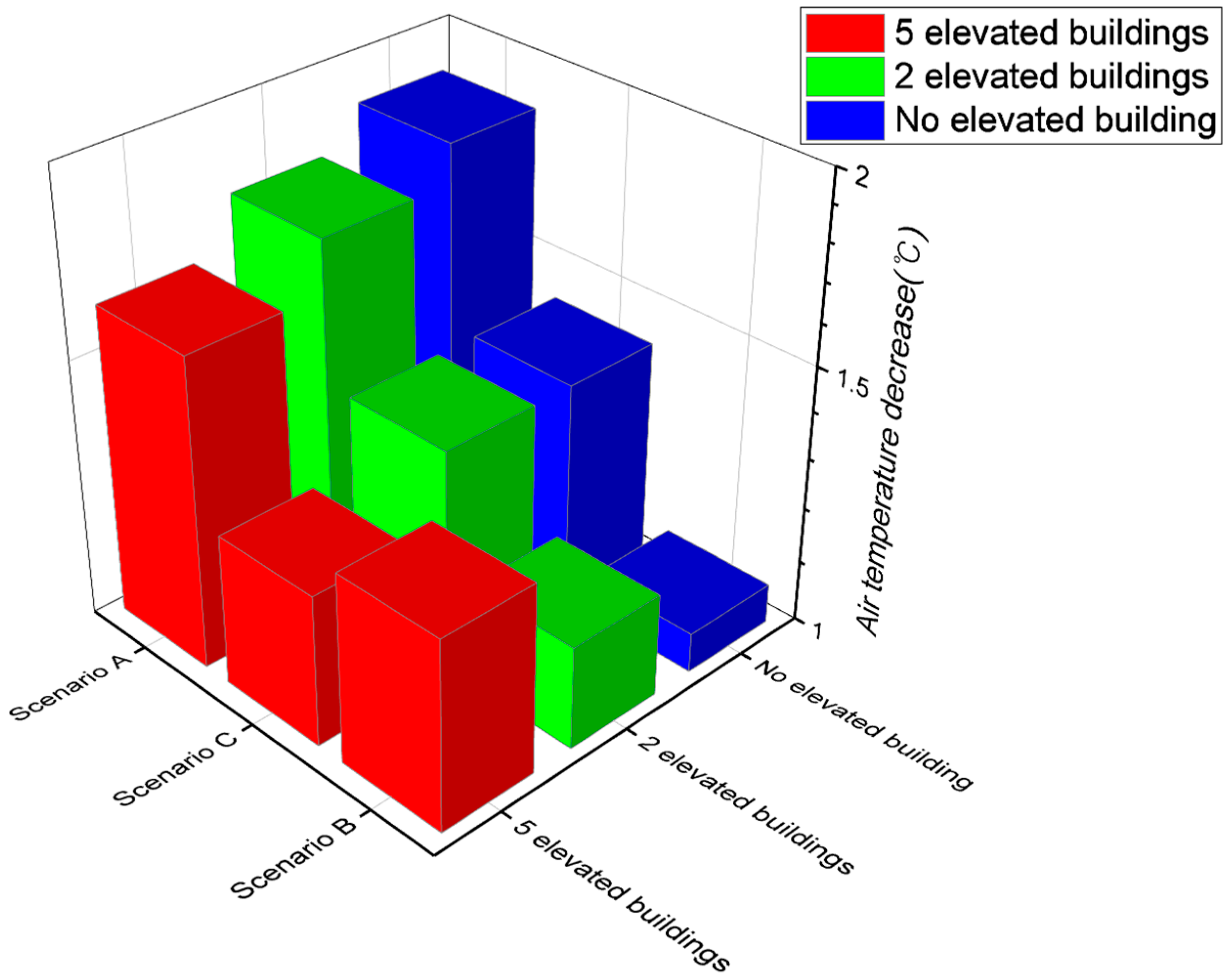
The comparison of air temperature decreased at the pedestrian level (1.6 m) depending on the vegetation scenarios and the number of elevated spaces, as is also shown in Figure 12. There was a clear trend in Scenario As and Scenario Cs that have four independent vegetation areas; the best cooling effect was found when no elevated space, followed by scenarios with two and five elevated spaces. In Scenario Bs with a centralized vegetation area, the outcome was opposite.

3.3. Temperature Change by Height

We also examined the air temperature decrease depending on height from 0 m to 30 m (

Table 2. Air temperature decrease between 0~30 m.

HEIGHT	A-1	A-2	A-3	B-1	B-2	B-3	C-1	C-2	C-3
0M	2.23	1.68	2.10	1.04	1.39	1.16	1.36	0.88	1.02
1.6M	1.87	1.63	1.76	1.06	1.35	1.18	1.42	1.27	1.42
5M	1.02	0.92	1.08	0.81	1.03	0.82	1.06	0.96	0.97
10M	0.49	0.46	0.52	0.47	0.50	0.52	0.48	0.47	0.53
15M	0.34	0.31	0.36	0.37	0.35	0.38	0.31	0.35	0.36
20M	0.29	0.27	0.34	0.30	0.31	0.31	0.24	0.31	0.33
25M	0.28	0.28	0.29	0.31	0.29	0.28	0.24	0.29	0.30
30M	0.26	0.26	0.27	0.29	0.26	0.27	0.23	0.28	0.25
AVERAGE	0.85	0.73	0.84	0.58	0.68	0.61	0.67	0.60	0.65

and Figure 13). From the data in Figure 13, the effect of temperature reduction by vegetation was clear for a 1.6 m height and below. Yet, above 10 m, only an approximately 0.5 °C was decreased in each scenario and the difference between scenarios was very small. This was an expected outcome because the cooling air was diluted in the upper region of the housing complex. Nevertheless, the results imply that different elevated space allocations affect the maximum transpiration cooling effect at different height levels. In Scenario A and C, A-1 and C-1, which had no elevated space, showed the best cooling performance between 0 m through 1.6 m, but, above 5 m, A-3 (5 m through 30 m) and C-3 (10 m through 25 m) with two elevated spaces showed the best. In Scenario B, B-2 with two elevated spaces showed the best cooling performance below 5 m, but B-3 between 10 m through 15 m did the best. It demonstrated that elevated spaces helped create a more cooling effect at higher regions, but weakened the effect below 5 m for the four independent vegetation scenarios (A and C). In B scenarios with one centralized vegetation area, however, the best cooling effect below a 1.6 m height was Scenario B-3 with the two elevated spaces installed. These results also led to a conclusion that the layout of vegetation should be carefully planned by considering wind flow to achieve more efficient cooling performance in the complex.

4. Discussion and Conclusions

The main aim of this study was to gain an understanding of the relationship of the outdoor cooling effect between vegetation and wind flow in an actual housing complex. To do this, we examined the difference of temperature reduction by spatial allocation of green spaces and wind flow through more elaborate CFD simulations under the actual built environment of an apartment housing complex in Seoul. It utilized ANSYS Fluent and built a real housing complex model with various possible scenarios, in which an approach integrated with a transpiration humidity effect was applied. Most of all, this study demonstrated that different layouts of vegetation and wind flow clearly affect microclimate air temperature in the housing complex. The entire analysis of our results has led to the following conclusions and implications.

First, vegetation reduced air temperature at a 1.6 m height by up to 1.9 °C in Scenario A-1 and at least 1.1 °C in Scenario B-1. It also works as a cool drainage, thereby reducing the microclimate air temperature of the surroundings. These results confirm previous studies regarding the vegetation’s cooling effect. Moreover, the amount of maximum temperature reduction was similar to the Gerogi et al.’s study [13], which demonstrated a 3.1 °C reduction through plant evapotranspiration. To identify a more accurate cooling effect for pedestrians, we introduced apparent temperature (AT), as it is easy to calculate and valid over a wide range of temperatures. It should be noted that, however, it is a simple bioclimatic index and there are some more sophisticated bioclimatic indices such as UTCI and PET [50,51]. Apparent temperature especially has different clothing thermal insulation assumptions compared to the advanced clothing model in UTCI, which is affected by relative humidity, wind speed, and air temperature [52].

$$AT=T_a+0.33\rho -0.7v-4.00$$

(6)

$$\rho =\frac{rh}{100}\cdot 6.105 {\exp }^{\left(17.27T_a/237.7+T_a\right)}$$

(7)

where AT is the apparent temperature in °C, T_a is the dry bulb temperature in °C; ρ is the water vapor pressure; v is the wind speed (m/s); and rh is the relative humidity.

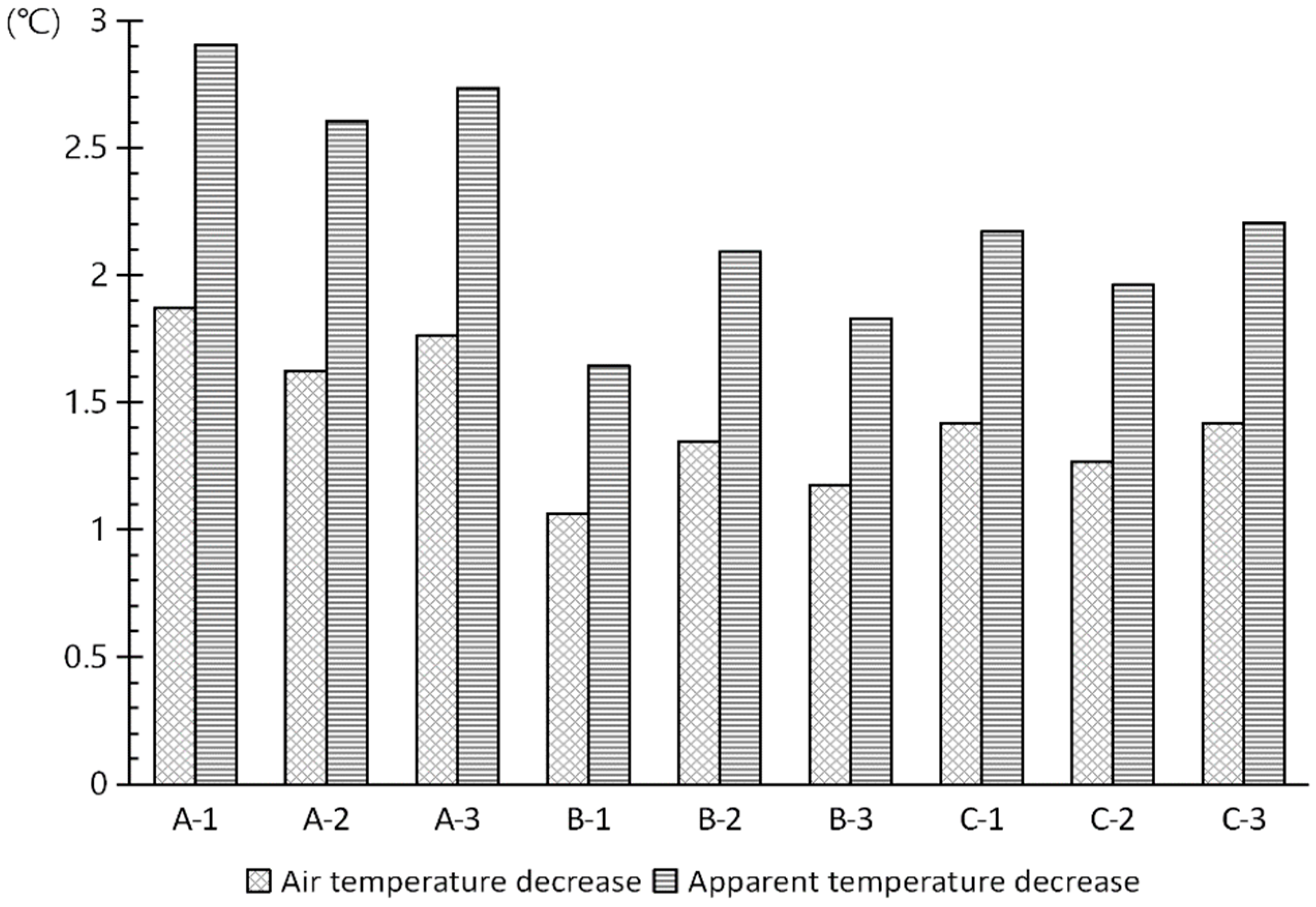
The apparent temperature calculated from the simulation results indicates that actual thermal comfort at the pedestrian level is more effective as shown in Figure 14. For example, in Scenario A-1 that showed the best cooling performance in all simulations, the actual effect of apparent temperature reduction for pedestrians reached 2.9 °C, which was 1.0 °C (55.3%) lower than the air temperature reduction in the simulation. In other scenarios, 0.8 °C (55.6%) on average was reduced. Therefore, it should be noted that the temperature reduction effect of vegetation is more effective for pedestrians than what was measured in simulations.

Second, when the total area of vegetation was the same, it was more effective to reduce air temperature by placing it in small units rather than concentrating it in one place; and placing small vegetation spaces close to buildings was better than locating them between buildings. This outcome can be explained by the effect of wind flow, as well as a site plan. Since cooling air is dispersed by wind flow, mitigating air temperature is related to how the vegetation spaces are placed considering the layout of buildings and wind flow. In Scenario A-1, the cooling air produced by northern vegetation spaces stayed inside the study area, while cooling air was more quickly dispersed by wind in Scenario B-1. In Scenario A-3, since the Venturi effect occurred between buildings and the vegetation spaces were located in the main wind path, ambient air cooled by vegetation spaces was quickly flown outside of the study area. Therefore, to mitigate microclimate temperatures in summer, the layout of buildings and wind flow should be concurrently considered when planning layouts of vegetation spaces.

Third, it was apparent that an elevated space worked as a wind path, leading to increasing wind velocity. However, it did not always positively affect hot temperatures. The most effective cooling performance, a 1.9 °C reduction at a 1.6 m height, was found in Scenario A-1, in which vegetation spaces were located close to buildings without an elevated space. Moreover, A-2, B-2 and C-2 that had five elevated spaces with four independent green spaces were not more effective in reducing air temperature than A-1, B-1 and C-1 as no elevated space scenarios. This was a different outcome from what we expected that an elevated space would help reduce air temperature because it would increase wind flow. It was also an opposite outcome from general findings in previous studies, which demonstrated that increasing wind flow or wind corridors positively mitigated air temperatures [5,16]. This may be explained by the increase in hot air flow inlets and more cold air flow out of the housing complex. Referring to Equation (2), it can be explained that the increase in the mass flow rate $\dot{m}$ can lead to a decrease in the temperature reduction $\Delta T$. It is worth mentioning that when the allocation was changed to a two elevated spaces scenarios, the cooling performances of A-3 and C-3 obtained results closer to those of Scenario A-1 and C-1. On the other hand, for Scenario B (with a centralized vegetation area), it provided more air temperature decreases when there were increasing elevated spaces. Thus, it can be said that increasing airflow is likely to bring better outdoor thermal mitigation only for centralized vegetation in the housing complex.

It seems that the wind flow through elevated spaces located at the northern buildings brought hotter air outside of the study area into the courtyard, which negatively affected the overall cooling performance. To examine this hypothesis, we performed an extra simulation. In the simulation, the height of the northern building was raised to the same height as the other part of the building (Figure 15) under Scenario A, which showed the best cooling effect.

As shown in Figure 16, the scenarios with a higher northern wall produced a positive influence on average temperature reduction at a 1.6 m height. It explains how inlet hot air affects average temperature inside. Sectional diagrams in Figure 16 shows how wind flow blows out cold air through elevated spaces. Nevertheless, the original result that Scenario A-1, which had no elevated space, had better cooling performance than Scenario A-2 with five elevated spaces and Scenario A-3 with two elevated spaces was not changed.

Therefore, to mitigate air temperature at the microclimate level, a vegetation space and an elevated space should be designed by considering not only the direction of wind flow, but also the physical conditions inside and outside a housing complex.

This study aimed to understand how different layouts of vegetation and wind flow affect microclimate air temperatures by the cooling performance of vegetation via ANSYS Fluent, which is a more precise simulation tool. Nevertheless, this study had some limitations. The RANS models, which can meet the demands of common engineering simulations, are widely used and validated; but, LES and DES that depict turbulence in detailed information are more elaborate than RANS models. In addition, since this study simulated one housing complex in Seoul, which has a courtyard surrounded by buildings, more simulations with different types of housing complex are required to gain a general conclusion on the relationship between spatial allocation of vegetation and cooling effect in an association with wind flow. A future study is also necessary to validate the vegetation model that includes the humidity effect of transpiration. Plus, comprehensive bioclimatic indices such as PET or UTCI would be useful to investigate the effect of surface infrared radiation (IR) in a future study.