Land Use and Land Cover Scenarios for Optimum Water Yield and Sediment Retention Ecosystem Services in Klong U-Tapao Watershed, Songkhla, Thailand

Abstract

The Klong U-Tapao watershed is the main source of water supply for agriculture, industry, and household consumption of the Songkhla province and it frequently contributes serious problems to lowland areas, particularly flood and soil erosion. Therefore, land use and land cover (LULC) scenario identification for optimum water yield and sediment retention ecosystem services are necessary. In this study, LULC data in 2010 and 2017 were firstly classified from Landsat data using random forests classifiers, and they were then used to predict LULC change during 2018 –2024 under three different scenarios by CLUE-S model. Later, actual LULC data in 2017 and predictive LULC data of three scenarios were further used to estimate water yield and sediment retention services under the InVEST and LULC scenario for optimum water yield and sediment retention ecosystem services were finally identified using the ecosystem service change index (ESCI). The result of the study showed the major increasing areas of LULC types during 2010–2017 were rubber plantation and urban and built-up area while the major decreasing areas of LULC classes were evergreen forest and miscellaneous land. In addition, the derived LULC prediction of three different scenarios could provide realistic results as expected. Likewise, water yield and sediment retention estimation of three different scenarios could also provide expected results according to characteristics of scenarios’ definitions and climates, soil and terrain, and LULC factors. Finally, LULC of Scenario II was chosen for optimum water yield and sediment retention ecosystem services. In conclusion, the integration of remote sensing technology with advanced classification methods and geospatial models can be used as proficient tools to provide geospatial data on water yield and sediment retention ecosystem services from different scenarios.

1. Introduction

Water yield is the sum of runoff from the landscape [1,2]. The relative water volume in a given landscape affects the quality of ecology in the area [3]. Therefore, changes in the landscape that affect the annual average water yield can increase or decrease land productivity. For example, replacing forests on slope land or mountainous areas with rubber plantations results in water retention in the subsoil layer and decreases water discharge in the dry season and increases evapotranspiration [4]. In contrast, cultivated land leads to larger average amounts of surface runoff and higher water loss from the reduced evapotranspiration in the wet season. The increase in water yield may cause floods and landslides. The water yield is reflected as cumulative surface runoff measured at a specific location; therefore, it is not the desired type of regulation of water flow with yield and quality. However, high water yield is an ecosystem service, as is surface runoff, which is dependent on the vegetation cover under a given land use; thus, over-surface runoff is not an appropriate situation as an ecosystem service [5,6].

The processes of soil erosion, sediment retention, and sediment transport are key components and functions of the watershed area [7,8,9,10]. Increases in sediment yield are manifested worldwide, affecting water quality, reservoir management, and natural water resources [11,12]. The sediment retention service provides by natural landscapes is of great interest to water managers [13]. Understanding where the sediments are produced and delivered allows managers to design improved strategies for reducing sediment loads [14,15]. Changes in sediment load can have negative impacts on downstream irrigation, water treatment, recreation, and reservoir performance [14,16]. Erosion and overland sediment retention are foundations for ecosystem management that govern the sediment concentration in streams [17]. Sediment dynamics at the watershed scale are mainly controlled by climate, in particular, the rain intensity, soil properties, topography, and vegetation and conservation practice [18,19,20]. The cause of soil erosion resulting from the deterioration of a watershed shows as greater sediment deposits [21]. The soil erosion rates with land use and land cover (LULC) changes indicated that cleared land in a watershed will generate the highest soil losses. The vegetation cover protects the soil from the direct impact of raindrops or heavy rain, which invariably reduces soil loss to the bare land [22].

Data from the optical satellite sensor of Landsat data have been used to LULC map and to assess ecological variables in Southeast Asia [23,24,25,26]. Landsat TM and OLI, random forest machine learning algorithms, can achieve accurate LULC map classification with high overall accuracy and the Kappa hat coefficient [27,28]. The CLUE-S model has been used to simulate the spatial dynamics and spatial allocation of land use types under different scenarios in Thailand [29,30,31]. The model treats the competition between different types of land uses for land allocation based on logistic model analysis [32].

The multiple ecosystem service evaluations are estimated using the variety toolsets of the InVEST software suite for assessing the impact of land use scenarios at the watershed level. The Water Yield model of the InVEST has been applied to simulate the annual biophysical contribution of LULC to water yield [33]. It is flexible for use at the local or regional scale and the results about water yield, water consumption, and water supply mapping can be applied for decision making support [34]. The Sediment Delivery Ratio (SDR) model has been applied by many researchers to assess soil erosion, sediment retention and sediment export [34]. Lastly, the ecosystem service change index (ESCI) is used to calculate the change (gain and loss) of each ecosystem service and these are then integrated to provide an overall assessment of ecosystem services status for a location [35]. This provides the critical information needed in the design of management strategies for the ecosystem services.

The problems related to the Khlong U-Tapao watershed under the Songkhla Lake Basin (SLB) include a broad range of water resource development and land management, particularly flood and soil erosion. Water shortage is a problem in the dry season, impacting mainly the water supply for the industrial and agricultural sectors. Additionally, population growth also effectuates LULC change and agricultural land expansion, as an implication of meeting people’s economic needs, which might potentially produce water yield and erosion increase [29,30,36].

Flooding in lowland areas of the Klong U-Tapao watershed at Hat Yai city, Songkhla province also poses regular problems and heavy rainstorms occur every 2 or 3 years, causing inundation of the area. In addition, the high water level in the Gulf of Thailand usually mains to drainage problems in the rainy season. In the meantime, soil erosion is another principal issue associated with unsuitable land management, the cultivation of rubber and other crops on steep hills cause erosion. Deforestation generally results in the land being abandoned, and the cleared land rapidly erodes. In fact, rubber plantations have encroached into many places of the SLB, including Kao Pu Kao Ya National Park. Currently, 30 percent (144 km²) of the protected forest land (Watershed Class I) of the Khlong U-Tapao watershed under the SLB has been converted to rubber plantations [37]. These activities have increased soil erosion and sedimentation in Songkhla Lake [38]. Many factors drive on soil erosion in the Khlong U-Tapao watershed include unsuitable practices for rubber plantation and palm oil and deforestation [39]. So, the mitigation of flooding by reducing runoff and prevention of soil erosion by increasing sediment retention is considered as an important regulated ecosystem service in the study area. The aim of the research is to identify the scenario of LULC for optimum water yield and sediment retention ecosystem services in the Klong U-Tapao watershed, Songkhla Province, Thailand. The specific objectives of the study were (1) to classify LULC status and its change from 2010–2017, (2) to predict LULC change of three different scenarios (Scenario I: Trend LULC; Scenario II: Forest conservation and prevention; and Scenario III: Agriculture production) between 2018 and 2024, (3) to assess water yield and sediment retention, and (4) to identify LULC scenario for optimum water yield and sediment retention ecosystem services.

2. Materials and Methods

2.1. Study Area

The study area is the Khlong U-Tapao watershed under the SLB consists of 10 sub-watersheds: Khlong Bang Klam, Khong Wa, Khong Wat/Khong Tam, Khong Pom, Khong La/Khong Jam Rai, Khong Tong/Khong Pra Tu, Khong Ram, Khong Phang La/Khong Ngae, Khong Lea and Khong Sa Dao. It covers area of 2406.04 km² with 60 km length and 40 km width (Figure 1).

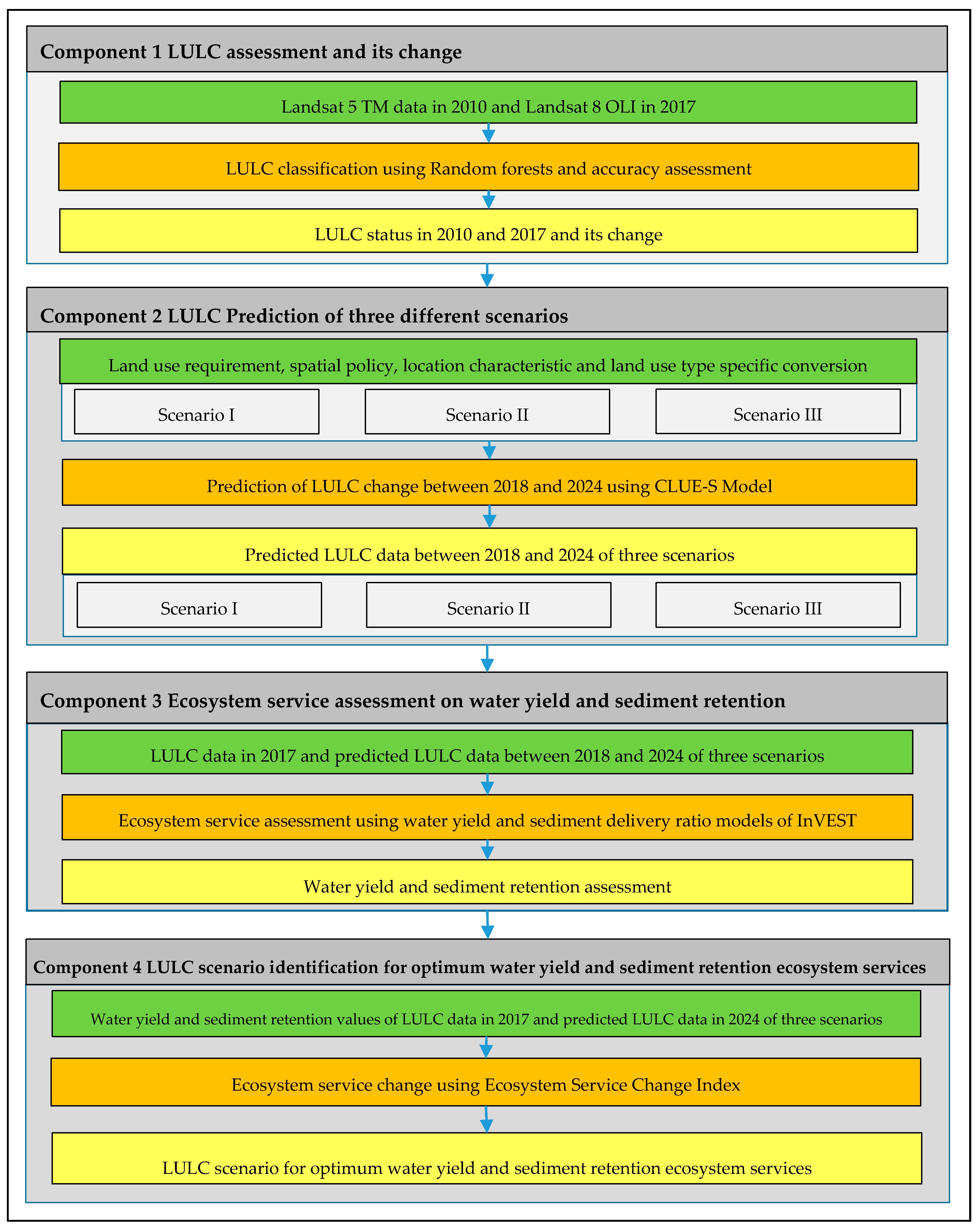
2.2. Research Methodology

The research methodology workflow (input, process, and output) consisted of 4 components: (1) LULC assessment and its change; (2) LULC prediction of three different scenarios; (3) ecosystem service assessment on water yield and sediment retention; and (4) LULC scenario identification for optimum water yield and sediment retention ecosystem service (Figure 2). Details of each component were described in the following sections.

2.2.1. LULC Assessment and Its Change

For this component, two standard product of scaled reflectance data at Level 2 of Landsat 5-TM dated 7 May 2010 (band 1, 2, 3, 4, 5, and 7) and Landsat 8-OLI dated 23 March 2017 (band 2, 3, 4, 5, 6, and 7) were downloaded from USGS website (www.earthexplore.usgs.gov) for LULC classification using the RF. In practice, homogeneous training areas of each LULC type including (1) urban and built-up area, (2) paddy field, (3) rubber plantation, (4) oil palm plantation, (5) perennial tree and orchard, (6) aquatic culture area, (7) evergreen forest, (8) mangrove forest, (9) marsh and swamp, (10) water body, and (11) miscellaneous land (bare land and abandoned mine) were separately prepared to extract multiple decision trees for LULC classification by the EnMap-Box software [40]. In principle, the predicted LULC type of observation is calculated based on the majority vote of the trees under the RF model, and the discrimination function is defined using Equation (1) [41].

$$H\left(x\right)=argma{x}_y{\displaystyle {\displaystyle \sum }_{i=1}^k}I(h_i(X,{\theta }_k)=Y)$$

(1)

where $I$ is the indicator function, $h_i\left(X,{\theta }_k\right)$ is single decision tree, and $Y$ is the output variable, $argma{x}_y$ denotes the $Y$ value when maximizing ${{\displaystyle \sum }}_{i=1}^{k}I(h_i(X,{\theta }_k)$.

Then, the preliminary LULC maps in 2010 and 2017 were assessed accuracy (overall accuracy, producer’s accuracy, user’s accuracy and Kappa hat coefficient) based on the reference data from Google Image in 2010 and field survey in 2017, respectively. Herein, the number of sample sizes for thematic accuracy assessment was estimated based on multivariate statistics with stratified random sampling scheme as suggested by Congalton and Green [42]. In this study, the number of sample points for accuracy assessment was 880 points, with the desired precision of 95%. Lastly, final LULC maps in 2010 and 2017 were further used to detect LULC change using post-classification comparison algorithm. The derived results (LULC in 2010 and 2017) were further applied for LULC prediction between 2018 and 2024 in three different scenarios using the CLUE-S model.

2.2.2. LULC Prediction of Three Different Scenarios

This study used the CLUE-S (Conversion of Land Use and its Effects at Small regional extent) model to predict LULC between 2018 and 2024 in three different scenarios. The CLUE-S model is based upon an analysis of location suitability using logistic regressions and simulates the competition and interactions between the different LULC types. The basic concept and its development of this model was explained in more detail by [43,44].

Under the CLUE-S model, logistic regression analysis (Equation (2)) was performed to identify LULC type location preference according to driving force on LULC change after multicollinearity test. In this study, 8 driving factors on LULC change include elevation, slope, soil fertility, distance to road, distance to settlement, distance to water bodies, population density at sub-district level and average household income at sub-district level were examined as same as Reference [31]. Based on group discussion (participatory method) among stakeholders inside and surrounding the watershed including local people, NGOs and government agencies (Provincial Agriculture Office, Regional Office of Agricultural Economics, Regional Irrigation Office, Protected Areas Regional Office, Forest Resource Management Office, Prince of Songkhla University and Thaksin University), three future LULC scenarios were proposed including:

Scenario I: Trend LULC. The prediction of LULC in 2024 relies on the historical trend of LULC change between 2010 and 2017. Herein, land requirement (demand) for LULC prediction during 2018–2024 is based on the annual change rate of LULC between 2010 and 2017 from the transition area matrix using the Markov Chain model.

Scenario II: Forest conservation and prevention. Under this scenario, the existing government policy on forest conservation and prevention is integrated and transformed into forest land demand. Herein, the legal boundary of the national park, wildlife sanctuary, watershed class IA and an existing forest area in 2017 is used as forest land demand for LULC prediction in the same period.

Scenario III: Agriculture production extension. Under this scenario, government policy on agricultural production extension by zonation in the future was reviewed and transformed into land demand for optimum land utilization for oil palm plantation based on suitability map of Department of Agriculture in 2015. Additionally, the existing forest area (evergreen and mangrove forests) in 2017 is preserved under LULC prediction during 2018–2024. The quantitative information of land requirement in 2024 of three different scenarios according to their definitions is summarized in

Table 1. The land requirement of three different scenarios in 2024.

LULC Type	Base Line Data in 2017 (Km2)	Land Requirement in 2024 (Km2)
		Scenario I	Scenario II	Scenario III
Urban and built-up area	113.21	145.4 1	145.4 1	145.41 1
Paddy field	20.41	14.59 1	20.4 2	20.41 2
Rubber plantation	1,727.46	1,736.85 1	1,568.17 3	1,524.88 4
Oil palm plantation	18.85	32.35 1	32.35 1	259.51 5
Perennial tree/orchard	34.20	37.05 1	34.20 2	34.20 2
Aquatic cultural area	9.38	10.18 1	9.38 2	9.38 2
Evergreen forest	254.01	202.57 1	377.47 6	254.01 2
Mangrove forest	0.85	0.93 1	0.85 2	0.85 2
Marsh and swamp	42.70	37.50 1	42.70 2	37.50 1
Water body	42.43	50.93 1	42.43 2	42.43 2
Miscellaneous land	142.57	137.72 1	132.69 7	77.49 8

Note: ^1. Land requirement of a specific LULC type was based on annual change rate of each LULC between 2010 and 2017 from transition area matrix by Markov Chain model; ^2. Land requirement of a specific LULC type was fixed based on its area in 2017; ^3. Land requirement of rubber plantation was decreased since an illegal rubber plantation in the protected area (national park, wildlife sanctuary, watershed class IA) will be revoked and replaced by forest plantation; ^4. Land requirement of rubber plantation was decreased since rubber plantation that situates in oil palm suitability zones will be replaced by new oil palm plantation; ^5. Land requirement of oil palm plantation was increased according to the strategic plan to expand oil palm plantation. Herein, rubber plantation and miscellaneous land in 2017 that situate in suitable zones for oil palm plantation will be replaced by new oil palm plantation; ^6. Land requirement of evergreen forest was increased according to reclamation forest areas back from intruders under reforestation program in an illegal rubber plantation and miscellaneous land that situate in the protected forest area (national park, wildlife sanctuary, watershed class IA); ^7. Land requirement of miscellaneous land was decreased since it will be replaced by forest plantation; ^8. Land requirement of miscellaneous land in 2024 was decreased since it will be replaced by new oil palm plantation.

.

$$Log\left(\frac{P_i}{1-P_i}\right)={\beta }_0+{\beta }_1{X}_{1,i}+{\beta }_2{X}_{2,i}\dots +{\beta }_n{X}_{n,i}$$

(2)

where, P_i is the probability of a grid cell for the occurrence of the considered land use type on location i and the X’s are the location factors. The coefficients (β) are estimated through logistic regression using the actual land use pattern as the dependent variable [32].

2.2.3. Ecosystem Service Assessment on Water Yield and Sediment Retention

Water Yield Estimation

To estimate water yield from the Water Yield model of InVEST, annual water yield, Y(x) for each pixel on the landscape (x) was calculated [45] as:

$$Y\left(x\right)=\left(1-\frac{AET\left(x\right)}{P\left(x\right)}\right)·P\left(x\right)$$

(3)

where, AET _(x) is the annual actual evapotranspiration on each pixel x and P_(x) is the annual precipitation on each pixel.

In practice, relevant factors of Water Yield model were prepared in advance as followings (see in Appendix

Table A1. Minimal root depth and plant evapotranspiration coefficient for each LULC type.

LULC Type	Root Depth (mm)	Kc	References
Urban and built-up area	0	0.3	[45,80]
Paddy field	400	0.6	[81]
Rubber plantation	2500	0.9	[45,80]
Oil palm plantation	2000	0.9	[45,80]
Perennial tree and orchard	3000	0.95	[45,80]
Aquatic cultural area	0	0	[45,80]
Evergreen forest	7300	1	[45,80]
Mangrove forest	500	1	[45,80]
Marsh and swamp	200	0.7	[82]
Water body	0	0	[45,80]
Miscellaneous land	0	0	[45,80]

).

(1) Annual rainfall. Available annual rainfall records of TMD (Thai Meteorological Department) between 2010 and 2017 were collected from Reference [46] to calculate water yield for validation. Meanwhile, annual rainfall data between 2018 and 2024 were downloaded from the Global Products and Data Services of the National Center for Atmospheric Research [47] for water yield estimation. In this research, the simulated rainfall data between 2018 and 2024 under RCP_8.5 scenario, which represents the highest rising of radiative forcing pathway (8.5 W/m²), population probability, economic trends, greenhouse gas emission level, and technological change [48], were selected to characterize the impact of climate change on water yield.

(2) Root restricting layer depth. Soil depth under soil series data of Reference [49] was applied to generate the root-restricting layer depth for water yield estimation.

(3) Plant available water content (PAWC). The PAWC is defined as the difference between the fraction of volumetric field capacity and permanent wilting point, which is an important influencing factor of crop production, agro-ecological zoning, irrigation planning, and land cover changes. The PAWC was estimated based on the relationship between PAWC and the physical and chemical properties of soil (sand, silt, clay and organic matter) [50] as:

PAWC = 54.509 − 0.132 × sand% − 0.003 × (sand%) ² − 0.055 × silt% − 0.006 × (silt%) ²
−0.738 × clay% + 0.007 × (clay%) ² − 2.688 × OM% + 0.501 × (OM%) ²

(4)

where, PAWC is the plant available water fraction (%) represent the measured contents of sand (%), clay (%), silt (%) and organic matter (%).

(4) Annual potential evapotranspiration (PET). Annual PET is estimated using the modified Hargreaves’ equation as suggested by Reference [51] as:

$$PE{T}_0=0.0013\times 0.408\times RA\times \left(T_{avg}+17\right)\times {(TD-0.0123P)}^{0.76}$$

(5)

In principle, the modified Hargreaves uses the average of the mean daily maximum and mean daily minimum temperatures (T_avg in °C), the difference between mean daily maximum and mean daily minimums (TD), extraterrestrial radiation (RA) in MJm⁻²d⁻¹ and precipitation (P) in mm per month. Herein, temperature and precipitation data in 2017 and 2024 were extracted and predicted from meteorological stations of Reference [46] while radiation data is generated by solar radiation tool within the ESRI ArcGIS software. Then, the PET₀ equation was calculated by Model Builder within the ESRI ArcGIS software again.

(5) Biophysical factor. A biophysical factor table contains LULC code, descriptive name of LULC, the maximum root depth for vegetated land use classes in millimeters and the plant evapotranspiration coefficient for each LULC type. Herein, the evapotranspiration coefficient (Kc) of each land use type was gathered from the previous studies in Thailand as shown in Appendix Table A1.

Sediment Retention Estimation

Sediment retention was estimated using multiplication operation between soil erosion and sediment delivery ratio under the SDR model of InVEST. In practice, amount of annual soil loss on pixel i, A_i was estimated using the Revised Universal Soil Loss Equation (RUSLE) by Renard and Freimund [52] as:

$$A_i=R_i·K_i·{LS}_i{C}_i·P_i$$

(6)

where A_i is annual soil erosion (ton. ha⁻¹ yr⁻¹), R_i is rainfall erosivity (MJ mm ha⁻¹ h⁻¹ y⁻¹),

K_i is soil erodibility (ton⋅ha⋅hr (MJ⋅ha⋅mm)⁻¹), LS_i is slope length-gradient factor,

C_i is crop-management factor, and P_i is support practice factor for erosion control.

Brief information of relevant factors for soil erosion estimation are summarized below.

(1) Rainfall erosivity (R). The rainfall erosivity factor was calculated as suggested by Reference [53] and modified by Reference [54]. Rainfall data in 2017 collected from the TMD [46] was used for calculating R-factor in RUSLE by Equation (7).

$$R={\displaystyle {\displaystyle \sum }_{i=1}^{12}}1.735\times {10}^{\left(1.5lo{g}_{10}\left(\frac{P_i^2}{P}\right)-0.08188\right)}$$

(7)

where $R$ is the rainfall erosivity factor (MJ mm ha⁻¹ h⁻¹ y⁻¹), $P_i$ is the monthly rainfall (mm), and $P$ is the annual rainfall (mm).

(2) Slope length gradient factor (LS). The LS factor was calculated from the Digital Elevation Model (DEM).

(3) Soil erodibility (K). The K-factor was adopted from standard values of Reference [55], which are extracted from soil series data (see in Appendix

Table A2. Soil series and soil erodibility factor values [55].

Soil Series	Erodibility Factor Value	Soil Series	Erodibility Factor Value
Ban Thon series	0.20	Rangae/Tha Chin association	0.14
Bang Klam series	0.12	Rangae series	0.20
Bang Nara/Kokiean association	0.30	Ranong/Hat Yai association	0.32
Bang Nara series	0.26	Ranong/Phato association	0.25
Chumphon/Sawi association	0.28	Ranong series	0.23
Chumphon series	0.28	Ranote series	0.14
Complex of well drained, levee soil	0.22	Rayong series	0.23
Hat Yai/Padang Baser association	0.27	Residential	0.11
Hat Yai series	0.27	Ruso series	0.22
Khlong Nok Kra Thung series	0.20	Sai Buri fine clayey variant	0.26
Khlong Thom series	0.25	Sai Buri, fine clayey variant/Ruso association	0.28
Kho Hong/Tha Sae, mottled variant association	0.27	Sai Kao, somewhat excessively drianed variant	0.25
Kho Hong series	0.24	Samut Prakan series	0.17
Khok Khian fine sand fraction variant	0.17	Sathon series	0.28
Khok Khian series	0.24	Sawi series	0.20
Klaeng series	0.27	Slope Complex	0.21
La Harn series	0.22	Songkla Lake	0.07
Lang Suan series	0.13	Swamp	0.24
Nam Krachai/Kho Hong association	0.23	Tha Sae, mottled variant	0.25
Nam Krachai series	0.23	Tha Sae, mottled variant/Klaeng association	0.27
Padang Besar series	0.28	Thung Wa series	0.21
Pawong/Rangae association	0.23	Tin mine land	0.20
Pawong series	0.14	Visai complex	0.29
Phato series	0.22	Visai series	0.24
Puket series	0.20	Yala series	0.27

)

(4) Cover factor (C). LULC data in 2010 and 2024 from three scenarios were used as input data to extract C factor value based on the standard assignment of Reference [55] (see in Appendix

Table A3. C and P factor corresponding to each LULC class [55].

LULC Type	C Factor	P Factor
Urban and built-up area	0	0
Paddy field	0.4	1
Rubber plantation	0.22	1
Oil palm plantation	0.3	1
Perennial tree and orchard	0.3	1
Aquatic culture area	0	0
Evergreen forest	0.001	1
Mangrove forest	0	0
Marsh and swamp	0.40	1
Water body	0	0
Miscellaneous land	0.6	1

).

(5) Practice factor (P). P factor values were extracted from LULC data based on the standard assignment of Reference [55] (see in Appendix Table A3).

Then, soil delivery ratio (SDR) was secondly estimated using connectivity index (CI) that reflecting the attributes of each LULC type, threshold flow accumulation and maximum SDR. The SDR value was calculated as suggested by [56] as:

$$SD{R}_i=\frac{SD{R}_{max}}{1+exp\left(\frac{I{C}_0-I{C}_i}{k}\right)}$$

(8)

where, SDR_max is the maximum theoretical SDR, set to an average value of 0.8 [57], and IC₀ and k are calibration parameters that define the shape of the SDR-IC relationship (increasing function).

Finally, sediment retention was estimated as suggested by Reference [45] as:

$$Sedimentretention=R\times K\times LS\left(1-CP\right)\times SDR$$

(9)

Moreover, the existing water yield (runoff) and sediment export data between 2010 and 2017 at X.90 station of the Royal Irrigation Department [58] were used to validate water yield (runoff) and sediment delivery ratio model using NSE (Nash-Sutcliffe Efficiency) and Coefficient of determination (R²).

2.2.4. LULC Scenario Identification for Optimum Water Yield and Sediment Retention

The analyzed ecosystem services change the state of water yield and sediment retention due to LULC change was assessed using ESCI as suggested by [35] as:

$${ESCI}_X=\left[\frac{E{S}_{CUR{x}_j}-E{S}_{HIS{x}_i}}{E{S}_{HIS{x}_i}}\right]$$

(10)

where, ESCIx is the ecosystems services change index of service X, $E{S}_{CUR{x}_j}$ and $E{S}_{HIS{x}_i}$ are the current and historic ecosystem service state values of service X at times j and i, respectively.

In this study, historical ecosystem service values (water yield and sediment retention) was based on LULC in 2017 while the current ecosystem service was based on the predicted LULC between 2018 and 2024. To extract gain and loss of ecosystem services (water yield and sediment retention), historical ecosystem service values in 2017 and annual ecosystem services values between 2018 and 2024 were separately calculated pair by pair using Equation (10). The derived results were then averaged to identify LULC scenario for optimum water yield and sediment retention ecosystem services.

3. Results

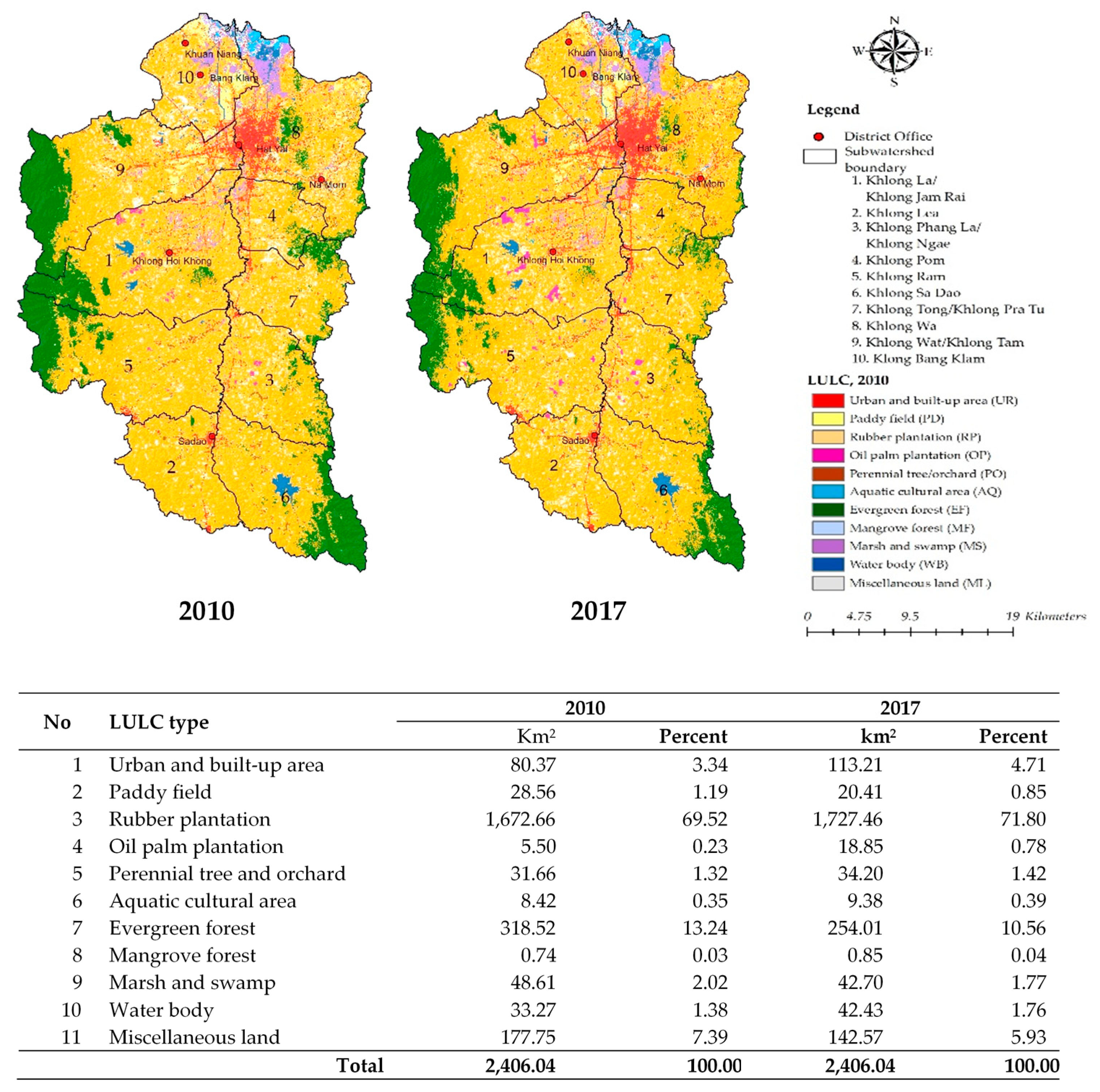
3.1. LULC Assessment and Its Change

Rubber plantations, urban and built-up area substantially increased from 2010–2017. In fact, rubber plantation covered area of 1,672.66 km² or 69.52% in 2010 and 1727.46 km² or 71.80% in 2017. Likewise, urban and built-up area in this period were 80.37 km² or 3.34% and 113.21 km² or 4.71% respectively. On the contrary, evergreen forest and miscellaneous land use decreased rapidly in the same period. Evergreen forest and miscellaneous land covered area of 318.52 km² or 13.24% and 177.75 km² or 7.39% in 2010 and covered area of 254.01 km² or 10.56% and 142.57 km² or 5.93% in 2017 (Figure 3). In addition, the derived overall accuracy and Kappa hat coefficient for classified thematic LULC map in 2010 and 2017 were 91.36% and 84.00%, and 94.32% and 87.00%, respectively.

The transitional change matrix of LULC between 2010 and 2017 (

Table 2. LULC change between 2010 and 2017 as a transitional matrix.

	LULC Types	LULC 2017 (km2)
		UR	PD	RP	OP	PO	AQ	EF	MF	MS	WA	ML	Total
LULC2 010 (km2)	Urban and built-up area (UR)	80.37	-	-	-	-	-	-	-	-	-	-	80.37
	Paddy field (PD)	0.61	20.41	6.55	0.02	0.08	-	-	-	-	0.20	0.70	28.56
	Rubber plantation (RP)	24.52	-	1528.37	12.06	-	-	-	-	-	6.78	100.93	1672.66
	Oil palm plantation (OP)	-	-	-	5.50	-	-	-	-	-	-	-	5.50
	Perennial tree/orchard (PO)	0.67	-	-	-	30.43	-	-	-	-	-	0.57	31.66
	Aquatic cultural area (AQ)	-	-	-	-	-	8.42	-	-	-	-	-	8.42
	Evergreen forest (EF)	0.05	-	63.33	0.14	0.30	-	254.01	-	-	0.20	0.49	318.52
	Mangrove forest (MF)	-	-	-	0.01	-	0.02	-	0.64	-	0.02	0.06	0.74
	Marsh and swamp (MS)	0.93	-	-	0.28	0.16	0.40	-	0.22	42.70	1.37	2.56	48.61
	Water body (WA)	-	-	-	-	-	-	-	-	-	32.21	1.06	33.27
	Miscellaneous land (ML)	6.07	-	129.21	0.85	3.24	0.54	-	-	-	1.64	36.22	177.75
	Total	113.21	20.41	1727.46	18.85	34.20	9.38	254.01	0.85	42.70	42.43	142.57	2406.04

) indicated that approximately 24.52 km² of rubber plantations were converted to urban and built-up areas during this period and followed by miscellaneous land 6.07 km². Meanwhile, approximately 12.06 km² of rubber plantations were transformed to oil palm plantation as the result of government policy (Ministry of Agriculture and Cooperatives, 2014). Nevertheless, about 73% of miscellaneous land (129.21 km²) and 20% of evergreen forests in 2010 (63.33 km²) were converted into rubber plantations.

3.2. LULC Prediction of Three Different Scenarios

The result of multicollinearity test among independent variables (driving force on LULC change) with VIF values is summarized in

Table 3. Multicollinearity statistics test of driving factors effect to LULC type.

Independent Variable (Driving Force on LULC Change)	Unstandardized Coefficients		Standardized Coefficient	VIF
	Beta	Std. Error
Elevation	0.0054	0.0001	0.2743	3.6138
Slope	0.0017	0.0004	0.0094	1.3602
Distance to water bodies	−0.0001	0.0000	−0.0681	1.4320
Distance to road	0.0000	0.0000	0.0129	4.1062
Distance to settlement	0.0001	0.0000	0.0904	5.1322
Soil fertility	0.1152	0.0065	0.0358	1.1509
Population density at sub-district level	−0.0003	0.0000	−0.0768	1.0649
Average household income at sub-district level	0.0000	0.0000	0.0077	1.1218

. It indicated that none of the variables have highly correlated with each other since all independent variables have VIF < 10 [59,60].

Meanwhile, logistic regression analysis which was performed to identify LULC type location preference according to driving force on LULC change is summarized in

Table 4. Multiple linear regression equations of each LULC type location preference and AUC values by logistic regression analysis.

Driving Forces on LULC Change	UR	PD	RP	OP	PO	AQ	EF	MF	MS	WA	ML
Constance	1.384	−1.144	1.890	−1.979	−2.249	4.619	−5.867	−5.237	−0.134	−1.725	−2.024
Elevation	n. s.	−0.143	−0.009	−0.045	n. s.	n. s.	0.017	−0.167	−0.180	−0.019	−0.006
Slope	n. s.	−0.015	0.008	n. s.	−0.018	−0.030	0.025	−0.123	−0.020	n. s.	−0.009
Distance to water bodies	n. s.	n. s.	n. s.	n. s.	n. s.	−0.051	n. s.	−0.001	n. s.	−0.002	n. s.
Distance to road	−0.005	n. s.	n. s.	0.001	−0.002	0.003	n. s.	0.013	n. s.	0.002	n. s.
Distance to settlement	−0.086	0.001	n. s.	0.001	−0.001	−0.004	0.001	−0.008	0.001	−0.001	n. s.
Soil fertility	n. s.	0.138	0.275	0.134	0.330	n. s.	n. s.	n. s.	n. s.	n. s.	n. s.
Population density at sub-district level	n. s.	n. s.	−0.001	−0.011	n. s.	n. s.	n. s.	n. s.	n. s.	n. s.	n. s.
Average household income at sub-district level	n. s.	n. s.	n. s.	n. s.	n. s.	−0.001	n. s.	n. s.	n. s.	n. s.	n. s.
AUC	0.996	0.942	0.914	0.839	0.856	0.993	0.983	0.971	0.960	0.907	0.724

. As a result, the most dominant driving factor for all LULC type allocation was the distance to settlement, and followed by distance to water bodies and road network. All significant driving factors show negative or positive relationship with the probability of each LULC allocation. The derived multiple linear equations from binomial logistic regression analysis provided AUC values were excellent (>0.9) for most LULC classes and it was fair fit (AUC = 0.72) for miscellaneous land (Table 4). This is because miscellaneous land randomly occurred in the landscape, and it does not require specific conditions.

As results of LULC prediction of three different scenarios (Figure 4 and

Table 5. Area of LULC data in 2017 and 2024 of three different scenarios and their changes.

LULC Types	Area in km2
	Base Year	Scenario-I		Scenario-II		Scenario-III
	2017	2024	Change	2024	Change	2024	Change
Urban and built-up area	113.21	144.17	30.96	145.1	31.89	140.16	26.95
Paddy field	20.41	14.48	−5.93	20.25	−0.16	20.41	0
Rubber plantation	1727.46	1726.77	−0.69	1569.66	−157.8	1528.48	−198.98
Oil palm plantation	18.85	32.35	13.5	32.34	13.49	257.44	238.59
Perennial tree/orchard	34.2	37.19	2.99	33.9	−0.3	34.2	0
Aquatic cultural area	9.38	10.09	0.71	9.38	0	9.38	0
Evergreen forest	254.01	215.46	−38.55	377.33	123.32	257.93	3.92
Mangrove forest	0.85	0.93	0.08	0.85	0	0.85	0
Marsh and swamp	42.7	37.26	−5.44	42.27	−0.43	36.89	−5.81
Water body	42.43	50.44	8.01	42.43	0	42.44	0.01
Miscellaneous land	142.57	136.91	−5.66	132.56	−10.01	77.87	−64.7

), the significant LULC types with increasing area between 2017 and 2024 under Scenario I were urban and built-up area, oil palm plantation, perennial trees/orchards, and water bodies. In contrast, the dominant LULC types with decreasing area in the same period were paddy field, evergreen forest, marsh and swamp, and miscellaneous land. The LULC change under this scenario is dictated by historical LULC change between 2010 and 2017 which represents socio-economic development in the study area.

Meanwhile, the significant LULC types with increasing area between 2017 and 2024 under Scenario II were urban and built-up area, perennial trees/orchards, and evergreen forests. On the contrary, the dominant LULC types with decreasing area in the same period were rubber plantation and miscellaneous land. The LULC change under this scenario is mostly dictated by policy on forest conservation and prevention transformation, particularly the increase of evergreen forests by reforestation programs on illegal rubber plantations in the protected forest area. This scenario fits with the recent policy on forest conservation and prevention of Thai Government who tries to reclaim forest areas back from intruders and to enforce strict laws based on jurisprudence and political principles [61].

In the meantime, the significant LULC types with increasing area between 2017 and 2024 under Scenario III were urban and built-up area, oil palm plantation, and evergreen forest. On the contrary, the dominant LULC types with decreasing area in the same period were rubber plantation, marsh and swamp, and miscellaneous land. The LULC change under this scenario is mostly dictated by policy on agriculture production extension, particularly the increasing of oil palm plantation and decreasing of rubber plantation. In fact, the Office of Agricultural Economics has set up a strategic plan to expand oil palm plantation area from 7,200 km² to 12,000 km² during 2015–2026 by replacement of old rubber plantations [62].

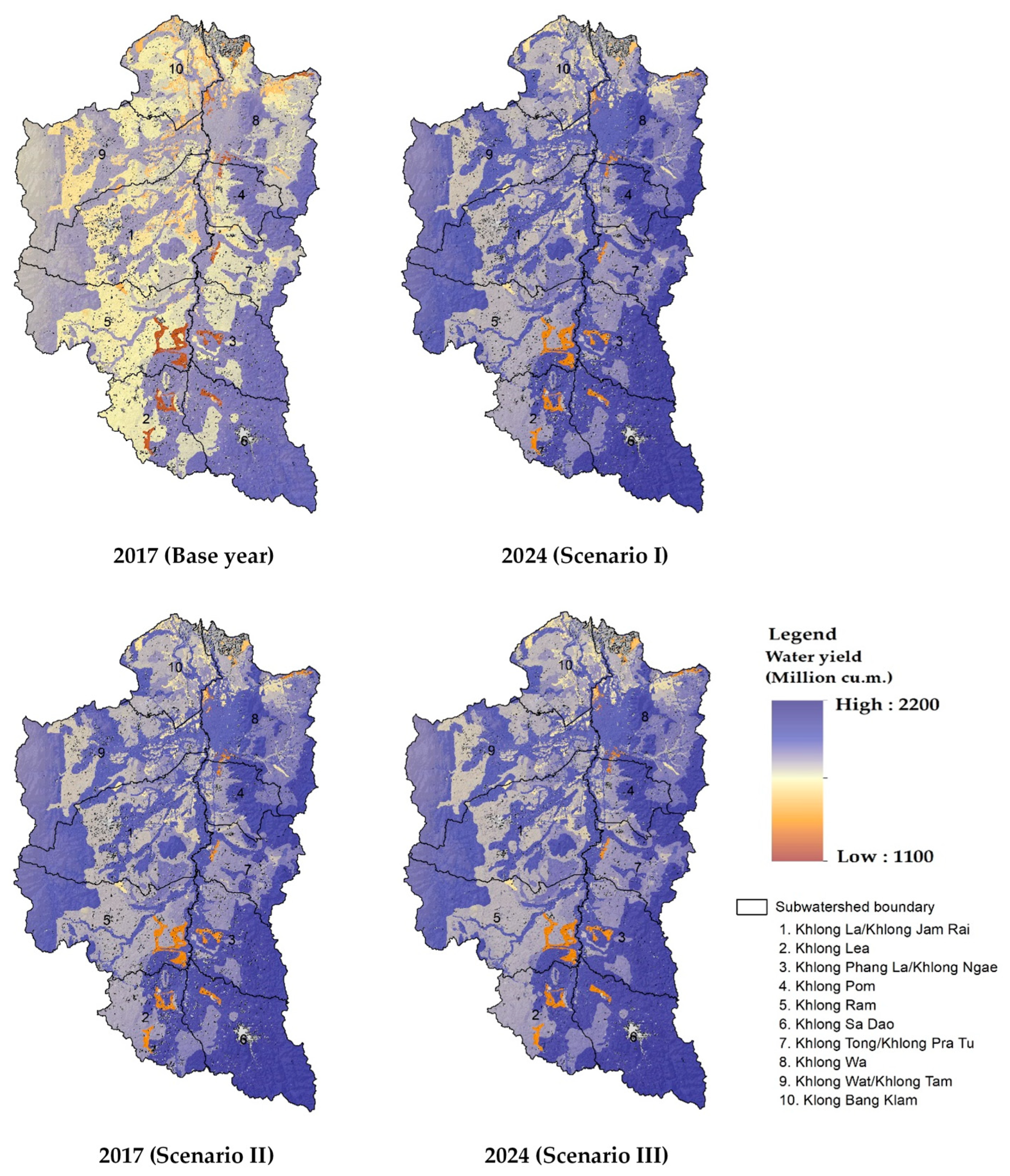
3.3. Water Yield Ecosystem Service Assessment

Based on LULC data in 2017, total water yield (runoff) was 1,863.80 mil. m³. Meanwhile, the predictive LULC data between 2018 and 2024 of Scenario I will generate the lowest average water yield than Scenario II and III with average value of 1,746.89 mil. m³ (

Table 6. Estimation of water yield of three different scenarios between 2018 and 2024.

Year	Annual Rainfall	Water Yield (mil. m3)
	(mm)	Scenario I	Scenario II	Scenario III
2018	2406.08	1,755,154,110.51	1,755,799,564.77	1,756,375,718.37
2019	2221.32	1,616,257,946.91	1,617,767,874.74	1,619,029,718.35
2020	2371.75	1,726,525,208.33	1,728,733,356.91	1,730,702,036.99
2021	2330.22	1,695,370,640.42	1,698,139,630.56	1,700,840,701.27
2022	2502.55	1,820,993,958.11	1,824,878,523.67	1,828,995,825.16
2023	2462.50	1,790,466,081.66	1,795,291,837.77	1,799,989,836.18
2024	2509.89	1,823,490,354.39	1,829,037,584.00	1,834,815,601.78
Average	2400.62	1,746,894,042.90	1,749,949,767.49	1,752,964,205.44

). Since LULC of Scenario I does not represent dramatic LULC change. The contribution of each LULC type on water yield is insignificant. Herewith, major increasing LULC classes under this scenario were urban and built-up area, rubber plantation, oil palm plantation while minor decreasing LULC classes were paddy field, evergreen forest, marsh and swamp, and miscellaneous land. In contrast, LULC of Scenario II and III were predicted based on the transformation of government policy in forestry and agriculture, respectively. The contribution of LULC from Scenario II and III highly reflects on water yield (runoff) than Scenario I. Under Scenario II, major increasing LULC classes were urban and built-up area, oil palm plantation, and evergreen forest; major decreasing LULC classes were rubber plantation and miscellaneous land during 2018–2024. Likewise, major increasing LULC classes under Scenario III, were urban and built-up area and oil palm plantation, and decreasing LULC classes were rubber plantation and marsh and miscellaneous land in the same periods. Additionally, Scenario III will generate the highest annual water yield than Scenario I and II with an average value of 1,752.96 mil.m³ (Table 6). Spatial distribution of water yield in 2017 and 2024 of three different scenarios are displayed in Figure 5.

In addition, the validation result of water yield estimation with observed data from the hydrological station of the Royal Irrigation Department at X90 (Khlong U-Tapao) during 2010–2017 provided an excellent fit with NSE of 0.81 and R² of 0.87 as mentioned by Reference [63].

3.4. Sediment Retention Ecosystem Service Assessment

Based on LULC data in 2017, the average annual soil loss was 10,293.19 tons/km². Meanwhile, the predictive LULC data between 2018 and 2024 of Scenario I will generate the highest annual erosion than Scenario II and III with an average value of 9,609.39 tons/km². In contrast, Scenario II will generate the lowest annual soil erosion than Scenario I and III with an average value of 8,403.54 tons/km² (

Table 7. Estimation of soil erosion, sediment retention, and sediment export of three different scenarios between 2018 and 2024.

Year	Soil Erosion (tons/km2)			Sediment Retention (tons/km2)			Sediment Export (tons/km2)
	Scenario I	Scenario II	Scenario III	Scenario I	Scenario II	Scenario III	Scenario I	Scenario II	Scenario III
2018	9541.79	9166.44	9352.96	3310.83	3314.86	3313.82	219.60	204.65	208.52
2019	8850.74	8215.66	8578.79	3053.91	3060.66	3058.07	206.75	181.75	191.32
2020	9445.76	8472.76	9076.33	3235.46	3245.68	3240.85	222.12	184.25	202.15
2021	9334.90	8127.66	8866.48	3221.15	3233.53	3227.32	220.84	174.99	197.99
2022	10,066.07	8519.22	9380.56	3487.20	3502.96	3495.42	240.05	181.68	209.58
2023	9891.33	8174.51	9169.52	3391.58	3409.01	3400.00	236.47	171.92	205.31
2024	10,135.12	8148.53	9226.04	3454.56	3474.59	3464.58	243.75	169.57	206.65
Average	9609.39	8403.54	9092.96	3307.81	3320.18	3314.29	227.08	181.26	203.07

). Likewise, the average annual sediment retention in 2017 was 2,892.58 tons/km². In the meantime, the predictive LULC between 2018 and 2024 of Scenario II will retain the highest annual sediment retention than Scenario I and III with an average value of 3,320.18 tons/km² since Scenario II will generate the lowest soil erosion than other scenarios. On the contrary, the predictive LULC of Scenario I will retain the lowest annual sediment retention than Scenario II and III with an average value of 3,307.81 tons/km² (Table 7). Similarly, average annual sediment export in 2017 was 227.40 tons/km². Meanwhile, the predictive LULC between 2018 and 2024 of Scenario II will deliver the lowest annual sediment export than Scenario I and III with an average value of 181.26 tons/km² since Scenario II will retain the highest sediment retention than other scenarios. On the contrary, the predictive LULC of Scenario I will deliver the highest annual sediment export than Scenario II and III with an average value of 227.08 tons/km² (Table 7). Spatial distribution of sediment retention in 2017 and 2024 of three different scenarios is displayed in Figure 6.

In addition, the validation result of the sediment export estimation with observed data from the hydrological station of the Royal Irrigation Department at X90 (Khlong U-Tapao) during 2011–2017 provided a good fit with NSE of 0.66 and R² of 0.82 [63].

3.5. LULC Scenario Identification for Optimum Water Yield and Soil Retention Ecosystem Services

The calculated average ESCI values of water yield (runoff) and sediment retention ecosystem services from three different LULC scenarios were simultaneously compared to identify the LULC scenario for optimum water yield (runoff) and sediment retention ecosystem services as summarized in

Table 8. Average ESCI values of the ecosystem service on water yield and sediment retention service among three different scenarios.

Period	Ecosystem Change Services Index (ESCI)
	Scenario I			Scenario II			Scenario III
	Water Yield	Sediment Retention	Average	Water Yield	Sediment Retention	Average	Water Yield	Sediment Retention	Average
2017–2018	−0.0583	0.1449	0.0433	−0.0579	0.1460	0.0441	−0.0576	0.1456	0.0440
2017–2019	−0.1328	0.0561	−0.0384	−0.1320	0.0581	−0.0370	−0.1313	0.0572	−0.0371
2017–2020	−0.0737	0.1188	0.0226	−0.0725	0.1221	0.0248	−0.0714	0.1204	0.0245
2017–2021	−0.0904	0.1139	0.0118	−0.0889	0.1179	0.0145	−0.0874	0.1157	0.0142
2017–2022	−0.0230	0.2059	0.0915	−0.0209	0.2110	0.0951	−0.0187	0.2084	0.0949
2017–2023	−0.0393	0.1728	0.0668	−0.0368	0.1785	0.0709	−0.0342	0.1754	0.0706
2017–2024	−0.0216	0.1946	0.0865	−0.0186	0.2012	0.0913	−0.0155	0.1977	0.0911
Average			0.0406			0.0434			0.0432

. As a result, average cumulative ESCI values of water yield (runoff) and sediment retention ecosystem services from LULC of Scenario II can provide the highest average ESCI value of 0.0434 among three different LULC scenarios. Therefore, LULC of Scenario II was chosen for optimum water yield (runoff) and sediment retention ecosystem services in Khlong U-Tapao watershed. This LULC scenario can mitigate flooding events in Khlong U-Tapao watershed and reduce sediment export in Songkhla Lake.

4. Discussion

4.1. LULC Assessment, Change, and Trend

Para-rubber trees, which are an economic tree of farmers in the Southern region of Thailand, had been increased during 2010–2017 and tended to increase in the near future according to the transitional probability of the Markov Chain. The observation is consistent with the previous study of Reference [37] which found forest land at Watershed Class I of U-Tapao watershed has been converted to rubber plantations. Likewise, Reference [39] mentioned that deforestation that has taken place in the SLB is converted into rubber plantations. Meanwhile, evergreen forests, which mostly situate on steep slopes, have been encroached for rubber plantations. Nevertheless, the prices of unsmoked rubber sheets grade III have a tendency to decline since it reaches the highest record in 2011 with 132.43 Baht/kg [64]. Additionally, the Thai Government encourages farmers to convert rubber to oil palm plantation [65] and reclaims forest areas back from intruders by law enforcement [61]. These imply that deforestation may tend to decrease in Klong U-Tapao watershed.

Besides, the classified LULC map from Landsat–TM and OLI using the RF classifier can provide overall accuracy and Kappa hat coefficient more than 80% that represents strong agreement or accuracy between the classified map and the reference map [66]. Additionally. These accuracy results are consistent with previous studies of [67,68,69,70]. However, to apply the RF model under the EnMap BOX software, users are required to observe the preliminary LULC result and add more training sample points to increase the accuracy of classification as mentioned by Reference [71].

4.2. LULC Prediction by CLUE-S Model

As results of LULC prediction by the CLUE-S model, the predicted LULC data in three different scenarios can provide realistic results as expectation. The deviation values between the required land area and the predicted area of each LULC type under three different scenarios are very small and vary from −0.1008% to 0.1290% or −10.08 km² (underestimation) to 12.89 km² (overestimation). In fact, the deviation value depends on iteration driving factors of each LULC type which indicates the maximum different allowance between the required and allocated area of LULC type under CLUE-S model [72,73,74]. Moreover, the derived AUC values for each LULC type allocation using binomial logit regression analysis exhibit good fit (0.7239) and excellent fit (0.9957) between the predicted and real LULC transition as mentioned by Reference [75]. These results imply that selected 8 driving factors on LULC change include elevation, slope, soil fertility, distance to road, distance to settlement, distance to water bodies, population density at the sub-district level, and average household income at the sub-district level are appropriate to apply for each LULC type allocation under CLUE-S model. In addition, distance to settlement, which is the most common driving factor for all LULC types allocation in the current study, is consistent with the previous study of References [31,76] who found the most common driving factor for all LULC types (except paddy field) in 9 protected forest areas in Phuket Island is distance to settlement.

Consequently, the CLUE-S model can be used as an efficient tool to predict LULC based on specific policies as the scenario. In practice, the optimum derived multiple linear equation from the binomial logit regression analysis for each LULC type allocation, land requirement of different scenarios (which are assigned by policy transformation), and model parameters (elasticity and LULC conversion matrix) are very important for predicting LULC under the CLUE-S model.

4.3. Water Yield Estimation

Dynamic pattern of water yield (runoff) in three different scenarios during 2018–2024 is dictated by annual rainfall data (see Table 6). It was found that there is a simple linear relationship between annual rainfall data during 2018–2024 as an independent variable and estimated water yield volume in the same period of each scenario as dependent variable provide the R² between 0.9992 and 0.9999. The significant difference of annual water yield volume of three different scenarios depends on predictive LULC change of three scenarios since annual rainfall data of three different scenarios are similar. The contribution of LULC from Scenario II and III highly reflect on water yield (runoff) than Scenario I. Reference [77] found that the conversion of an evergreen forest into rubber plantation and oil palm plantation affects the local hydrological cycle by decreasing infiltration and increasing the flooding frequency [77,78,79]. The evapotranspiration from evergreen forest in general generates lower water yields per unit area compared to the less forested in watershed areas [29].

4.4. Sediment Retention Estimation

Sediment dynamics at the catchment scale are mainly determined by climate, soil properties, topography, and vegetation, and anthropogenic factors, such as agricultural activities or dam construction and operation. Main sediment sources include overland erosion (soil particles detached and transported by rain and overland flow), gullies (channels that concentrate flow), bank erosion, and mass erosion [45]. As results of the study, it reveals that the predictive LULC between 2018 and 2024 of Scenario II can retain the highest annual sediment retention than Scenario I and Scenario III since it generates the lowest annual soil loss than other scenarios. This result indicates the influence of dynamic factor under RUSLE model of scenario includes cover factor (C) and practice factor for erosion control practice (P) from each LULC data scenario (see Appendix Table A3). In this study, Scenario II increases more evergreen forests than other scenarios. In fact, evergreen forest areas of Scenario II with value of 254.01 km² in 2017 will be 377.33 km² in 2024, while the area of evergreen forest of Scenario I and III will be 215.46 and 257.93 km² in 2024, respectively.

4.5. Optimum LULC Scenario for Ecosystem Services

By considering average cumulative ESCI values of water yield and sediment retention ecosystem services between base year (2017) and dynamic predictive LULC scenarios during 2018–2024, LULC scenario II was chosen for optimum water yield (runoff) and sediment retention ecosystem services in Khlong U-Tapao watershed.

However, when water yield and sediment retention ecosystem services were separately considered, LULC of Scenario I generates the least runoff in every year during 2018–2024 and the cumulative ESCI values on runoff ecosystem service of this scenario was also the lowest with average ESCI value of −0.0627. Thus, the LULC of Scenario I can be chosen for optimum water yield (runoff) ecosystem service to mitigate flood risk in Khlong U-Tapao watershed. In the meantime, the LULC of Scenario II retains the highest sediment retention in the same period and the cumulative ESCI values on sediment retention ecosystem service of this scenario were also the highest with an average of 0.1478. Therefore, LULC of Scenario II can be selected for the optimum sediment retention ecosystem service to reduce sediment export into Songkhla Lake.

5. Conclusions

Assessing the status and change of LULC between 2010 and 2017 was successfully implemented using digital image processing with the RF classifier and post-classification comparison change detection algorithm. The derived overall accuracy and Kappa hat coefficient of both LULC maps were more than 80%. In the meantime, the prediction of LULC change of three different scenarios during 2018–2024 was successfully simulated using the CLUE-S model. The predictive LULC data of three different scenarios provided realistic results, as expected. Then, the actual LULC in 2017 and predictive LULC during 2018–2024 and coupled with climate, soil and topography data were applied to evaluate ecosystem service in term of water yield and sediment retention using the Water Yield model and SDR models of InVEST. The validation results for water yield estimation with NSE of 0.81 and R² of 0.87 and sediment export estimation with NSE of 0.66 and R² of 0.82 were acceptable. Finally, the average cumulative ESCI values of water yield and sediment retention ecosystem services between base year (2017) and dynamic predictive LULC scenarios during 2018–2024 were calculated and compared to identify an optimum LULC scenario. As a result, LULC scenario II was selected for optimum water yield (runoff) and sediment retention ecosystem services.

In conclusion, the integration of remote sensing technology with advanced classification method (Random Forests) and geospatial models (CLUE-S model, Water Yield, and SDR models of InVEST) can be used as efficient tools to provide geospatial data on water yield and sediment retention ecosystem services from different scenarios. This research methodology framework can be used as a basic guideline for land use planners, land managers, or policymakers to evaluate the optimum LULC scenario for specific ecosystem services. However, the costs and benefits of the scenarios and implications in terms of a policy should be extensively considered in more detail.

References

1. Chiang, L.-C.; Chuang, Y.-T.; Han, C.-C. Integrating Landscape Metrics and Hydrologic Modeling to Assess the Impact of Natural Disturbances on Ecohydrological Processes in the Chenyulan Watershed, Taiwan. Int. J. Environ. Res. Public Health 2019, 16, 266. [Google Scholar] [CrossRef]
2. Tallis, H.T.; Ricketts, T.; Guerry, A.D.; Nelson, E.; Ennaanay, D.; Wolny, S.; Olwero, N.; Vigerstol, K.; Pennington, D.; Mendoza, G.; et al. InVEST 2.1 Beta User’s Guide: Integrated Valuation of Ecosystem Services and Tradeoff; Stanford University: Stanford, CA, USA, 2011. [Google Scholar]
3. Shoyama, K.; Yamagata, Y. Predicting land-use change for biodiversity conservation and climate-change mitigation and its effect on ecosystem services in a watershed in Japan. Ecosyst. Serv. 2014, 8, 25–34. [Google Scholar] [CrossRef]
4. Guardiola-Claramonte, M.; Troch, P.A.; Ziegler, A.D.; Giambelluca, T.W.; Durcik, M.; Vogler, J.B.; Nullet, M.A. Hydrologic effects of the expansion of rubber (Hevea brasiliensis) in a tropical catchment. Ecohydrology 2010, 3, 306–314. [Google Scholar] [CrossRef]
5. Hamilton, L.S. Forest and Water: A Thematic Study Prepared in the Frame-Work of the Global Forest Resources Assessment 2005; FAO: Rome, Italy, 2008. [Google Scholar]
6. Suryatmojo, H.; Fujimoto, M.; Yamakawa, Y.; Kosugi, K.I.; Mizuyama, T. Water balance changes in the tropical rainforest with intensive forest management system. Int. J. Sustain. Future Hum. Secur. 2013, 1, 56–62. [Google Scholar] [CrossRef]
7. Morgan, R.P.C. Soil Erosion and Conservation, 2nd ed.; Longman Group Ltd: Harlow, UK, 1995. [Google Scholar]
8. Gregersen, J.B.; Gijsbers, P.J.A.; Westen, S.J.P. OpenMI: Open modelling interface. J. Hydroinform. 2007, 9, 175–191. [Google Scholar] [CrossRef] [Green Version]
9. Dutta, S. Soil erosion, sediment yield and sedimentation of reservoir: A review. Model. Earth Syst. Environ. 2016, 2, 123. [Google Scholar] [CrossRef]
10. Hajigholizadeh, M.; Melesse, A.M.; Fuentes, H.R. Erosion and Sediment Transport Modelling in Shallow Waters: A Review on Approaches, Models and Applications. Int. J. Environ. Res. Public Health 2018, 15, 518. [Google Scholar] [CrossRef] [PubMed]
11. Boonkaewwan, S. Impacts of land-use changes on watershed discharge and water quality in a large intensive agricultural area in Thailand AU—Chotpantarat, Srilert. Hydrol. Sci. J. 2018, 63, 1386–1407. [Google Scholar] [CrossRef]
12. Wuttichaikitcharoen, P.; Babel, S.M. Principal Component and Multiple Regression Analyses for the Estimation of Suspended Sediment Yield in Ungauged Basins of Northern Thailand. Water 2014, 6, 2412–2435. [Google Scholar] [CrossRef] [Green Version]
13. Bogdan, S.-M.; Pătru-Stupariu, I.; Zaharia, L. The Assessment of Regulatory Ecosystem Services: The Case of the Sediment Retention Service in a Mountain Landscape in the Southern Romanian Carpathians. Procedia Environ. Sci. 2016, 32, 12–27. [Google Scholar] [CrossRef] [Green Version]
14. Wang, H.-W.; Kondolf, M.; Tullos, D.; Kuo, W.-C. Sediment Management in Taiwan’s Reservoirs and Barriers to Implementation. Water 2018, 10, 1034. [Google Scholar] [CrossRef]
15. Kondolf, G.M.; Gao, Y.; Annandale, G.W.; Morris, G.L.; Jiang, E.; Zhang, J.; Cao, Y.; Carling, P.; Fu, K.; Guo, Q.; et al. Sustainable sediment management in reservoirs and regulated rivers: Experiences from five continents. Earth’s Future 2014, 2, 256–280. [Google Scholar] [CrossRef]
16. Rahmani, V.; Kastens, J.H.; DeNoyelles, F.; Jakubauskas, M.E.; Martinko, E.A.; Huggins, D.H.; Gnau, C.; Liechti, P.M.; Campbell, S.W.; Callihan, R.A.; et al. Examining Storage Capacity Loss and Sedimentation Rate of Large Reservoirs in the Central U.S. Great Plains. Water 2018, 10, 190. [Google Scholar] [CrossRef]
17. Wohl, E.; Bledsoe, B.P.; Jacobson, R.B.; Poff, N.L.; Rathburn, S.L.; Walters, D.M.; Wilcox, A.C. The Natural Sediment Regime in Rivers: Broadening the Foundation for Ecosystem Management. BioScience 2015, 65, 358–371. [Google Scholar] [CrossRef] [Green Version]
18. Hamel, P.; Falinski, K.; Sharp, R.; Auerbach, D.A.; Sánchez-Canales, M.; Dennedy-Frank, P.J. Sediment delivery modeling in practice: Comparing the effects of watershed characteristics and data resolution across hydroclimatic regions. Sci. Total Environ. 2017, 580, 1381–1388. [Google Scholar] [CrossRef]
19. Han, X.; Lv, P.; Zhao, S.; Sun, Y.; Yan, S.; Wang, M.; Han, X.; Wang, X. The Effect of the Gully Land Consolidation Project on Soil Erosion and Crop Production on a Typical Watershed in the Loess Plateau. Land 2018, 7, 113. [Google Scholar] [CrossRef]
20. Gurung, K.; Yang, J.; Fang, L. Assessing Ecosystem Services from the Forestry-Based Reclamation of Surface Mined Areas in the North Fork of the Kentucky River Watershed. Forests 2018, 9, 652. [Google Scholar] [CrossRef]
21. Lane, L.J.; Nichols, M.H.; Levick, L.R.; Kidwell, M.R. A Simulation Model for Erosion and Sediment Yield at the Hillslope Scale. In Landscape Erosion and Evolution Modeling; Harmon, R.S., Doe, W.W., Eds.; Springer: Boston, MA, USA, 2001; pp. 201–237. [Google Scholar] [CrossRef]
22. Abdulkareem, J.H.; Pradhan, B.; Sulaiman, W.N.A.; Jamil, N.R. Prediction of spatial soil loss impacted by long-term land-use/land-cover change in a tropical watershed. Geosci. Front. 2019, 10, 389–403. [Google Scholar] [CrossRef]
23. Ahrends, A.; Hollingsworth, P.M.; Ziegler, A.D.; Fox, J.M.; Chen, H.; Su, Y.; Xu, J. Current trends of rubber plantation expansion may threaten biodiversity and livelihoods. Glob. Environ. Chang. 2015, 34, 48–58. [Google Scholar] [CrossRef]
24. Asari, N.; Suratman, M.N.; Jaafar, J. Modelling and mapping of above ground biomass (AGB) of oil palm plantations in Malaysia using remotely-sensed data. Int. J. Remote Sens. 2017, 38, 4741–4764. [Google Scholar] [CrossRef]
25. Razak, J.A.B.A.; Shariff, A.R.B.M.; Ahmad, N.B.; Ibrahim Sameen, M. Mapping rubber trees based on phenological analysis of Landsat time series data-sets. Geocarto Int. 2018, 33, 627–650. [Google Scholar] [CrossRef]
26. Ye, S.; Rogan, J.; Sangermano, F. Monitoring rubber plantation expansion using Landsat data time series and a Shapelet-based approach. ISPRS J. Photogramm. Remote Sens. 2018, 136, 134–143. [Google Scholar] [CrossRef]
27. Tian, S.; Zhang, X.; Tian, J.; Sun, Q. Random Forest Classification of Wetland Landcovers from Multi-Sensor Data in the Arid Region of Xinjiang, China. Remote Sens. 2016, 8, 954. [Google Scholar] [CrossRef]
28. Teluguntla, P.; Thenkabail, P.S.; Oliphant, A.; Xiong, J.; Gumma, M.K.; Congalton, R.G.; Yadav, K.; Huete, A. A 30-m landsat-derived cropland extent product of Australia and China using random forest machine learning algorithm on Google Earth Engine cloud computing platform. ISPRS J. Photogramm. Remote Sens. 2018, 144, 325–340. [Google Scholar] [CrossRef]
29. Trisurat, Y.; Eawpanich, P.; Kalliola, R. Integrating land use and climate change scenarios and models into assessment of forested watershed services in Southern Thailand. Environ. Res. 2016, 147, 611–620. [Google Scholar] [CrossRef] [PubMed]
30. Trisurat, Y.; Shirakawa, H.; Johnston, J.M. Land-Use/Land-Cover Change from Socio-Economic Drivers and Their Impact on Biodiversity in Nan Province, Thailand. Sustainability 2019, 11, 649. [Google Scholar] [CrossRef]
31. Ongsomwang, S.; Boonchoo, K. Integration of geospatial models for the allocation of deforestation hotspots and forest protection units. Suranaree J. Sci. Technol. 2016, 23, 283–307. [Google Scholar]
32. Verburg, P.H.; de Koning, G.H.J.; Kok, K.; Veldkamp, A.; Bouma, J. A spatial explicit allocation procedure for modelling the pattern of land use change based upon actual land use. Ecol. Model. 1999, 116, 45–61. [Google Scholar] [CrossRef]
33. Lüke, A.; Hack, J. Comparing the Applicability of Commonly Used Hydrological Ecosystem Services Models for Integrated Decision-Support. Sustainability 2018, 10, 346. [Google Scholar] [CrossRef]
34. Arunyawat, S.; Shrestha, R. Assessing Land Use Change and Its Impact on Ecosystem Services in Northern Thailand. Sustainability 2016, 8, 768. [Google Scholar] [CrossRef]
35. Leh, M.D.K.; Matlock, M.D.; Cummings, E.C.; Nalley, L.L. Quantifying and mapping multiple ecosystem services change in West Africa. Agric. Ecosyst. Environ. 2013, 165, 6–18. [Google Scholar] [CrossRef]
36. Ongsomwang, S.; Iamchuen, N. Integration of geospatial models for optimum land use allocation in three different scenarios. Suranaree J. Sci. Technol. 2015, 22, 19. [Google Scholar]
37. Doungsuwan, N.; Ratanachai, C.; Somgpongchaiyakul, P.; Sangganjanavanich, P. Impacts Of The National Economic And Social Development Plan On Songkhla Lake Basin Development Thailand. Int. Bus. Econ. Res. J. 2013, 12, 7. [Google Scholar] [CrossRef]
38. Department of Mineral Resources. Geochemical Survey and Soil Erosion in Lower Songkhla Lake Basin; Department of Mineral Resources: Bangkok, Thailand, 2008.
39. Gyawali, S.; Techato, K.; Yuangyai, C.; Musikavong, C. Assessment of Relationship between Land uses of Riparian Zone and Water Quality of River for Sustainable Development of River Basin, A Case Study of U-Tapao River Basin, Thailand. Procedia Environ. Sci. 2013, 17, 291–297. [Google Scholar] [CrossRef]
40. Van der Linden, S.; Rabe, A.; Held, M.; Jakimow, B.; Leitão, P.J.; Okujeni, A.; Schwieder, M.; Suess, S.; Hostert, P. The EnMAP-Box—A Toolbox and Application Programming Interface for EnMAP Data Processing. Remote Sens. 2015, 7, 11249. [Google Scholar] [CrossRef]
41. Breiman, L. Random Forests. Mach. Learn. 2001, 45, 5–32. [Google Scholar] [CrossRef] [Green Version]
42. Congalton, R.; Green, K. Assessing the Accuracy of Remotely Sensed Data; CRC Press: Boca Raton, FL, USA, 2009. [Google Scholar] [CrossRef]
43. Verburg, P.H.; Soepboer, W.; Veldkamp, A.; Limpiada, R.; Espaldon, V.; Mastura, S.S.A. Modeling the Spatial Dynamics of Regional Land Use: The CLUE-S Model. Environ. Manag. 2002, 30, 391–405. [Google Scholar] [CrossRef]
44. Verburg, P.H.; Overmars, K.P. Combining top-down and bottom-up dynamics in land use modeling: Exploring the future of abandoned farmlands in Europe with the Dyna-CLUE model. Landsc. Ecol. 2009, 24, 1167–1181. [Google Scholar] [CrossRef]
45. Sharp, R.; Tallis, H.T.; Ricketts, T.; Guerry, A.D.; Wood, S.A.; Chaplin-Kramer, R.; Nelson, E.; Ennaanay, D.; Wolny, S.; Olwero, N.; et al. InVEST 3.2.0 User’s Guide; The Natural Capital Project; Stanford University: Stanford, CA, USA; University of Minnesota: Minneapolis, MN, USA; The Nature Conservancy: Arlington County, VA, USA; World Wildlife Fund: Gland, Switzerland, 2015. [Google Scholar]
46. Thailand Meteorological Department. Climate Data (2000–2018) in Songkhla Province; Thai Meteorological Department: Songkhla, Thailand, 2018.
47. National Center for Atmospheric Research (NCAR). Climate System Model, June 2004 version 3.0; NCAR: Boulder, CO, USA, 2004. [Google Scholar]
48. Riahi, K.; Grubler, A.; Nakicenovic, N. Scenarios of long-term socio-economic and environmental development under climate stabilization. Technol. Forecast. Soc. Chang. 2007, 74, 887–935. [Google Scholar] [CrossRef]
49. Land Development Department. Soil Map of Songkhla Province.; Ministry of Agriculture and Cooperatives: Bangkok, Thailand, 2001.
50. Zhou, W.; Liu, G.; Pan, J.; Feng, X. Distribution of available soil water capacity in China. J. Geogr. Sci. 2005, 15, 3–12. [Google Scholar] [CrossRef]
51. Droogers, P.; Allen, R.G. Estimating Reference Evapotranspiration Under Inaccurate Data Conditions. Irrig. Drain. Syst. 2002, 16, 33–45. [Google Scholar] [CrossRef]
52. Renard, K.G.; Freimund, J.R. Using monthly precipitation data to estimate the R-factor in the revised USLE. J. Hydrol. 1994, 157, 287–306. [Google Scholar] [CrossRef]
53. Wischmeier, W.H.; Smith, D.D. Predicting Rainfall Erosion Losses—A Guide to Conservation Planning; USDA, Science and Education Administration: Hyattsville, MD, USA, 1978.
54. Arnoldus, H.M.J. An Approximation of the Rainfall Factor in the Universal Soil Loss Equation; John Wiley and Sons Ltd.: Chichester, UK, 1980; pp. 127–132. [Google Scholar]
55. Land Development Department. Soil Erosion in Thailand; Land Development Department, Ministry of Agriculture and Cooperatives: Bangkok, Thailand, 2000.
56. Borselli, L.; Cassi, P.; Torri, D. Prolegomena to sediment and flow connectivity in the landscape: A GIS and field numerical assessment. CATENA 2008, 75, 268–277. [Google Scholar] [CrossRef]
57. Vigiak, O.; Malagó, A.; Bouraoui, F.; Vanmaercke, M.; Obreja, F.; Poesen, J.; Habersack, H.; Fehér, J.; Grošelj, S. Modelling sediment fluxes in the Danube River Basin with SWAT. Sci. Total Environ. 2017, 599–600, 992–1012. [Google Scholar] [CrossRef]
58. Southern Region Irrigation Hydrology Center. Water Yield and Sedimentation; Southern Region Irrigation Hydrology Center: Phattalung, Thailand, 2018. [Google Scholar]
59. Hair, J.F.; Black, W.C.; Babin, B.J.; Anderson, R.E. Multivariate Data Analysis, 7th ed.; Pearson: Harlow, UK, 2013. [Google Scholar]
60. Rogerson, P. Statistical Methods for Geography: A Student’s Guide, 3rd ed.; SAGE: Los Angeles, CA, USA; London, UK, 2010. [Google Scholar]
61. Chan-o-cha, P. National Broadcast by PM Prayut Chan-o-cha. 11 March 2016. Available online: http://thaiembdc.org/2016/03/14/nb-by-pm-march-11-2016 (accessed on 10 October 2018).
62. Raksaseri, K. THAILAND: Firm on Protecting the Palm Oil Sector. Available online: http://www.aseannews.net/thailand-firm-protecting-palm-oil-sector/ (accessed on 23 May 2018).
63. Motovilov, Y.G.; Gottschalk, L.; Engeland, K.; Rodhe, A. Validation of a distributed hydrological model against spatial observations. Agric. For. Meteorol. 1999, 98–99, 257–277. [Google Scholar] [CrossRef]
64. Bank of Thailand. Manufacturing Production in the Southern Region. Available online: http://www2.bot.or.th/statistics/ReportPage.aspx?reportID=590&language=eng (accessed on 5 January 2018).
65. Ministry of Agriculture and Cooperatives. A Guide to the Management of Agricultural Production in Zoning; Ministry of Agriculture and Cooperatives: Bangkok, Thailand, 2014.
66. Fitzpatrick-Lins, K. Comparison of sampling procedures and data analysis for a land-use and land cover map. Photogramm. Eng. Remote Sens. 1981, 47, 343–351. [Google Scholar]
67. Rodriguez-Galiano, V.F.; Ghimire, B.; Rogan, J.; Chica-Olmo, M.; Rigol-Sanchez, J.P. An assessment of the effectiveness of a random forest classifier for land-cover classification. ISPRS J. Photogramm. Remote Sens. 2012, 67, 93–104. [Google Scholar] [CrossRef]
68. Li, M.; Im, J.; Beier, C. Machine learning approaches for forest classification and change analysis using multi-temporal Landsat TM images over Huntington Wildlife Forest. GISci. Remote Sens. 2013, 50, 361–384. [Google Scholar] [CrossRef]
69. Sakuma, A.; Kameyama, S.; Ono, S.; Kizuka, T.; Mikami, H. Mapping of Unused Agricultural Land Distribution Using Landsat 8 OLI Surface Reflectance Products in the Kushiro River Watershed. J. Remote Sens. Soc. Jpn. 2017, 37, 421–433. [Google Scholar] [CrossRef]
70. Nguyen, H.T.T.; Doan, T.M.; Radeloff, V. APPLYING RANDOM FOREST CLASSIFICATION TO MAP LAND USE/LAND COVER USING LANDSAT 8 OLI. Int. Arch. Photogramm. Remote Sens. Spat. Inf. Sci. 2018, XLII-3/W4, 363–367. [Google Scholar] [CrossRef] [Green Version]
71. Tatsumi, K.; Yamashiki, Y.; Torres, M.A.C.; Taipe, C.L.R. Crop classification of upland fields using Random forest of time-series Landsat 7 ETM+ data. Comput. Electron. Agric. 2015, 115, 171–179. [Google Scholar] [CrossRef]
72. van Asselen, S.; Verburg, P.H. Land cover change or land-use intensification: Simulating land system change with a global-scale land change model. Glob. Chang. Biol. 2013, 19, 3648–3667. [Google Scholar] [CrossRef]
73. Liu, W.; Luo, Q.; Li, J.; Wang, P.; Lu, H.; Liu, W.; Li, H. The effects of conversion of tropical rainforest to rubber plantation on splash erosion in Xishuangbanna, SW China. Hydrol. Res. 2013, 46, 168–174. [Google Scholar] [CrossRef]
74. Xu, L.; Li, Z.; Song, H.; Yin, H. Land-Use Planning for Urban Sprawl Based on the CLUE-S Model: A Case Study of Guangzhou, China. Entropy 2013, 15, 3490–3506. [Google Scholar] [CrossRef]
75. Pontius, R.G.; Schneider, L.C. Land-cover change model validation by an ROC method for the Ipswich watershed, Massachusetts, USA. Agric. Ecosyst. Environ. 2001, 85, 239–248. [Google Scholar] [CrossRef]
76. Boonchoo, K. Geospatial Models for Land Use and Land Cover Prediction and Deforestation Vulnerability Analysis in Phuket Island, Thailand. Ph.D Thesis, Suranaree University of Technology, Nakhon Ratchasima, Thailand, 2015. [Google Scholar]
77. Tarigan, S.; Wiegand, K.; Slamet, B. Minimum forest cover required for sustainable water flow regulation of a watershed: A case study in Jambi Province, Indonesia. Hydrol. Earth Syst. Sci. 2018, 22, 581–594. [Google Scholar] [CrossRef]
78. Comte, I.; Colin, F.; Whalen, J.K.; Grünberger, O.; Caliman, J.-P. Chapter three—Agricultural Practices in Oil Palm Plantations and Their Impact on Hydrological Changes, Nutrient Fluxes and Water Quality in Indonesia: A Review. In Advances in Agronomy; Sparks, D.L., Ed.; Academic Press: Cambridge, MA, USA, 2012; Volume 116, pp. 71–124. [Google Scholar]
79. Meijide, A.; Röll, A.; Fan, Y.; Herbst, M.; Niu, F.; Tiedemann, F.; June, T.; Rauf, A.; Hölscher, D.; Knohl, A. Controls of water and energy fluxes in oil palm plantations: Environmental variables and oil palm age. Agric. For. Meteorol. 2017, 239, 71–85. [Google Scholar] [CrossRef]
80. Canadell, J.; Jackson, R.B.; Ehleringer, J.B.; Mooney, H.A.; Sala, O.E.; Schulze, E.D. Maximum rooting depth of vegetation types at the global scale. Oecologia 1996, 108, 583–595. [Google Scholar] [CrossRef]
81. Philip, K.; Maxene, A.; Steve, S.; Stacey, W.; Ethan, F.; Gregg, M.; Juan Carlos, M.-S.; Françoise, B.; Landy Sabrina, C.; Jean Roudy, A.; et al. Baseline Ecological Inventory for Three Bays National Park, Haiti; The Nature Conservancy: Arlington County, VA, USA, 2016. [Google Scholar]
82. Allen, R.G.; Pereira, L.S.; Raes, D.; Smith, M. Crop Evapotranspiration Guidelines for Computing Crop Water Requirements; FAO Irrigation and Drainage: Rome, Italy, 1998. [Google Scholar]
Figure 1. Location of the Khlong U-Tapao watershed, Songkhla Province, Thailand.
Sustainability 11 02895 g001
Figure 2. Schematic workflow of research methodology.
Sustainability 11 02895 g002
Figure 3. Spatial distribution of LULC data in 2010 and 2017.
Sustainability 11 02895 g003
Figure 4. Spatial distribution of predictive LULC in 2024 of three different scenarios.
Sustainability 11 02895 g004
Figure 5. Spatial distribution of water yield in 2017 and 2024 of three different scenarios.
Sustainability 11 02895 g005
Figure 6. Spatial distribution of sediment retention in 2017 and 2024 of three different scenarios.
Sustainability 11 02895 g006