Ground Deformation Analysis Using InSAR and Backpropagation Prediction with Influencing Factors in Erhai Region, China


 , ,
, ,
Abstract
:1. Introduction
2. Study Area and Data Sets
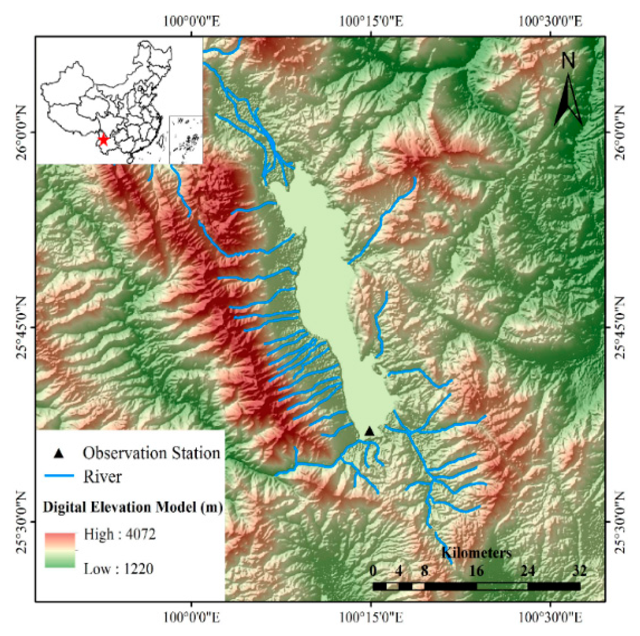
2.1. Study Area
2.2. Data Sets
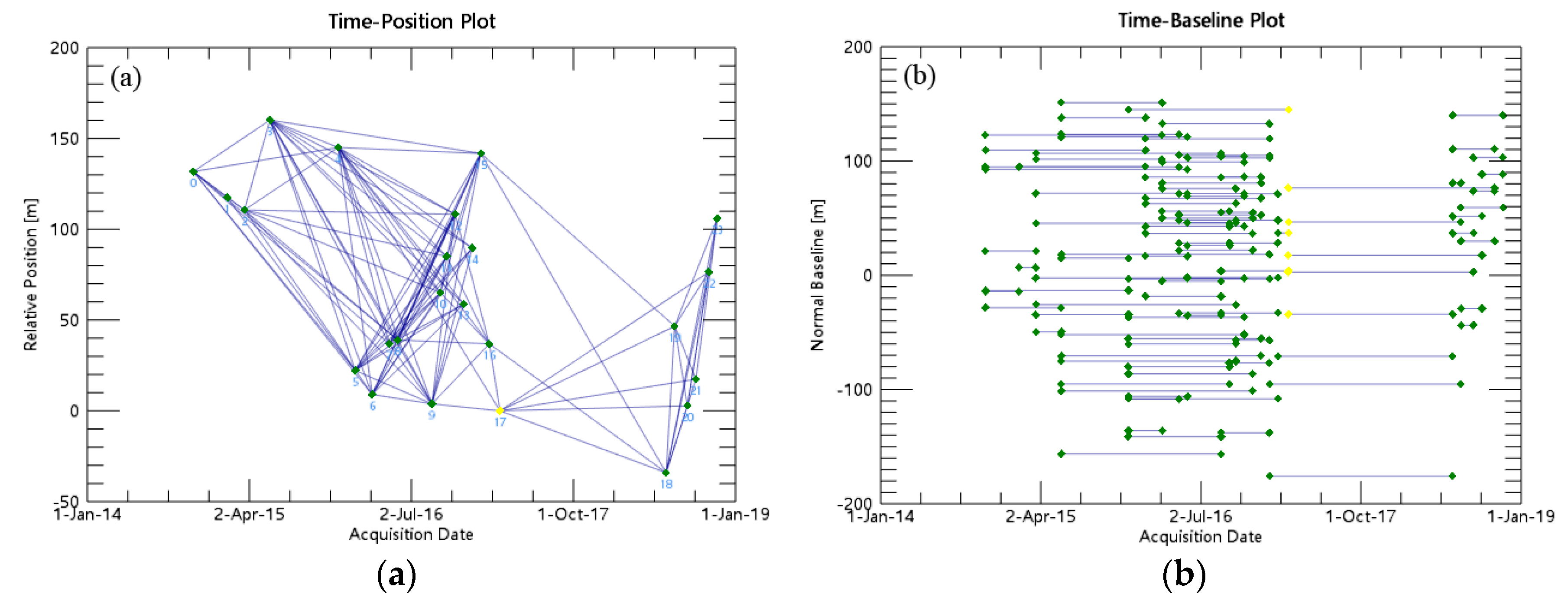
2.2.1. SAR Images
2.2.2. Landsat 8 Images
2.2.3. Temperature, Precipitation, and Water Level
3. Methodology of Processing
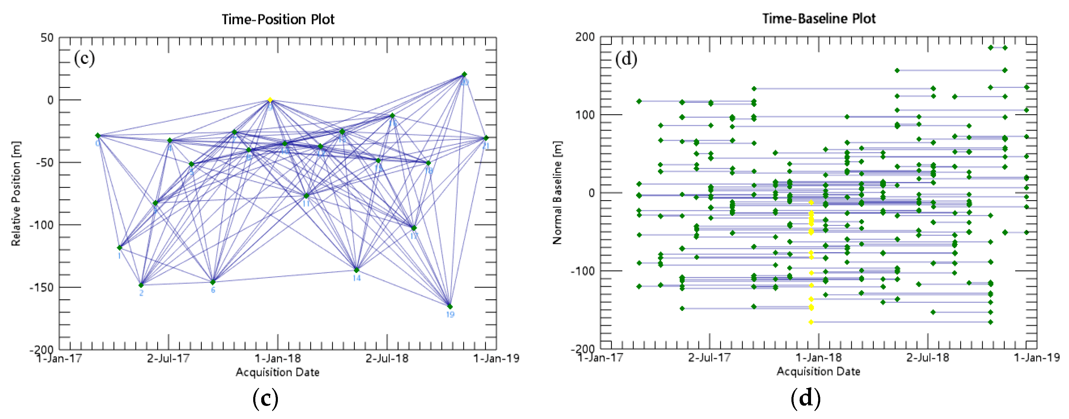
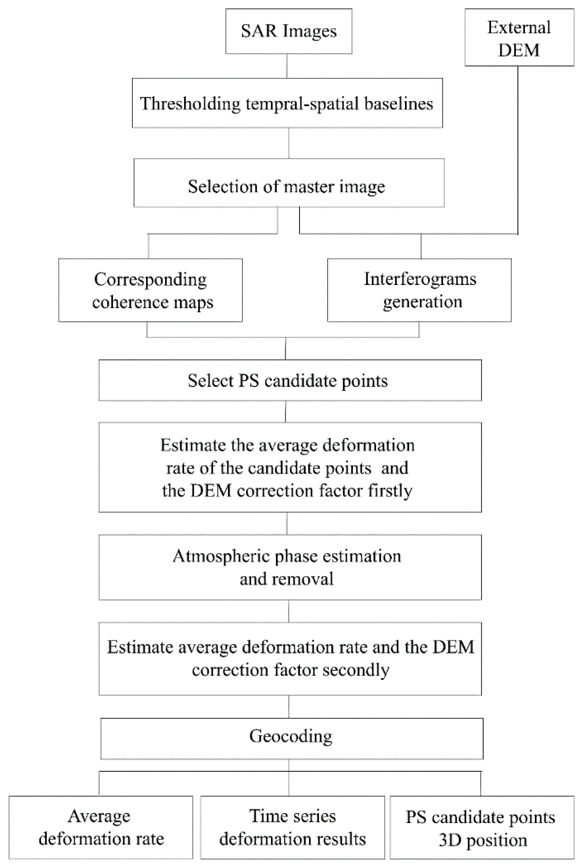
3.1. SBAS-InSAR Algorithm
3.2. Acquisition of Building Area
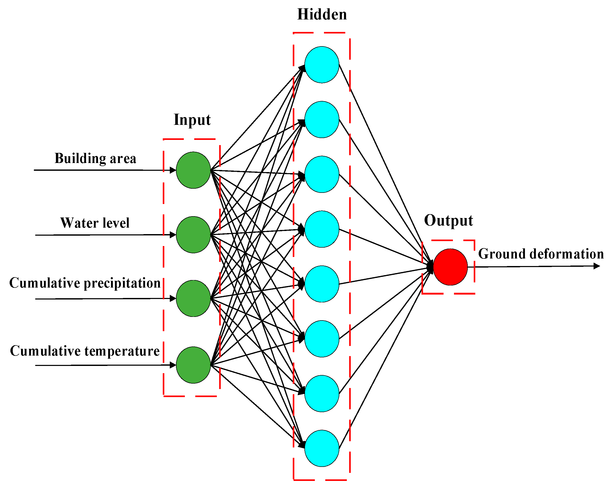
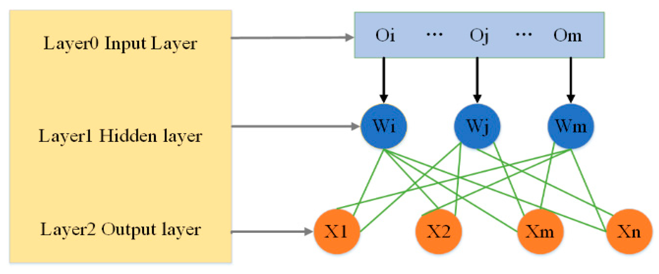
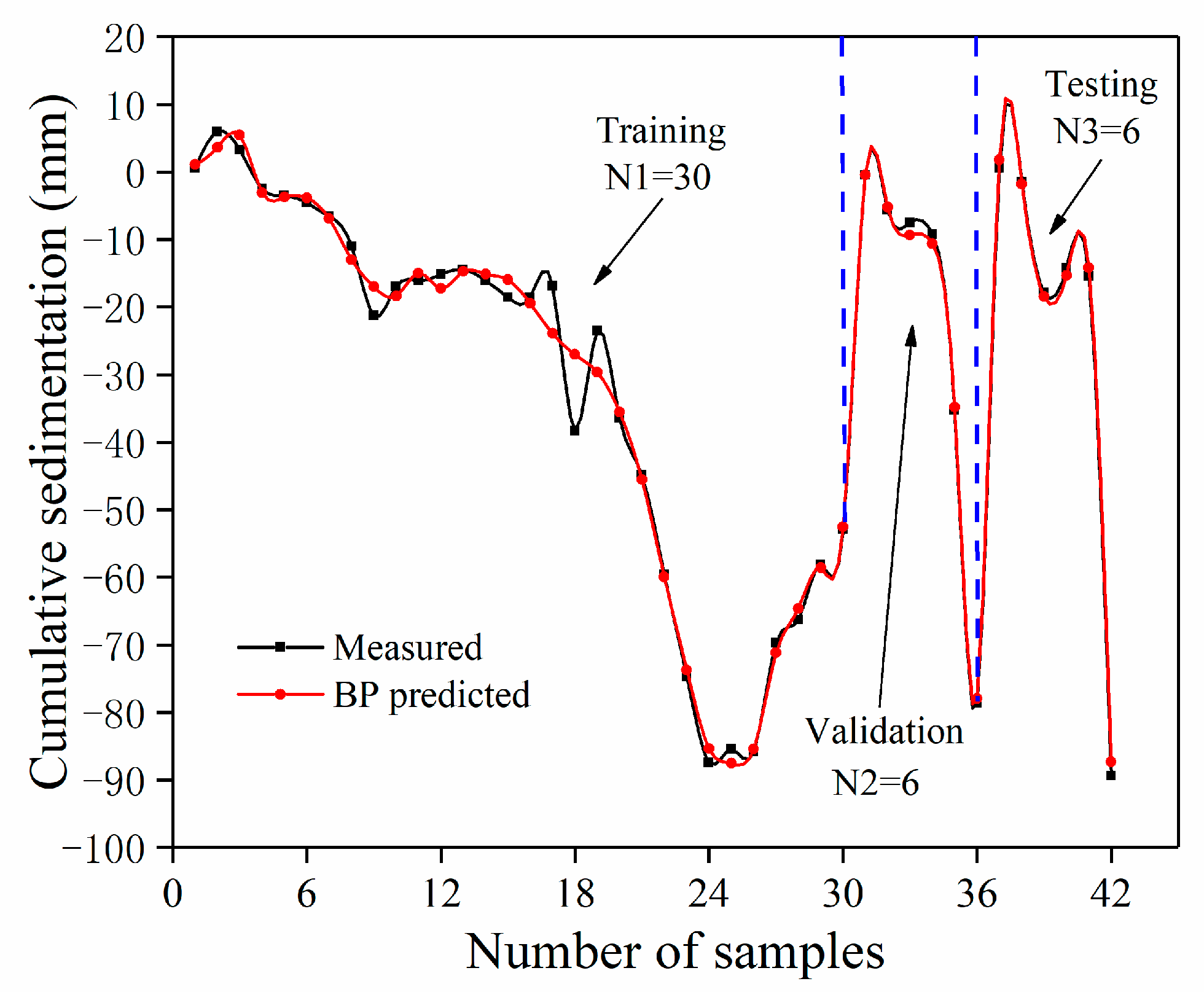
3.3. Predicting the Cumulative Ground Deformation Using Back-Propagation
4. Results
4.1. Deformation Results
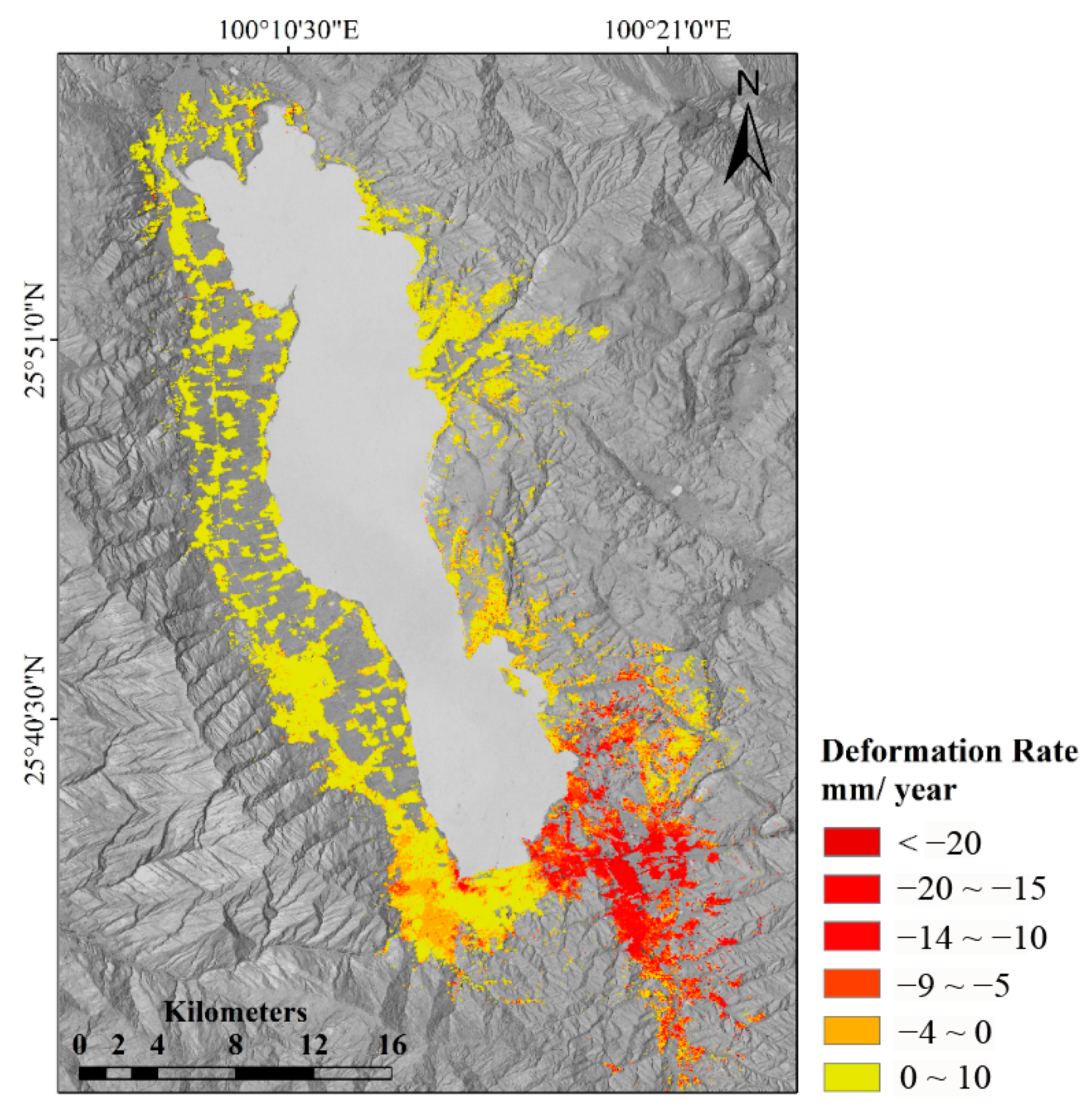
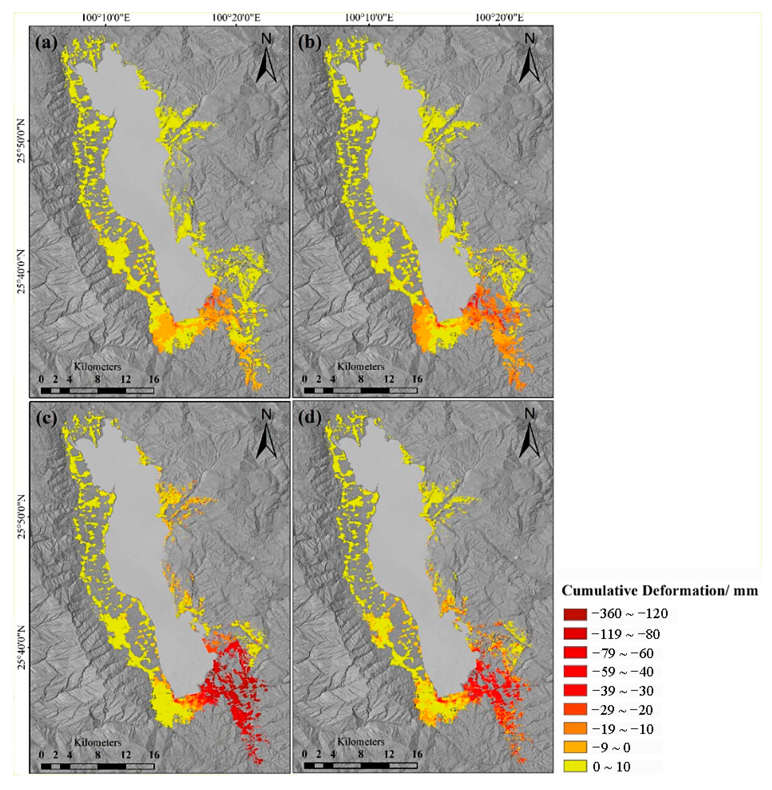
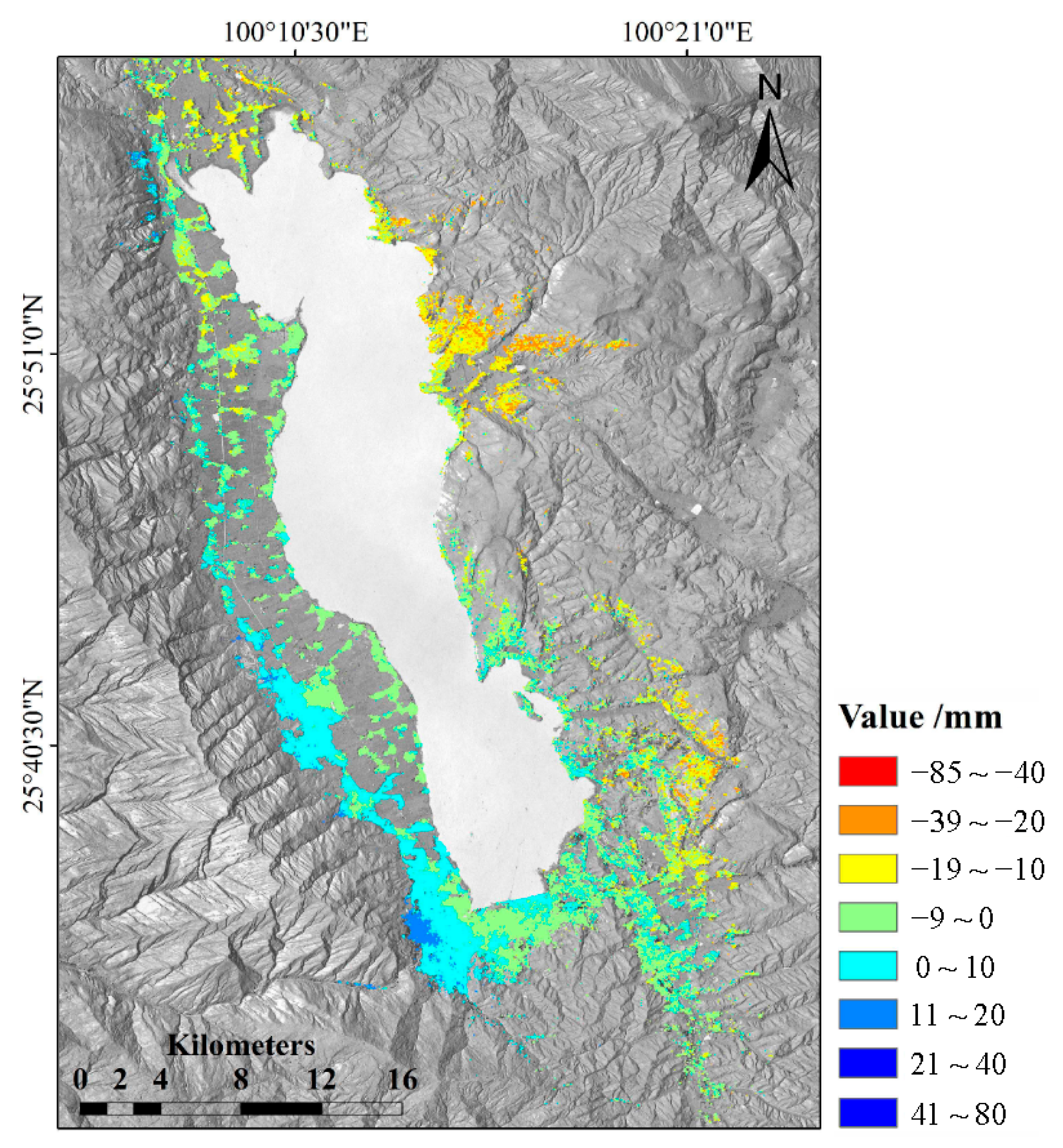
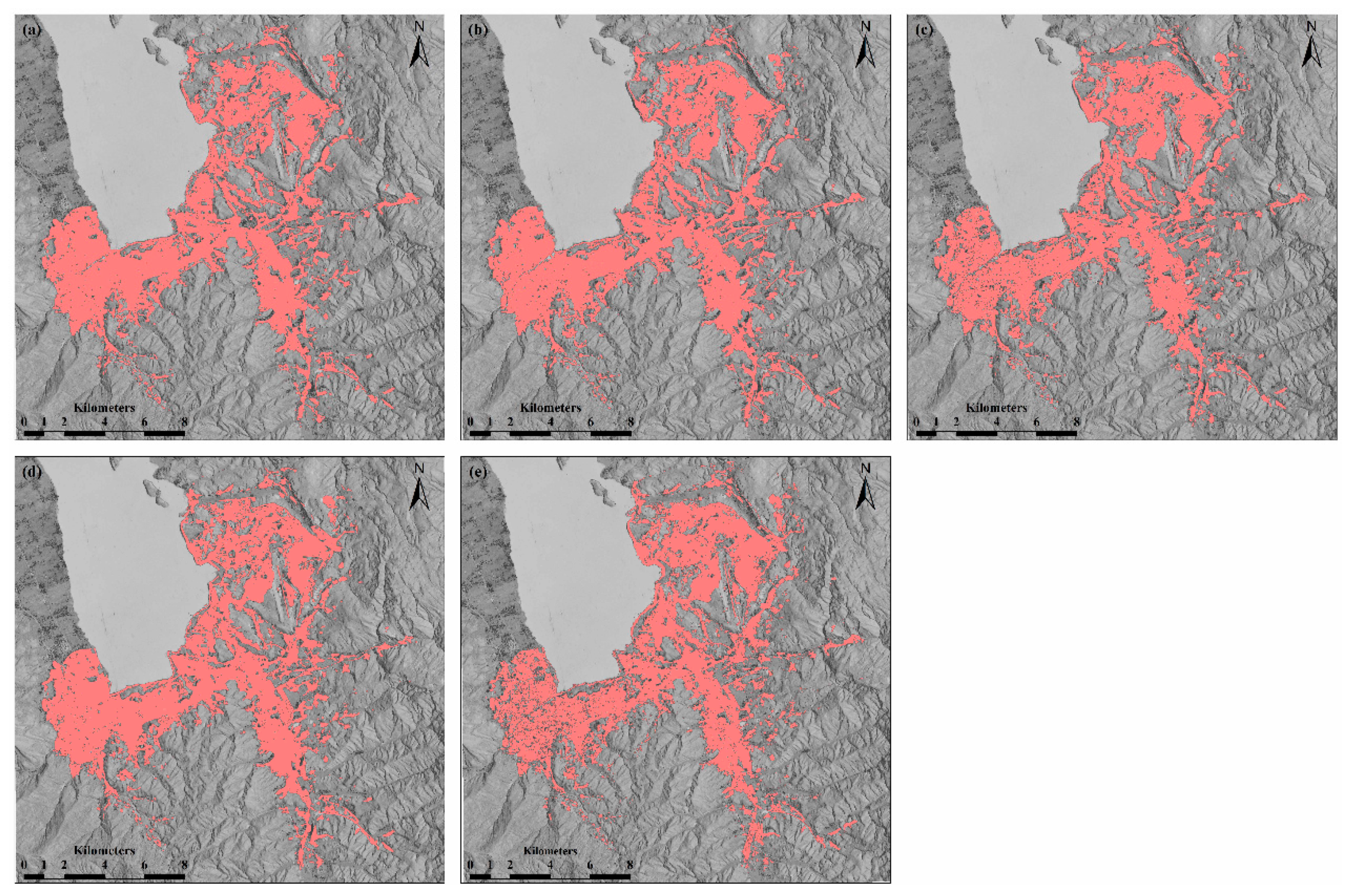
4.1.1. Mean Deformation Rate Map
4.1.2. Time Series of Deformation
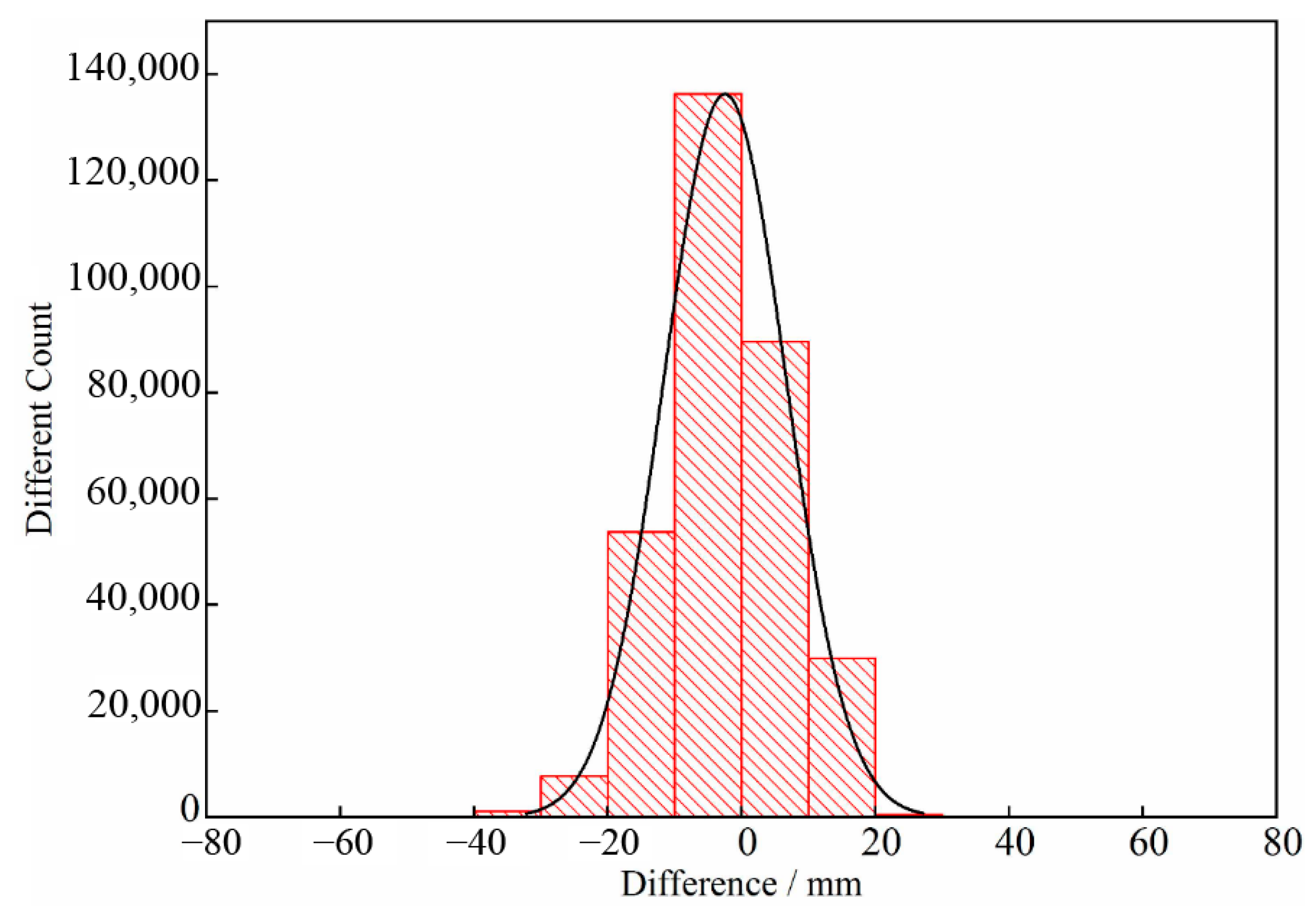
4.1.3. The Validation of Results
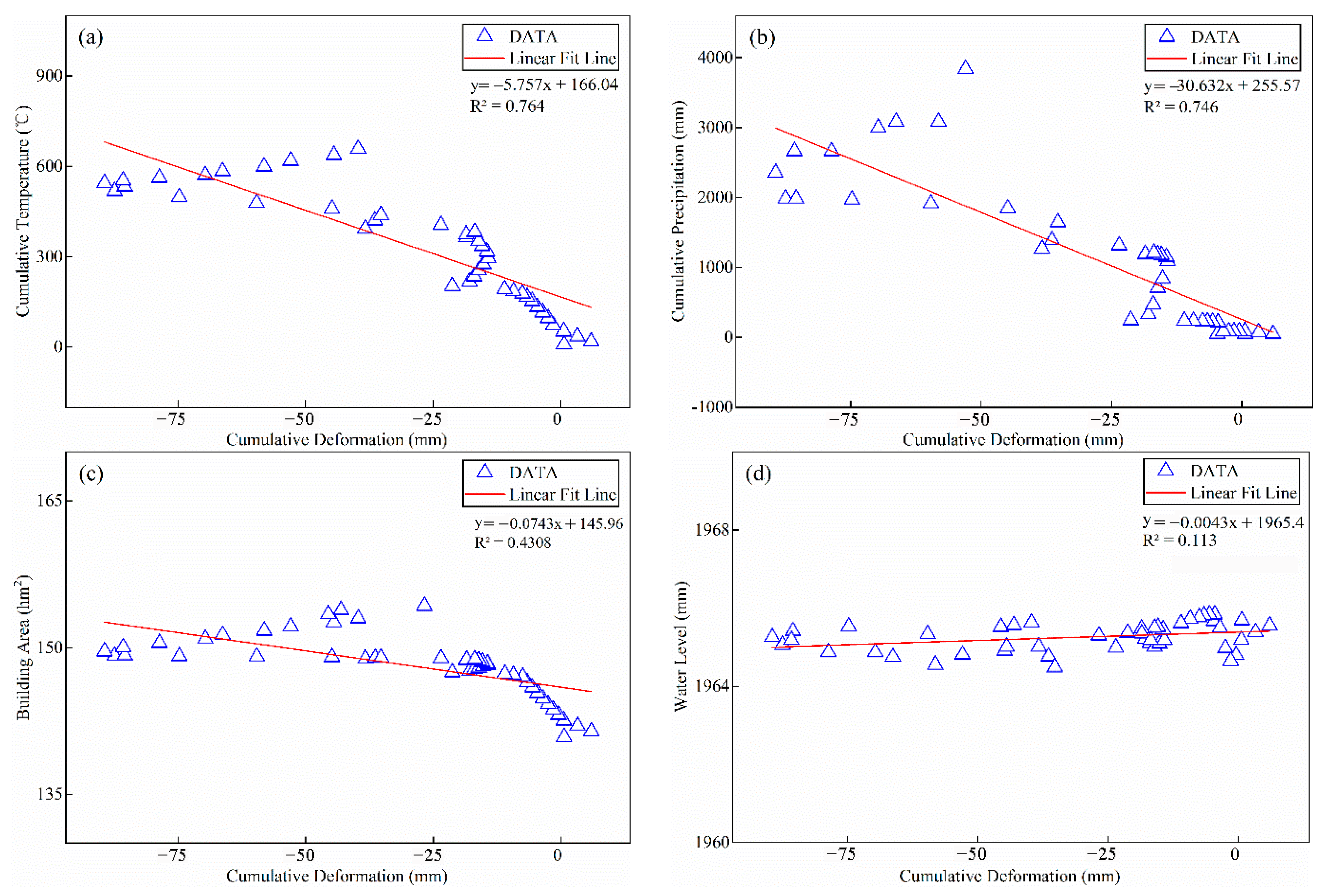
4.2. Correlation between Ground Deformation and Factors
4.2.1. Urbanization Rate of Dali City
4.2.2. Analysis of Influencing Factors to Ground Deformation
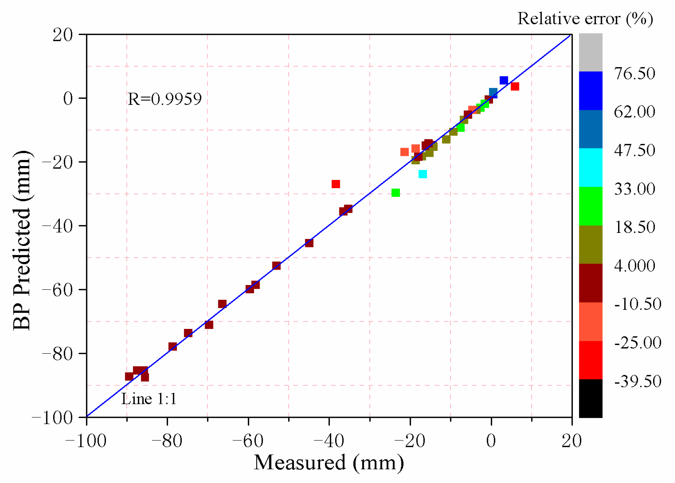
4.3. Results of Predicting the Cumulative Ground Deformation Using BP
5. Discussion
5.1. Deformation Results
5.2. Future Deformation Prediction
5.3. Countermeasures and Suggestions
6. Conclusions
Author Contributions
Funding
Acknowledgments
Conflicts of Interest
References
- Bekaert, D.P.; Jones, C.E.; An, K.; Huang, M.-H. Exploiting UAVSAR for a comprehensive analysis of subsidence in the Sacramento Delta. Remote Sens. Environ. 2019, 220, 124–134. [Google Scholar] [CrossRef]
- Gao, M.; Gong, H.; Chen, B.; Zhou, C.; Chen, W.; Liang, Y.; Shi, M.; Si, Y. InSAR time-series investigation of long-term ground displacement at Beijing Capital International Airport, China. Tectonophysics 2016, 691, 271–281. [Google Scholar] [CrossRef]
- Bell, F.G.; Stacey, T.R.; Genske, D.D. Mining subsidence and its effect on the environment: Some differing examples. Environ. Earth Sci. 2000, 40, 135–152. [Google Scholar] [CrossRef]
- Alloy, A.; Gonzalez Dominguez, F.; Nila Fonseca, A.L.; Ruangsirikulchai, A.; Gentle, J.N., Jr.; Cabral, E.; Pierce, S.A. Development of an expert analysis tool based on an interactive subsidence hazard map for urban land use in the city of Celaya, Mexico. In AGU Fall Meeting Abstracts; American Geophysical Union: Washington, DC, USA, 2016. [Google Scholar]
- Stramondo, S.; Bozzano, F.; Marra, F.; Wegmuller, U.; Cinti, F.; Moro, M.; Saroli, M. Subsidence induced by urbanisation in the city of Rome detected by advanced InSAR technique and geotechnical investigations. Remote Sens. Environ. 2008, 112, 3160–3172. [Google Scholar] [CrossRef]
- Castellazzi, P.; Arroyo-Domínguez, N.; Martel, R.; Calderhead, A.I.; Normand, J.C.; Gárfias, J.; Rivera, A. Land subsidence in major cities of Central Mexico: Interpreting InSAR-derived land subsidence mapping with hydrogeological data. Int. J. Appl. Earth Obs. Geoinf. 2016, 47, 102–111. [Google Scholar] [CrossRef]
- Huanhuan, L.; Youquan, Z.; Rong, W. The reason of land subsidence and prevention measures of Beijing segment of Beijing-Tianjin high-speed rail. In Proceedings of the 2014 Third International Workshop on Earth Observation and Remote Sensing Applications (EORSA), Changsha, China, 11–14 June 2014; pp. 323–325. [Google Scholar]
- Yang, C.-S.; Zhang, Q.; Zhao, C.-Y.; Wang, Q.-L.; Ji, L.-Y. Monitoring land subsidence and fault deformation using the small baseline subset InSAR technique: A case study in the Datong Basin, China. J. Geodyn. 2014, 75, 34–40. [Google Scholar] [CrossRef]
- Ng, A.H.-M.; Ge, L.; Li, X.; Zhang, K. Monitoring ground deformation in Beijing, China with persistent scatterer SAR interferometry. J. Geodyn. 2012, 86, 375–392. [Google Scholar] [CrossRef]
- Kim, J.-W.; Lu, Z.; Jia, Y.; Shum, C. Ground subsidence in Tucson, Arizona, monitored by time-series analysis using multi-sensor InSAR datasets from 1993 to 2011. ISPRS J. Photogramm. Sens. 2015, 107, 126–141. [Google Scholar] [CrossRef]
- Sharma, P.; Jones, C.E.; Dudas, J.; Bawden, G.W.; Deverel, S. Monitoring of subsidence with UAVSAR on Sherman Island in California’s Sacramento–San Joaquin Delta. Remote Sens. Environ. 2016, 181, 218–236. [Google Scholar] [CrossRef]
- Ying, M.; Zhang, W.; Yu, H.; Lu, X.; Feng, J.; Fan, Y.; Zhu, Y.; Chen, D. An Overview of the China Meteorological Administration Tropical Cyclone Database. J. Atmos. Ocean. Technol. 2014, 31, 287–301. [Google Scholar] [CrossRef]
- Massonnet, D.; Feigl, K.L. Radar interferometry and its application to changes in the Earth’s surface. Rev. Geophys. 1998, 36, 441–500. [Google Scholar] [CrossRef]
- Colesanti, C.; Ferretti, A.; Novali, F.; Prati, C.; Rocca, F. Sar monitoring of progressive and seasonal ground deformation using the permanent scatterers technique. IEEE Trans. Geosci. Sens. 2003, 41, 1685–1701. [Google Scholar] [CrossRef]
- Cascini, L.; Peduto, D.; Réale, D.; Arena, L.; Ferlisi, S.; Verde, S.; Fornaro, G. Detection and monitoring of facilities exposed to subsidence phenomena via past and current generation SAR sensors. J. Geophys. Eng. 2013, 10, 64001. [Google Scholar] [CrossRef]
- Amighpey, M.; Arabi, S. Studying land subsidence in Yazd province, Iran, by integration of InSAR and levelling measurements. Sens. Appl. Soc. 2016, 4, 1–8. [Google Scholar] [CrossRef]
- Rosen, P.A.; Hensley, S.; Joughin, I.R.; Li, F.K.; Madsen, S.N.; Rodriguez, E.; Goldstein, R.M. Synthetic aperture radar interferometry. Proc. IEEE 2002, 88, 333–382. [Google Scholar] [CrossRef]
- Atzori, S.; Hunstad, I.; Chini, M.; Salvi, S.; Tolomei, C.; Bignami, C.; Stramondo, S.; Trasatti, E.; Antonioli, A.; Boschi, E. Finite fault inversion of DInSAR coseismic displacement of the 2009 L’Aquila earthquake (central Italy). Geophys. Lett. 2009, 36. [Google Scholar] [CrossRef]
- Ge, L.; Chang, H.-C.; Rizos, C. Mine Subsidence Monitoring Using Multi-source Satellite SAR Images. Photogramm. Eng. Sens. 2007, 73, 259–266. [Google Scholar] [CrossRef]
- Trasatti, E.; Casu, F.; Giunchi, C.; Pepe, S.; Solaro, G.; Tagliaventi, S.; Berardino, P.; Manzo, M.; Pepe, A.; Ricciardi, G.P.; et al. The 2004-2006 uplift episode at Campi Flegrei caldera (Italy): Constraints from SBAS-DInSAR ENVISAT data and Bayesian source inference. Geophys. Lett. 2008, 35. [Google Scholar] [CrossRef]
- Ding, R.; Xu, J.; Lin, X.; Xu, K. Monitoring of surface subsidence using PSInSAR with TerraSAR-X high resolution data. Remote Sens. Land Resour. 2015, 27, 158–164. [Google Scholar]
- Canova, F.; Tolomei, C.; Salvi, S.; Toscani, G.; Seno, S. Land subsidence along the Ionian coast of SE Sicily (Italy), detection and analysis via Small Baseline Subset (SBAS) multitemporal differential SAR interferometry. Earth Surf. Process. Landf. 2012, 37, 273–286. [Google Scholar] [CrossRef]
- Lanari, R.; Casu, F.; Manzo, M.; Lundgren, P. Application of the SBAS-DInSAR technique to fault creep: A case study of the Hayward fault, California. Remote Sens. Environ. 2007, 109, 20–28. [Google Scholar] [CrossRef]
- Tizzani, P.; Berardino, P.; Casu, F.; Euillades, P.; Manzo, M.; Ricciardi, G.; Zeni, G.; Lanari, R. Surface deformation of Long Valley caldera and Mono Basin, California, investigated with the SBAS-InSAR approach. Remote Sens. Environ. 2007, 108, 277–289. [Google Scholar] [CrossRef]
- Zhao, R.; Li, Z.-W.; Feng, G.-C.; Wang, Q.-J.; Hu, J. Monitoring surface deformation over permafrost with an improved SBAS-InSAR algorithm: With emphasis on climatic factors modeling. Remote Sens. Environ. 2016, 184, 276–287. [Google Scholar] [CrossRef]
- Gee, D.; Sowter, A.; Novellino, A.; Marsh, S.; Gluyas, J. Monitoring land motion due to natural gas extraction: Validation of the Intermittent SBAS (ISBAS) DInSAR algorithm over gas fields of North Holland, the Netherlands. Mar. Pet. Geol. 2016, 77, 1338–1354. [Google Scholar] [CrossRef]
- Manunta, M.; Marsella, M.; Zeni, G.; Sciotti, M.; Atzori, S.; Lanari, R. Two-scale surface deformation analysis using the SBAS-DInSAR technique: A case study of the city of Rome, Italy. Int. J. Sens. 2008, 29, 1665–1684. [Google Scholar] [CrossRef]
- Zeni, G.; Bonano, M.; Casu, F.; Manunta, M.; Manzo, M.; Marsella, M.; Pepe, A.; Lanari, R. Long-term deformation analysis of historical buildings through the advanced SBAS-DInSAR technique: The case study of the city of Rome, Italy. J. Geophys. Eng. 2011, 8, S1–S12. [Google Scholar] [CrossRef]
- Dong, S.; Samsonov, S.; Yin, H.; Ye, S.; Cao, Y.J. Time-series analysis of subsidence associated with rapid urbanization in Shanghai, China measured with SBAS InSAR method. Environ. Earth Sci. 2014, 72, 677–691. [Google Scholar] [CrossRef]
- Xu, B.; Feng, G.; Li, Z.-W.; Wang, Q.; Wang, C.; Xie, R. Coastal Subsidence Monitoring Associated with Land Reclamation Using the Point Target Based SBAS-InSAR Method: A Case Study of Shenzhen, China. Remote Sens. 2016, 8, 652. [Google Scholar] [CrossRef]
- Zhou, L.; Guo, J.; Hu, J.; Li, J.; Xu, Y.; Pan, Y.; Shi, M. Wuhan Surface Subsidence Analysis in 2015–2016 Based on Sentinel-1A Data by SBAS-InSAR. Remote Sens. 2017, 9, 982. [Google Scholar] [CrossRef]
- Wang, X.; Zhang, Y.; Jiang, X.; Zhang, Z. A dynamic prediction method of deep mining subsidence combines d-insar technique. Procedia Environ. Sci. 2011, 10, 2533–2539. [Google Scholar]
- Murphy, K.P. Machine Learning: A Probabilistic Perspective; MIT Press: Cambridge, MA, USA, 2012. [Google Scholar]
- Blum, A.L.; Langley, P. Selection of relevant features and examples in machine learning. Artif. Intell. 1997, 97, 245–271. [Google Scholar] [CrossRef]
- Rouet-Leduc, B.; Hulbert, C.; Lubbers, N.; Barros, K.; Humphreys, C.J.; Johnson, P.A.; Rouet-Leduc, B. Machine Learning Predicts Laboratory Earthquakes. Geophys. Lett. 2017, 44, 9276–9282. [Google Scholar] [CrossRef]
- Li, B.; Tang, C.; Zheng, T.; Lei, Z. Fully automated extraction of the fringe skeletons in dynamic electronic speckle pattern interferometry using a U-Net convolutional neural network. Opt. Eng. 2019, 58, 023105. [Google Scholar] [CrossRef]
- Anantrasirichai, N.; Biggs, J.; Albino, F.; Hill, P.; Bull, D. Application of Machine Learning to Classification of Volcanic Deformation in Routinely Generated InSAR Data. J. Geophys. Res. Solid Earth 2018, 123, 6592–6606. [Google Scholar] [CrossRef]
- Wang, Y.; Pang, H.; Wu, Q.; Huang, Q. Impacts of human activity on Erhai Lake and countermeasures. J. Lakeence 1999, 11, 123–128. [Google Scholar]
- Minderhoud, P.; Coumou, L.; Erban, L.; Middelkoop, H.; Stouthamer, E.; Addink, E. The relation between land use and subsidence in the Vietnamese Mekong delta. Sci. Total. Environ. 2018, 634, 715–726. [Google Scholar] [CrossRef] [PubMed]
- Sowter, A.; Amat, M.B.C.; Cigna, F.; Marsh, S.; Athab, A.; Alshammari, L. Mexico City land subsidence in 2014–2015 with Sentinel-1 IW TOPS: Results using the Intermittent SBAS (ISBAS) technique. Int. J. Appl. Earth Obs. Geoinf. 2016, 52, 230–242. [Google Scholar] [CrossRef]
- Gorokhovich, Y.; Voustianiouk, A. Accuracy assessment of the processed SRTM-based elevation data by CGIAR using field data from USA and Thailand and its relation to the terrain characteristics. Remote Sens. Environ. 2006, 104, 409–415. [Google Scholar] [CrossRef]
- National Meteorological Information Center. 2017. Available online: http://data.cma.cn/ (accessed on 15 May 2019).
- Liu, Z.; Li, L.; Tim, R.M.; Vanniel, T.G.; Yang, G.; Li, R. Introduction of the Professional Interpolation Software for Meteorology Data: ANUSPLINN. Meteorol. Mon. 2008, 34, 92–100. [Google Scholar]
- National Bureau of Statistics. 2017. Available online: http://www.stats.gov.cn/ (accessed on 15 May 2019).
- Pasquali, P.; Cantone, A.; Riccardi, P.; De Filippi, M.; Ogushi, F.; Tamura, M.; Gagliano, S. Monitoring land subsidence in the tokyo region with sar interferometric stacking techniques. In Engineering Geology for Society and Territory; Springer: Berlin/Heidelberg, Germany, 2015; Volume 5, pp. 995–999. [Google Scholar]
- Liu, W.J.C. Land-use Classification Method Based on Landsat8 OLI Images. Comp. Modern. 2015, 241, 13–21. [Google Scholar]
- Khan, S.; Qasim, S.; Ambreen, R.; Syed, Z.-U.-H. Spatio-Temporal Analysis of Landuse/Landcover Change of District Pishin Using Satellite Imagery and GIS. J. Geogr. Inf. 2016, 8, 361–368. [Google Scholar] [CrossRef]
- Wu, Z.-Z.; Yang, G.X.; Lin, J.; Yang, L.D.; Wang, J.Y. Prediction and Control of Ground Deformation and Displacement due to large Slurry Shield Tunneling using Stochastic Medium Theory. In Proceedings of the International Geotechnical Symposium on Geotechnical Engineering for Disaster Prevention & Reduction, Shanghai, China, 18–21 October 2009. [Google Scholar]
- Kim, J.; Lin, S.Y.; Tsai, Y.; Singh, S.; Singh, T. The ground subsidence anomaly investigation around Ambala, India by InSAR and spatial analyses: Why and how the Ambala city behaves as the most significant subsidence region in the Northwest India? In Proceedings of the Agu Fall Meeting, Washington, DC, USA, 10–14 December 2017. [Google Scholar]
- Szewioła, V.S. Method of forecasting seismic energy induced by longwall exploitation based on changes in ground subsidence. Min. Sci. Technol. 2011, 21, 375–379. [Google Scholar] [CrossRef]
- Li, M.; Wang, Y. Deformation monitoring analysis and prediction for foundation pit based on two-parameter linearized regression. J. Geod. Geodyn. 2012, 32, 64–67. [Google Scholar]
- Rumelhart, D.E.; Hinton, G.E.; Williams, R.J. Learning representations by back-propagating errors. Nature 1988, 323, 533–536. [Google Scholar] [CrossRef]
- Bjaili, H.A.; Moinuddin, M.; Rushdi, A.M. A State-Space Backpropagation Algorithm for Nonlinear Estimation. Circuits Syst. Signal Process. 2019, 1–15. [Google Scholar] [CrossRef]
- Ibrahim, A.O.; Shamsuddin, S.M.; Abraham, A.; Qasem, S.N. Adaptive memetic method of multi-objective genetic evolutionary algorithm for backpropagation neural network. Neural Comput. Appl. 2019, 1–18. [Google Scholar] [CrossRef]
- Cashman, D.; Patterson, G.; Mosca, A.; Watts, N.; Robinson, S.; Chang, R. RNNbow: Visualizing Learning Via Backpropagation Gradients in RNNs. IEEE Eng. Med. Boil. Mag. 2018, 38, 39–50. [Google Scholar] [CrossRef]
- Li, S.; Yang, X.; Li, R. Forecasting Coal Consumption in India by 2030: Using Linear Modified Linear (MGM-ARIMA) and Linear Modified Nonlinear (BP-ARIMA) Combined Models. Sustainability 2019, 11, 695. [Google Scholar] [CrossRef]
- Wei, X.; Li, N.; Peng, J.; Cheng, J.; Su, L.; Hu, J. Analysis of the Effect of the CaCl2 Mass Fraction on the Efficiency of a Heat Pump Integrated Heat-Source Tower Using an Artificial Neural Network Model. Sustainability 2016, 8, 410. [Google Scholar] [CrossRef]
- Chai, T.; Draxler, R.R. Root mean square error (RMSE) or mean absolute error (MAE)? Geosci. Model. Dev. 2014, 7, 1525–1534. [Google Scholar] [CrossRef]
- Chen, M.; Liu, W.; Tao, X. Evolution and assessment on China’s urbanization 1960–2010: Under-urbanization or over-urbanization? Habitat Int. 2013, 38, 25–33. [Google Scholar] [CrossRef]
- Wang, X.; Wan, G. China’s Urban Employment and Urbanization Rate: A Re-estimation. China World Econ. 2014, 22, 30–44. [Google Scholar] [CrossRef]
- Fang, C.; Liu, H. The spatial privation and the corresponding controlling paths in China’s urbanization process. Acta Geogr. Sin. 2007, 62, 849. [Google Scholar]
- Cohen, B. Urbanization in developing countries: Current trends, future projections, and key challenges for sustainability. Technol. Soc. 2006, 28, 63–80. [Google Scholar] [CrossRef]
- Solari, L.; Ciampalini, A.; Raspini, F.; Bianchini, S.; Moretti, S. PSInSAR Analysis in the Pisa Urban Area (Italy): A Case Study of Subsidence Related to Stratigraphical Factors and Urbanization. Remote Sens. 2016, 8, 120. [Google Scholar] [CrossRef]
- Larson, K.; Başaǧaoǧlu, H.; Mariño, M. Prediction of optimal safe ground water yield and land subsidence in the Los Banos-Kettleman City area, California, using a calibrated numerical simulation model. J. Hydrol. 2001, 242, 79–102. [Google Scholar] [CrossRef]
- Jiang, L.; Li, C.; Qiu, G.; Wang, H.; Wright, T.J.; Yu, Y.; Lin, H. InSAR reveals coastal subsidence in the Pearl River Delta, China. Geophys. J. Int. 2012, 191, 1119–1128. [Google Scholar]
- Taramelli, A.; Di Matteo, L.; Ciavola, P.; Guadagnano, F.; Tolomei, C. Temporal evolution of patterns and processes related to subsidence of the coastal area surrounding the Bevano River mouth (Northern Adriatic)—Italy. Ocean Coast. Manag. 2015, 108, 74–88. [Google Scholar] [CrossRef]
- Zhang, Q.; Zhao, C.; Ding, X.; Peng, J. Monitoring Xi’an Land Subsidence Evolution by Differential SAR Interferometry. In Advances in GIScience; Springer Nature: Basingstoke, UK, 2007; pp. 91–102. [Google Scholar]
- Ma, J.; Edmunds, W.M. Groundwater and lake evolution in the Badain Jaran Desert ecosystem, Inner Mongolia. Hydrogeol. J. 2006, 14, 1231–1243. [Google Scholar] [CrossRef]
- Motagh, M.; Shamshiri, R.; Haghighi, M.H.; Wetzel, H.-U.; Akbari, B.; Nahavandchi, H.; Roessner, S.; Arabi, S. Quantifying groundwater exploitation induced subsidence in the Rafsanjan plain, southeastern Iran, using InSAR time-series and in situ measurements. Eng. Geol. 2017, 218, 134–151. [Google Scholar] [CrossRef]
- Motagh, M.; Walter, T.R.; Sharifi, M.A.; Fielding, E.; Schenk, A.; Anderssohn, J.; Zschau, J. Land subsidence in Iran caused by widespread water reservoir overexploitation. Geophys. Lett. 2008, 35. [Google Scholar] [CrossRef]


| Date (y/m/d) | Flight Direction | Orbit | Path/Frame | Date (y/m/d) | Flight Direction | Orbit | Path/Frame |
|---|---|---|---|---|---|---|---|
| 2014/10/26 | Descending | 3007 | 135/506 | 2017/03/08 | Ascending | 15746 | 99/81 |
| 2015/01/30 | Descending | 4407 | 135/506 | 2017/04/11 | Ascending | 16096 | 99/81 |
| 2015/03/19 | Descending | 5107 | 135/506 | 2017/05/17 | Ascending | 16621 | 99/81 |
| 2015/05/30 | Descending | 6157 | 135/508 | 2017/06/10 | Ascending | 16971 | 99/79 |
| 2016/01/25 | Descending | 9657 | 135/508 | 2017/07/04 | Ascending | 17321 | 99/81 |
| 2016/03/13 | Descending | 10357 | 135/508 | 2017/08/09 | Ascending | 17846 | 99/81 |
| 2016/04/30 | Descending | 11057 | 135/508 | 2017/09/14 | Ascending | 18371 | 99/81 |
| 2016/05/24 | Descending | 11407 | 135/508 | 2017/11/13 | Ascending | 19246 | 99/79 |
| 2016/08/28 | Descending | 12807 | 135/510 | 2017/12/19 | Ascending | 19771 | 99/79 |
| 2016/09/21 | Descending | 13157 | 135/510 | 2018/01/12 | Ascending | 20121 | 99/79 |
| 2016/10/09 | Descending | 2436 | 135/508 | 2018/02/17 | Ascending | 20646 | 99/79 |
| 2016/11/02 | Descending | 2786 | 135/508 | 2018/03/13 | Ascending | 20996 | 99/79 |
| 2016/11/26 | Descending | 3136 | 135/508 | 2018/04/18 | Ascending | 21521 | 99/79 |
| 2016/12/20 | Descending | 3486 | 135/508 | 2018/05/12 | Ascending | 21871 | 99/79 |
| 2017/01/13 | Descending | 3836 | 135/508 | 2018/06/17 | Ascending | 22396 | 99/79 |
| 2017/02/06 | Descending | 4186 | 135/508 | 2018/07/11 | Ascending | 22746 | 99/79 |
| 2017/03/08 | Descending | 15607 | 135/508 | 2018/08/16 | Ascending | 23271 | 99/79 |
| 2018/06/19 | Descending | 22432 | 135/508 | 2018/09/09 | Ascending | 23621 | 99/79 |
| 2018/07/13 | Descending | 22782 | 135/508 | 2018/10/15 | Ascending | 24146 | 99/79 |
| 2018/08/18 | Descending | 23307 | 135/508 | 2018/11/08 | Ascending | 24496 | 99/79 |
| 2018/09/11 | Descending | 23657 | 135/508 | 2018/12/14 | Ascending | 25021 | 99/79 |
| 2018/10/17 | Descending | 24182 | 135/508 | ||||
| 2018/11/10 | Descending | 24532 | 135/508 |
| Date(y/m/d) | Data Type | Band Use | Resolution |
|---|---|---|---|
| 2014/10/30 | OLI | 4,3,2 | 30 m |
| 2015/10/17 | OLI | 4,3,2 | 30 m |
| 2016/12/06 | OLI | 4,3,2 | 30 m |
| 2017/12/25 | OLI | 4,3,2 | 30 m |
| 2018/12/11 | OLI | 4,3,2 | 30 m |
| Interval Center Value | Counts | Data Summation | Cumulative Percentage |
|---|---|---|---|
| −85 | 2 | 2 | 0.0006% |
| −75 | 4 | 6 | 0.002% |
| −65 | 43 | 49 | 0.015% |
| −55 | 9 | 58 | 0.018% |
| −45 | 139 | 197 | 0.062% |
| −35 | 1120 | 1317 | 0.413% |
| −25 | 7687 | 9004 | 2.822% |
| −15 | 53739 | 62743 | 19.667% |
| −5 | 136255 | 198998 | 62.375% |
| 5 | 89627 | 288625 | 90.468% |
| 15 | 29891 | 318516 | 99.837% |
| 25 | 417 | 318933 | 99.968% |
| 35 | 61 | 318994 | 99.987% |
| 45 | 12 | 319006 | 99.991% |
| 55 | 14 | 319020 | 99.995% |
| 65 | 6 | 319026 | 99.997% |
| 75 | 5 | 319031 | 99.999% |
| 85 | 5 | 319036 | 100% |
| Year | Total Population | Urban Population | Rural Population | Building Area/ha | Urbanization Rate |
|---|---|---|---|---|---|
| 2017 | 3,584,000 | 1,637,171 | 1,946,828 | 83,600 | 45.68% |
| 2016 | 3,563,000 | 1,569,000 | 1,994,000 | 82,500 | 44.04% |
| 2015 | 3,544,000 | 1,495,922 | 2,048,077 | 80,910 | 42.21% |
| 2014 | 3,527,000 | 1,429,000 | 2,098,000 | 78,693 | 40.52% |
| Date (y/m/d) | 2015/02/03 | 2016/01/05 | 2016/12/06 | 2017/12/25 | 2018/11/26 |
|---|---|---|---|---|---|
| covered area (ha) | 8183.19 | 8247.31 | 8308.53 | 8375.84 | 8407.98 |
| Sample | Training | Testing | Validating |
|---|---|---|---|
| RMSE/mm | 3.063 | 1.003 | 1.119 |
© 2019 by the authors. Licensee MDPI, Basel, Switzerland. This article is an open access article distributed under the terms and conditions of the Creative Commons Attribution (CC BY) license (http://creativecommons.org/licenses/by/4.0/).
Share and Cite
Wang, Y.; Guo, Y.; Hu, S.; Li, Y.; Wang, J.; Liu, X.; Wang, L. Ground Deformation Analysis Using InSAR and Backpropagation Prediction with Influencing Factors in Erhai Region, China. Sustainability 2019, 11, 2853. https://doi.org/10.3390/su11102853
Wang Y, Guo Y, Hu S, Li Y, Wang J, Liu X, Wang L. Ground Deformation Analysis Using InSAR and Backpropagation Prediction with Influencing Factors in Erhai Region, China. Sustainability. 2019; 11(10):2853. https://doi.org/10.3390/su11102853
Chicago/Turabian StyleWang, Yuyi, Yahui Guo, Shunqiang Hu, Yong Li, Jingzhe Wang, Xuesong Liu, and Le Wang. 2019. "Ground Deformation Analysis Using InSAR and Backpropagation Prediction with Influencing Factors in Erhai Region, China" Sustainability 11, no. 10: 2853. https://doi.org/10.3390/su11102853
APA StyleWang, Y., Guo, Y., Hu, S., Li, Y., Wang, J., Liu, X., & Wang, L. (2019). Ground Deformation Analysis Using InSAR and Backpropagation Prediction with Influencing Factors in Erhai Region, China. Sustainability, 11(10), 2853. https://doi.org/10.3390/su11102853