Defining Deforestation Patterns Using Satellite Images from 2000 and 2017: Assessment of Forest Management in Miombo Forests—A Case Study of Huambo Province in Angola

Abstract

A few studies have recently been published on changes in land use/land cover (LU/LC) of Angolan Miombo forests, however, none have attempted to offer forest management solutions for degraded Miombo forests. Landscapes are witness to past and present natural and social processes influencing the environment, where each period in the past leaves footprints on the landscape’s development, which can be described by a continual decrease in forest area over time. The expansion of degraded areas from 2000 to 20017 began near urban areas where many Miombo forests have been eliminated or highly degraded, particularly in the southwest and northeast of the Huambo province. Large areas of degraded forests were observed along the Benguela railway (Caminho de ferro de Benguela). Our detailed analysis of the landcover map suggests that the impact has been devastating and there is no form of forest protection, which leads to unregulated exploitation. Descriptions of the Miombo forest dynamics are explained using height–diameter curves developed for different vegetation types that provide important insights about forest structures in the management zones. The height–diameter models differed for all vegetation types, and four management zones (MZ) were created based on a set of particular attributes. The vegetation types differed in each management zone, which included agricultural land and bare soil (MZ–E), grassland or savanna (MZ–C), open Miombo forests (MZ–B), and closed Miombo forests (Miombo forests). The four management zones were easily identified on the available maps and the height–diameter models developed represent a fundamental tool for future studies on forest planning.

1. Introduction

Land use (LU) and land cover (LC) arise from interactions of human activities and global climate change, which can also interact to produce degraded and deforested areas. Historical records tell us that deforestation is not a recent phenomenon; the Mediterranean region was already deforested before the fifth century [1]. Identifying and assessing the condition of forests is not easy since people have widely different views of what constitutes degradation. Deforestation occurs when forests are converted to non-forest uses, such as agriculture and road construction. Forest degradation occurs when forest ecosystems lose their capacity to provide important goods and services to people and nature [2]. For some people, any forest management activity may cause degradation. For others, a forest is only degraded when it can no longer deliver needed goods and services. There is no globally agreed definition of forest degradation which makes the discussion more complex [3]. Deforestation is considered the result of the clearing of land for agriculture [4], both for the large-scale production of global commodities [5,6] and, in Africa, for small-scale production of food and cash crops [7]. Deforestation is among the most commonly studied phenomena in the frontier literature, as it is often associated with negative impacts on the global climate and biodiversity [6,8]. The scale of the environmental legacy of deforestation is dependent on both the magnitude and timing of historic land cover changes, not merely the snapshot of forest cover that is directly observable today [9,10,11,12,13,14]. The most important anthropogenic alterations of natural environments have always been the clearing of forests to establish cropland and pasture, and the exploitation of forests for fuelwood and construction materials. Analysing landscape changes due to past and present natural and social processes at different scales over time constitutes the departure point for landscape management because of close links between forests and physical attributes of the landscape. The mix of LC and LU (landscape composition) usually includes agricultural lands and native vegetation, and human dwellings in villages and urban areas. The spatial arrangement of different land uses and cover types (landscape structure), and the norms and modalities of land governance contribute to the character of a landscape and its management [15,16].

Several published studies have focused on LC and LU changes in tropical forests because of the implications for global carbon cycling, and soil and biodiversity loss [17,18,19]. However, little is known about the dynamic of Miombo ecosystems. There is a need for a better understanding of the long-term environmental and socio-economic effects of changes in LC and LU in Miombo ecosystems [20]. The quality and quantity of resources, the rates by which these resources change, and the overall distribution of the land cover types should be known, in order to develop management plans and ensure sustainable use of nature resources while preserving biological richness and diversity [21].

In Angola, the over-extraction of wood resources, linked with clearing for agricultural purposes, unregulated burning and, sometimes, overgrazing, creates disorder that influences the health of Miombo forests. Although Angola has approximately 40–60 million hectares of forest (of which 45% is Miombo) largely administered by the government [22,23,24], it lacks the basic data to better understand the forest dynamics. Among sub-Saharan African countries, Angola has one of the highest rates of deforestation and the lowest rate of forest expansion [25]. During the military conflict from 1975 to 2002, many people migrated from rural areas to urban centers and often relied on forests as a place to seek sustenance, which contributed to deforestation rates through wood extraction for firewood and charcoal, slash-and-burn cultivation, urban expansion, and logging.

Although illegal logging of valuable timber is often cited as a primary cause of forest degradation in Angola, there is no information to objectively evaluate the problem. Official records estimate that annual deforestation rates were 0.20% between 1990 and 2000, and increased to 2.1% from 1990 to 2005; during the period 1990 to 2010, approximately 5% of Angolan forests were already degraded [26,27]. After 27 years of civil war, Angola is now in the process of recovery, and natural resources and resource management play an important role in the rehabilitation and reconstruction process of the country. However, the lack of basic data (e.g., forest types, tree species composition, growth, and height–diameter models) in Angolan Miombo forests is a critical problem for policymakers and managers because they cannot effectively determine rates of allowable harvest or assess the extent of deforestation or degradation.

Regular monitoring and assessment of LU/LC changes are critical for understanding forest dynamics and the extent and impact of anthropogenic and natural changes at regional or global scales. Remotely sensed data have been widely used to classify LC and provide estimates of deforestation patterns in corresponding areas. However, field data collection is also important to formulate models for the most important parameters of interest for forest managers. For example, tree heights and diameters are the most important measures of growth that are often used to evaluate site index, calculate tree volumes, and predict future stand growth [28,29]. Tree height and diameter have also been used to estimate merchantable volumes and they are commonly used for planning silvicultural alternatives at the stand level, and for effective forest design and monitoring [30,31,32,33,34,35]. Understanding stand structure and the height–diameter relationship of trees provides useful information to establish appropriate countermeasures for sustainable management of endangered forests. Height–diameter relationships have provided adequate estimates of forest site productivity and they are a central element of forest management and planning; site productivity is considered a good measure for even-aged, uneven-aged, and mixed species stands [36,37], such as the Miombo forests of Angola. The estimates provide critical information to allow managers to forecast rates of change and evaluate potential production of wood or biomass under different management prescriptions. Tree growth is not only determined by the physiological and ecological processes of the tree, but also by the site quality. Under normal conditions, there is a strong biological height–diameter relationship which reflects the ecological conditions of the forest and can be a major indicator for evaluating the quality of degraded forest ecosystems [38]. The height (H)-diameter (D) relationship, as one of the most important stature characteristics [2], has been recognized as one manifestation of the many ways in which trees adapt to changes in environment, and this process of structural change may last decades or centuries [39]. Sustainable forest management plans or forest landscape management plans should focus not only on the spatial distributions of forest stands, but also vertical structures, which could be only possible with the help of several forest models, including height–diameter models. Developing forest stand specific height–diameter models is considered one of the most important tasks in forest planning, inventory design, and monitoring of stand dynamics or stand characteristics, which also determine types and quality of forest landscape management regimes. Forecasting forest change is essential to forest and landscape management [40]. Growing interest in issues other than timber production demands a greater use of forest models, including height–diameter and stem volume models.

Several studies have reported the spatial dynamics of deforestation and forest species diversity of the Central Plateau region of Angola [41,42,43,44]; however, no studies have provided adequate tools for the informed management of Angolan Miombo forests, such as height–diameter models, or reported on deforestation patterns that threaten these forests. This paper addresses both of these critical gaps using field data to characterize forest types to create effective management zones. We used remotely sensed data to evaluate deforestation patterns in Miombo forests in the Huambo province of Angola. The topic addressed is of particular importance and warrants consideration mostly due to scarcity of research in this field in Angola. Miombo woodlands are complex landscapes, and the land cover types comprising the Miombo forests have diverse values. They comprise intact and disturbed woodlands, which are patchily distributed amongst fields, wetlands, homesteads, kopjes and termitaria. Few studies of ecosystem values have engaged with this ecological complexity [45]. Ecological studies concerned with horizontal components of Miombo forest structure, such as density and basal area, have shown large-scale variations along broad environmental and edaphic gradients. However, variations in the vertical components of the forest structure remain less studied. For example, studies have shown that H declines more sharply with elevation than the diameter. This is despite available evidence suggesting that tree height for a given diameter vary significantly among species and regions. Such variations could hold important implications for carbon storage potential of tropical forests, for instance. This is because tropical tree above-ground biomass and carbon fluxes are usually estimated by applying allometric equations to diameter measurements only.

To examine the importance of different land cover types, in supporting a subset of Miombo woodland values, we identified deforestation patterns of the central plateau of Angola to derive LU strategies that enhance forest management through conservation areas and avoid trade-offs for other ecosystem services. We also modelled some basic forest attributes of the vegetation types to provide suggestions for management zones for future planning efforts within the study area. This link is based on the hypothesis that landscape change is related to variation of the forest structure if H–D relationships differ by vegetation zones and forest types (open forest and closed forest, including zones where forest and savannah overlap).

2. Materials and Methods

2.1. Study Area

Angola is located on the southwestern coast of Africa, and its climate ranges from tropical humid in the north to extremely arid in the southwest. According to the World Wildlife Fund, Angola has 15 ecoregions, and Miombo forests are the most widespread biogeographic unit [23,46].

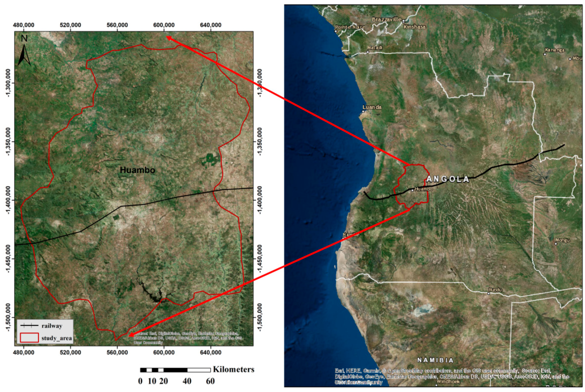
Our study focused on Huambo province within the Central Plateau (12° 29′ 59.99″ S, 15° 39′ 59.99″ E) of Angola (Figure 1). The dominant soils are ferralsols at higher elevations and alluvial fluvisols at lower elevations. With an area of approximately 34,270 km² and a population of approximately 1.9 million inhabitants, Huambo province is divided into 11 municipalities. It is 1700 m a.s.l., with a mean annual temperature of 20 °C, and annual rainfall ranges from 1200 to 1600 mm [47,48,49]. The climate is humid meso-thermal with dry winters and warm summers. Most of the precipitation occurs during the warmer summer months (October to April), with heavy precipitation in December and March. Six major rivers originate in Huambo, many of which drain into the Atlantic Ocean. Vegetation in Huambo province consists largely of four types: highland forests (Afromontane forests), Miombo woodlands, swamps, and dry grasslands [50,51,52]. The landscape is mainly comprised of Miombo forests, which is subdivided into closed and open forests, and, in lower areas, savanna woodlands intercepted by grasslands are more prominent. These vegetation types are difficult to map because they are scattered and patchy. The purpose of mapping the vegetation is to show their spread and distribution across the whole province. Frequent intense fires, tree cutting for charcoal, and clearing for new agricultural fields affect vegetation distributions and structure.

2.2. Ground Data Collection and Processing

We established 18 circular sample plots (radius: 25.2 m) in open and closed Miombo forests by distributing them in a random fashion to represent the major vegetation types in Huambo Province. Prior to sample plot establishment, we used satellite images of land cover to delineate the potential forest area for sampling. When possible, study sites were identified from the images, and we conducted field surveys at the sites to ensure the areas were suitable for sample plot establishment. The locations of the plots are presented in [53]. For each sampled forest patch, the total area of all the plots should comprise at least 2% of the total forest patch area; for example, in a 20-ha forest patch, a total area of 0.4 ha would be sampled. For each sampled tree within a plot, diameter at breast height (DBH) was measured using diameter tape and heights were measured using a hypsometer Vertex IV (Haglof Inc., Långsele, Sweden). Sample plot data allowed us to calculate density (stems·ha⁻¹), basal area (BA; m²·ha⁻¹), and stem volume (m³·ha⁻¹) for grassland, open and closed Miombo. Analysis of sample plot data was conducted using SAS V.9.4 and MATLAB R2017b professional edition (MathWorks©, Inc., Natick, MA, USA). We determined the parameter values of diameter growth functions using regression analysis [54].

2.2.1. Modelling Height–Diameter Relationships

Data for many tree species were rare in our sampling efforts, thus it was not possible to develop a species-specific height–diameter models for several species. Consequently, we pooled the data from all species to develop a height–diameter model applicable to all species. We used a versatile nonlinear growth function, the Näslund function [55], to fit the data. This function has frequently been used to model the height–diameter relationship for several tree species because of its flexibility [56,57,58,59]. The Näslund function is:

$$H_{ij}=1.3+{\left[\frac{DB{H}_{ij}}{\left\{b_1+b_{2}DB{H}_{ij}\right\}}\right]}^3+{\epsilon }_{ij}$$

(1)

where H_ij and DBH_ij are the total height and DBH measurements, respectively, for the jth tree on the ith sample plot, b₁ and b₂ are parameters to be estimated, and ε_ij is an error term. A value of 1.3 m, the height at which DBH was measured, was added to avoid the predictions of zero height when DBH approaches zero.

For modelling categorical variables [29,60], we included two dummy variables (V₁, V₂) to describe the effects of three vegetation types on height–diameter relationship (

Table 1. Representation of matrix calculation.

Vegetation Type	V1	V2
Grassland	0	0
Closed Miombo forest	1	0
Open Miombo forest	0	1

).

The effect was best described when b₁ of the base function (Equation (1)) was expressed as a linear function of dummy variables. The base function was extended through redefining its parameter b₁ as a function of tallest tree per sample plot (H_max, m) and stand basal area (BA, m² ha⁻¹), as they significantly contributed to the height–diameter relationship in this setting. Other stand variables, such as stem number per hectare and quadratic mean diameter per sample plot were also subsequently added to the model. However, no significant improvement in the fit statistics was observed. We used an expanded form of the above function with two dummy variables and two stand-level variables:

$$\begin{gathered} H_{ij}=1.3+{\left[\frac{DB{H}_{ij}}{\left\{\left(b_1+u_{i1}\right)+\left(b_2+u_{i2}\right)DB{H}_{ij}\right\}}\right]}^3{\epsilon }_{ij}+ \\ \mathrm{with}{b}_1={\alpha }_1{V}_1+{\alpha }_2{V}_2+{\alpha }_3{H}_{maxi}^{{\alpha }_4}+{\alpha }_5 B{A}_i \end{gathered}$$

(2)

where H_maxi is the height of the tallest tree on the ith sample plot; ${\alpha }_1$, ${\alpha }_2$, …, ${\alpha }_5$, and b₂ are parameters to be estimated, and V₁ and V₂ are dummy variables that account for the effects of vegetation types. The vectors of errors ε_ij and sample plot-level random effects (u_i1, u_i2) are defined by ${\mathit{\epsilon }}_{\mathit{i}}~\mathit{N}\left(\mathbf{0}, \mathit{R}\right)$ and ${\mathit{u}}_{\mathit{i}}~\mathit{N}\left(\mathbf{0}, \mathit{D}\right)$, respectively, meaning that vectors ε_i and u_i were assumed to have normal distributions with zero mean and within-sample plot variance–covariance matrices R and D, respectively [61,62]. The height–diameter model (Equation (2)) was estimated using the mixed modelling method.

2.2.2. Modelling Stem Volumes of Miombo Forest Species

We selected an exponential function to most effectively describe the stem volume variations. We modelled stem volume using DBH and total height (HEIGHT) as the main predictors and vegetation types, stand basal area, and DBH-to-quadratic mean diameter ratio (dq) were used as covariate predictors:

$$\begin{gathered} S{V}_{ij}=b_{1}exp\left(b_{2}DB{H}_{ij}^2\times HEIGH{T}_{ij} \right)+{\epsilon }_{ij} \\ \mathrm{with} b_1={\alpha }_1{V}_1+{\alpha }_2{V}_2+{\alpha }_{3}B{A}_i+{\alpha }_4 d{q}_{ij} \end{gathered}$$

(3)

where SV_ij is the stem volume of the jth tree on the ith sample plot; ${\alpha }_1$, ${\alpha }_2$, …, ${\alpha }_4$, and b₂ are parameters to be estimated, V₁ and V₂ are dummy variables that account for the effects of vegetation types on the stem volume, and ${\epsilon }_{ij}$ is an error term that is assumed to be normally distributed with mean zero and constant variance. The volume model was estimated using the nonlinear ordinary least squares regression method.

2.3. Remotely Sensed Data and Application

To derive deforestation patterns in Miombo forests, we used Landsat imagery from two different sensors, the Landsat-8 Operational Land Imager (OLI; 2013–2016) and the Landsat-7 Enhanced Thematic Mapper Plus (ETM+; 1999–2016), for the study period from 2000 (August) to 2017 (August). All products were obtained through the United States Geological Survey (USGS) Earth Explorer (EE) tool.

2.3.1. Pre-Processing of Remotely Sensed Data

Due to the size of the study area, we used five frames from Landsat-7 and four frames from Landsat-8, combined the bands (

Table 2. Landsat satellite sensor characteristics.

Landsat 8
Band	Wavelength	Application	Resolution (m)
Band 2—Blue	0.452–0.512	Bathymetric mapping, distinguishes soil from vegetation and deciduous from coniferous vegetation	15
Band3—Green	0.533–0.590	Emphasizes peak vegetation, which is useful for assessing plant vigor	15
Band 4—Red	0.636–0.673	Discriminates between vegetation slopes	15
Band 5—Near Infrared (NIR)	0.851–0.879	Emphasizes biomass content and shorelines	15
Landsat 7
Band 1—Blue	0.45–0.52	Bathymetric mapping, distinguishes soil from vegetation and deciduous from coniferous vegetation	30
Band2—Green	0.52–0.60	Emphasizes peak vegetation, which is useful for assessing plant vigor	30
Band 3—Red	0.63–0.69	Discriminates between vegetation slopes	30
Band 4—Near Infrared (NIR)	0.77–0.90	Emphasizes biomass content and shorelines	30

Source: [63].

) for each data frame, and eliminated the null values using the Copy Raster toolset in ArcGIS desktop V.10.5.1 (ESRI Inc., Redlands, CA, USA). Finally, we mosaiced the frames for each year separately using the Mosaic to New Raster tool.

To improve the image quality and eliminate sources of errors, we used the Fast Line-of-sight Atmospheric Analysis of Hypercubes (FLAASH) method, a radiometric correction method, in the Environment for Visualizing Images V.5.1 software (ENVI; Harris Geospatial Solutions, Boulder, CO, USA). We confirmed the results by examining the histogram values produced from the FLAASH procedure. To georeference the images, we used the defined nominal Landsat satellite track (path and row) approach, where the nearest World Reference System (WRS) path and row to the line of sight was the scene’s center; the whole process was conducted using the USGS website. In addition, we resampled the image from 2000 from a 15 m spatial resolution to 30 m using the nearest neighbor method. We did this to equalize the cell sizes in either the images of 2000 or 2017. The study of land use classification in Angola is very limited, unfortunately, due to lack of quality satellite information, and for this study area we took maximum advantage of existing spectral sources. Although using different Landsat imagery can cause errors, there are some pre-processing steps that can help users to reduce the errors as much as possible. In this case, we used the value histogram of the same objects in different images to make sure the differences between the digital number DN values were because of land cover changes during the time, not the nature of the image. For example, by comparing dark and artificial objects that did not change during the time (or for which changes were not significant), we were able to verify the accuracy of our methodology.

2.3.2. Data Processing

For the classification process, we separated the work into three stages. First, we decided to base the land use classification on four different classes (vegetation areas, urban areas, water bodies, and others). We then identified certain areas of pixels (training areas) for each class using polygons, and we extracted a signature file from the training samples to supervise the classification process (

Table 3. Training data used in supervised classification process.

Classes	Pixels	Area (km2)	Percentage
Vegetation area	5,598,267	503,844.03	15
Urban area	2,827,356	254,462.04	7.57
Water	2,349,593	211,463.37	6.29
Other land-cover	1,516,868	136518.12	4.06
Total	12,292,084	1,106,287.56	32.92

). A maximum likelihood classifier was used to classify the study area into the desired classes. Finally, the percentage of area in each class was calculated for 2000 and 2017. The spatial-temporal variability of normalized difference vegetation index NDVI was assessed to study deforestation using harmonic analysis. We first spatially normalized observations to reduce seasonality. Subsequently, we detected deforestation by assessing whether a newly acquired observation (satellite image) in the monitoring period is in an extreme change when compared against spatially normalized values in present time data defined over a reference period. The calculation of the NDVI for multi-date satellite images of Landsat (7, 8) was used to perform change detection of the deforestation in Huambo Miombo. The differences between the percentages of each class (2000–2017) were used as a basis for further analyses. The NDVI, as one of the most successfully used vegetation spectral indices, allows comparison between inter-annual and seasonal changes in vegetation. The NDVI measures the amount of green vegetation in an area and is used to distinguish forested from deforested areas. Also, to investigate the impact of railway constriction on deforestation and land-cover change, we compared the land-cover type using a buffer zone with radius of 5 km around the “Caminho de ferro de Benguela” Benguela railway.

2.3.3. Assessing the Management Zones in Miombo Forests

Using the watershed areas and land cover of the study area, we devised a method to delineate management zones (MZ). First, topographic attributes were calculated from elevation data using TAPES (Terrain Analysis Programs for the Environmental Sciences), a useful program designed to handle the complexity of individual landscape processes and patterns encountered in delineating the appropriate spatial and temporal scales [64].

We then removed imperfections or sinks of the digital elevation model (DEM) with the fill tool in the ArcGIS spatial analyst toolbox. Fill layer was used to calculate the hydrologic flow direction layer using the direction toolset in the spatial analyst toolbox, hydrology. The hydrologic flow direction raster was analysed as an input of the basin layer to find all sets of connected pixels that belong to the same drainage basin. Basin tool was used to create a raster delineating all drainage basins, hereafter referred to as watersheds. A watershed is the upslope area that contributes flow to a common outlet as concentrated drainage. After transforming the results of the basin tool to a vector polygon based on visual assessment of land cover type, we specified a MZ for each watershed area. Finally, for simplicity in calculating the percentage of each MZ, we merged similar MZs together.

3. Results

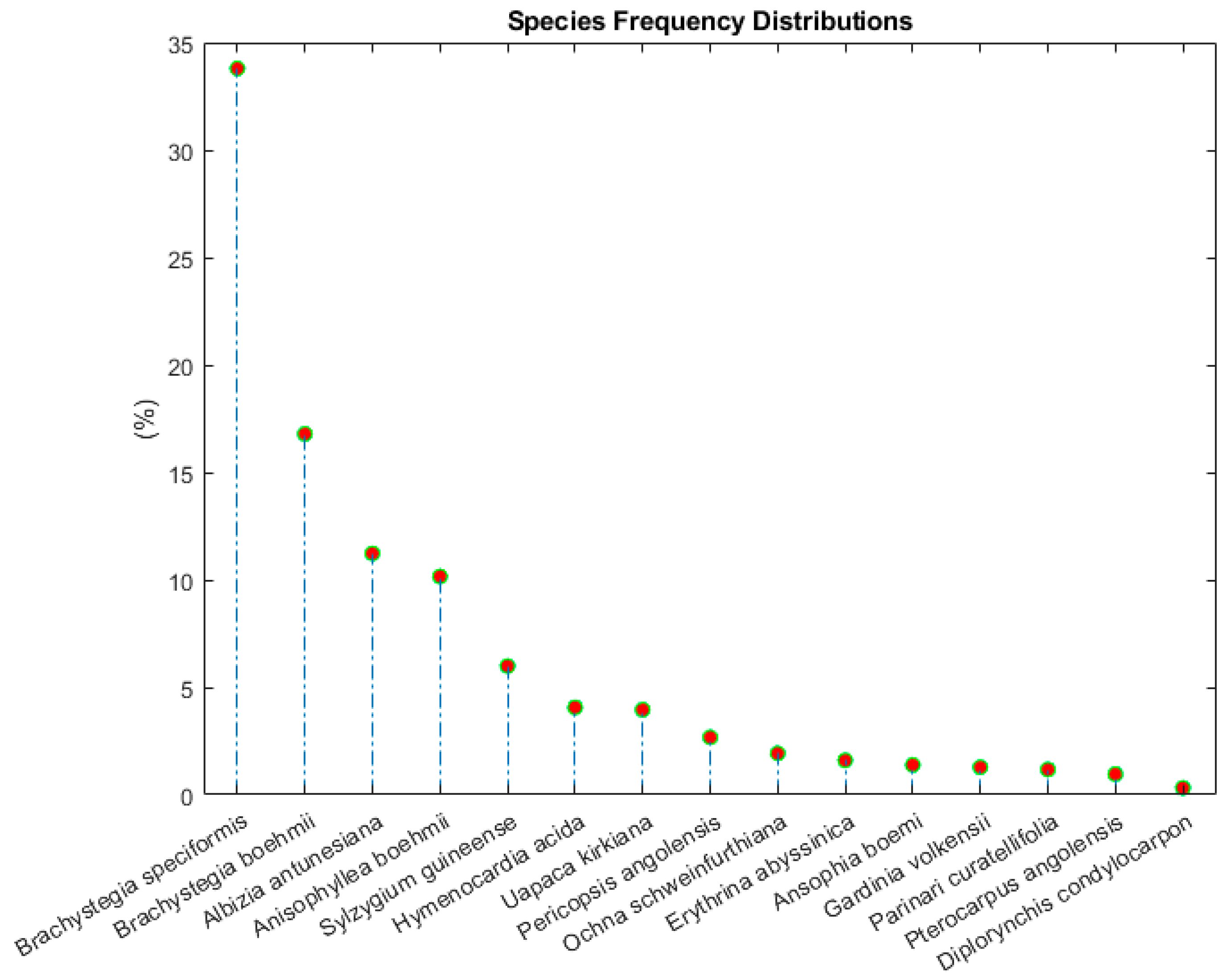
Most of the 934 trees sampled were less than 9 m height with a mean DBH of 12.4 cm and the mean basal area per ha was 0.87 m². Comparatively, trees were shorter in grassland (height of 2.8 m with mean DBH of 4.9 cm) and open Miombo forest vegetation type with 5.3 m in height and mean DBH 8.2 cm. In closed Miombo, trees were of 30 cm DBH. The number of recorded tree species in the study area were 15, and the frequency distribution of the species is summarized in Figure 2. Four tree species predominate in Huambo Miombo (Brahcystegia spiciformis, Brachystegia boehmii, Anysophyllea boehmii and Albizia antunesiana).

3.1. Height–Diameter Relationships

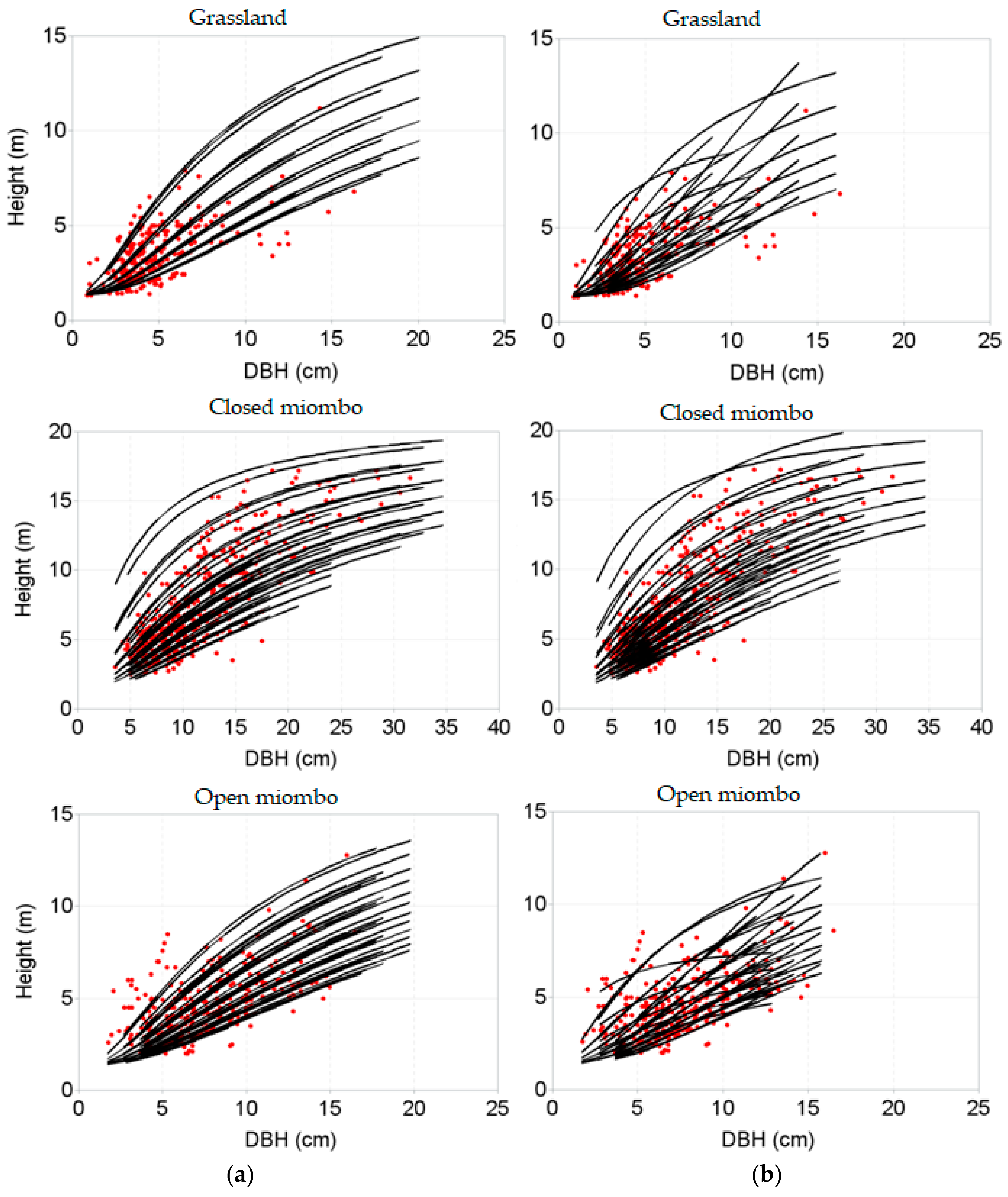
The mixed-effects model described a large proportion of the total variations in the height–diameter relationships without significant residual trends; all parameter estimates were significant (p < 0.05) (

Table 4. Parameter estimates, variance components, and fit statistics of the mixed effects model (Equation 2). AIC: Akaike’s information criterion; BIC: Schwarz’s information criterion; α₁, …, α₅, b₂: fixed parameters; u_i1, u_i2 = random effect parameters; σ²_ui1: variance of u_i1; σ²_ui2: variance of u_i2; σ²: residual variance.

Components	Parameter Estimates	Standard Errors	t-Value	p-Value
${\mathit{\alpha }}_{\mathbf{1}}$	0.671541	0.1076	6.24	<0.0001
${\mathit{\alpha }}_{\mathbf{2}}$	0.476616	0.0861	5.53	<0.0001
${\mathit{\alpha }}_{\mathbf{3}}$	1.922154	0.1961	9.80	<0.0001
${\mathit{\alpha }}_{\mathbf{4}}$	0.069407	0.0156	4.46	0.0456
${\mathit{\alpha }}_{\mathbf{5}}$	−0.19517	0.0180	−10.84	<0.0001
${\mathit{b}}_{\mathbf{2}}$	0.366381	0.00514	71.31	<0.0001
Variance		Fit statistics
σ2ui1	2.0149	R2	0.84
σui1ui2	−0.1821	AIC	3366
σ2ui2	0.01662	BIC	3370
σ2	0.4418

). Including the sample plot-level random effects in the model significantly increased the fit with reference to the model fitted without random effects; the R² value increased by 14% in comparison to the ordinary least squares model. Sample plot-specific height–diameter curves simulated using only the fixed portion of the mixed model (mean model) and mixed-effects model (both fixed and random portions included) seemed different. The latter curves passed through the middle of the data for each plot, which indicated that calibration using the height measurement of at least one randomly selected tree worked well for the sample plot-specific model.

The selected model (Näslund function) is based on the growth theory (faster increase of height in earlier stages and slower increase in later stages) [56,65]. Näslund function fitted best to our data due to its flexibility in fitting height–diameter relationships for a number of tree species (Figure 3) [58].

3.2. Volume Assessment

The exponential function described a large proportion of the stem volume variations [R² = 0.846; RMSE = 0.0276 (m³ ha⁻¹); AIC = 4106] without significant residual trends, and all parameter estimates were highly significant (p < 0.0001;

Table 5. Parameter estimates and fit statistics of the volume model (Equation 3).

Parameter	Estimate	Standard Error	t-Value	p-Value
${\mathit{\alpha }}_{\mathbf{1}}$	−0.011190	0.002550	−4.39	<0.0001
${\mathit{\alpha }}_{\mathbf{2}}$	−0.018250	0.003920	−4.65	<0.0001
${\mathit{\alpha }}_{\mathbf{3}}$	0.006604	0.000358	18.47	<0.0001
${\mathit{\alpha }}_{\mathbf{4}}$	0.021572	0.000566	38.14	<0.0001
${\mathit{b}}_{\mathbf{2}}$	0.000144	9.837 × 10−7	146.61	<0.0001

).

The vegetation type-specific model behaved significantly differently for different vegetation types, which suggested that vegetation types could also affect stem volumes (Figure 4).

3.3. Deforestation Patterns

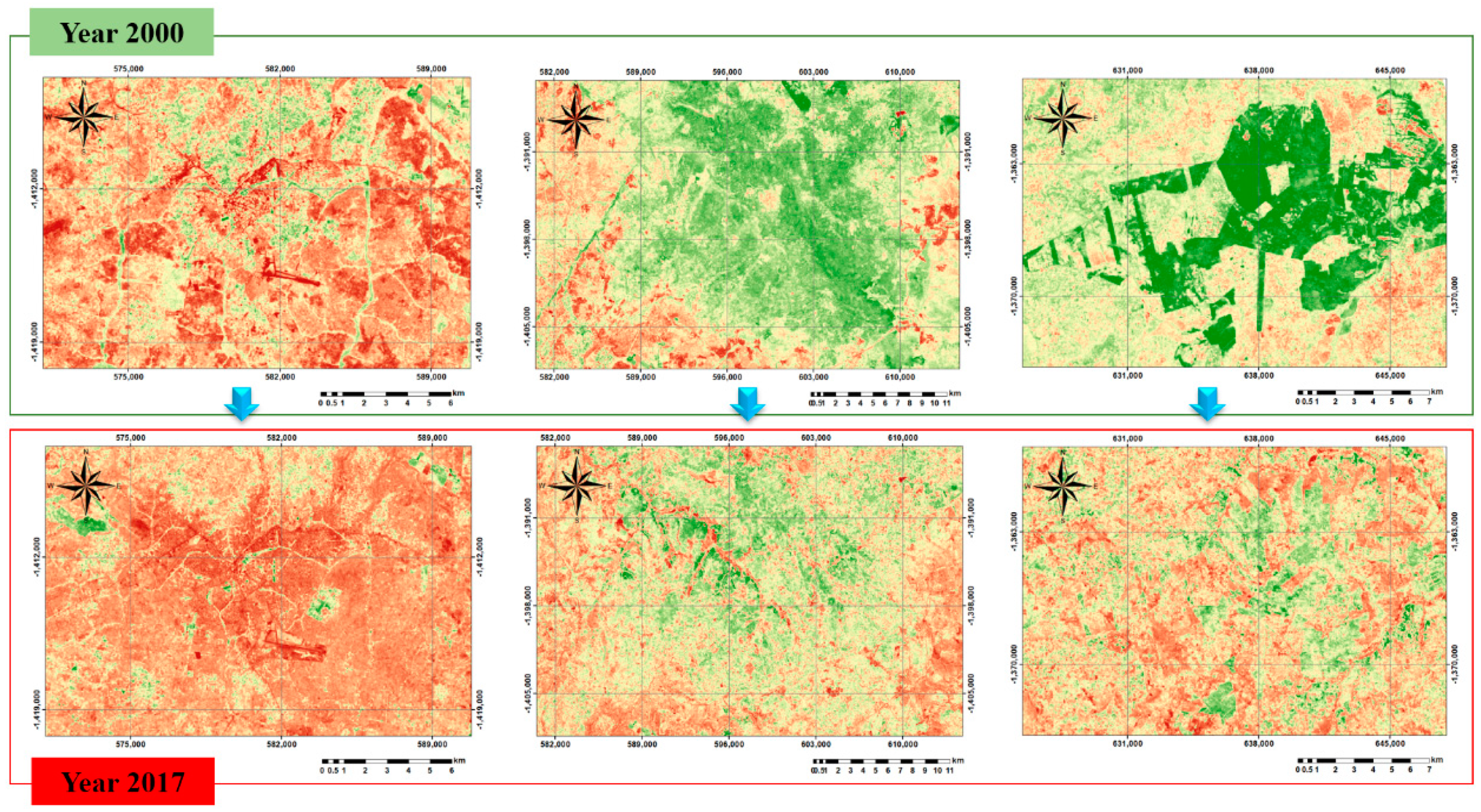
The loss of natural vegetation and plantation is the most visible evidence of deforestation pattern in Huambo. The main argument for this assertion is the ongoing vegetation loss (17% from 2000 to 2017) and agricultural expansion (confirmed by other studies) which is also verified by the remote sensing analysis (

Table 6. The percentages of land use (LU) and land cover (LC) changes from 2000 to 2017 for the entire study area. The value for other land cover is quite large and represents bare land and agriculture land together.

	Year 2000		Year 2017
	Area (km2)	Percentage (%)	Area (km2)	Percentage (%)
Vegetation area	1,953,854.73	58.16	1,384,050.96	41.20
Urban area	338,998.59	10.10	702,008.91	20.90
Water	12,616.29	0.37	4889.61	0.14
Other land cover	1,054,063.53	31.37	1,268,583.66	37.76

and

Table 7. The percentages of LU/LC changes for the “Caminho de ferro de Benguela” Benguela railway line (Figure 1).

	Year 2000		Year 2017
	Area (km2)	Percentage (%)	Area (km2)	Percentage (%)
Vegetation area	99,166.4	59.9	46,332.3	28.0
Urban area	25,349.4	15.3	40,370.6	24.4
Water	109.9	0.07	40.9	0.02
Other land cover	40,819.6	24.7	78,701.6	47.6

). This pattern was accentuated along the railway line (Caminho de ferro de Benguela) where natural forest was exploited to supply wood for the steam locomotives. Figure 5 of forested areas in Angola in 2000 and 2017 shows that many forests have suffered from deforestation. From our detailed analysis of the LC map, the impact is devastating and natural forests in Huambo appear to not be managed at all.

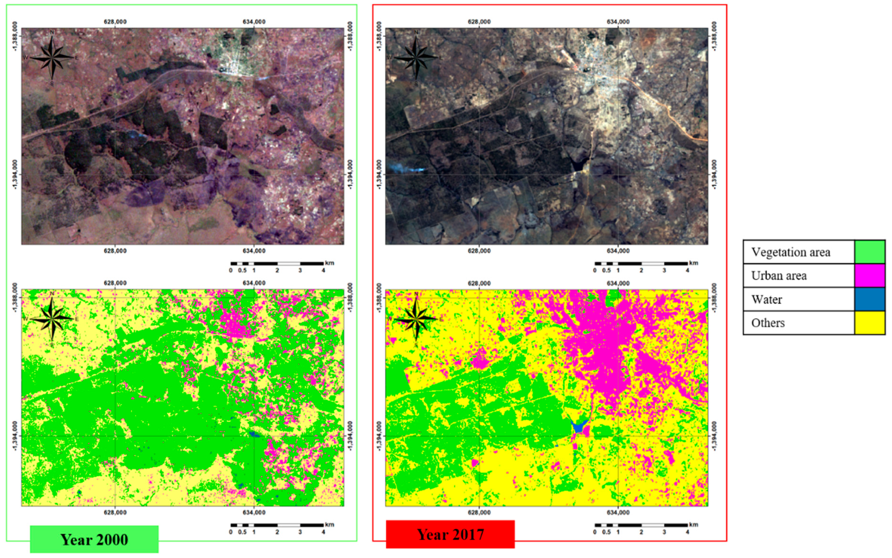
The change of forest cover is evident in Figure 6 where the most patterns are shown in conversion of natural forest to agriculture land and disappearance of forest plantation (Figure 6). This is a result of the logging and slash-and-burn agriculture of subsistence, where farmers typically plant their crops, deplete the soil, and move on after a couple of years. Figure 7 shows an area which remained unchanged between 2000 and 2017.

3.4. Delineated Management Zones

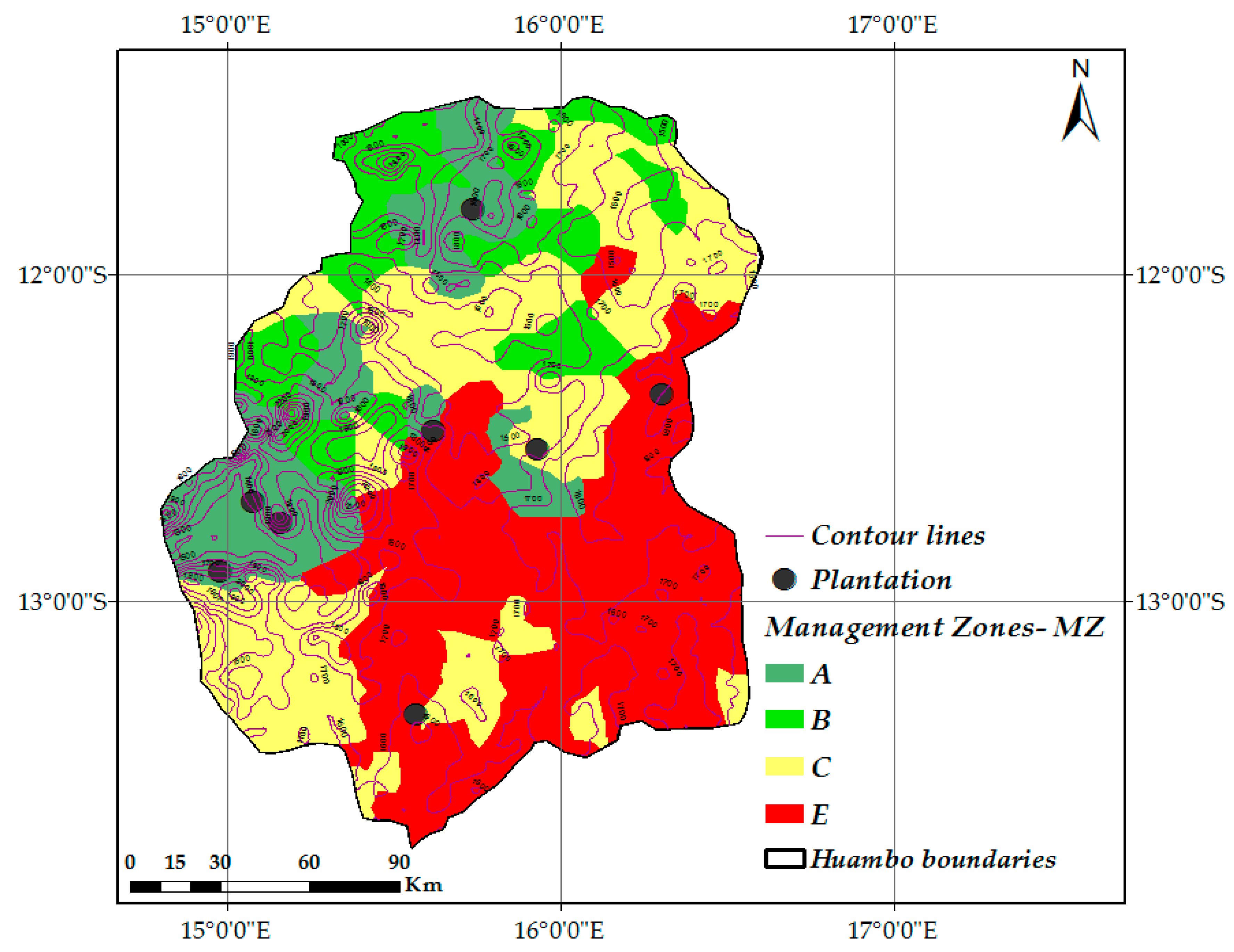
Four management zones (MZ) were aligned with elevation attributes of the landscape, whereby MZ–A and MZ–B represent lower elevations in the north-western portion of the study area (Figure 8). MZ–E comprises upland areas (from 1484 m to 1897 m) in the southern portion of the study area; MZ–C can be interpreted as a combination of elevation areas from 1275 m to 1609 m above sea level (Figure 8). For a thorough description of the management zones, see [54]. Vegetation types also differ in each management zone, whereby MZ–E represents agricultural land and bare soil, MZ–C consists of grasslands or savannas that include MZ-D, as described in [54], MZ–B contains open Miombo forests, and MZ–A is comprised of closed Miombo forests. It was not possible to represent the plantations by a single management zone because they were found distributed across other zones with similar elevation patterns.

4. Discussion

4.1. Tree Height–Diameter Model and Description of the Management Zones

Tree height and DBH are important variables in forest inventories and timber management as these variables are necessary for estimating stand volume and biomass. Tree height data modelled from DBH can be employed as an input variable in various forest models, together with DBH, such as growth and yield models, site productivity models, crown models, biomass models, and carbon budget models [61]. These models serve as important tools in forest management decision-making. Realistic description of stand growth and stem volume, and simulation of stand structure and dynamics, is possible only with use of the stand-specific height–diameter models [66]. The height–diameter models may be used to evaluate site productivity [36,45,67,68]. Developing precise stand-specific height–diameter models is considered one of the most important tasks in forest planning, inventory design, and monitoring of stand dynamics [56]. Precise height–diameter models developed with subject-specific (e.g., sample plot-specific) variations are included in the model [57,59,66]. The presented sample plot-specific mixed effects height–diameter model can be used for characterization of the vertical stand structures, estimation of volume and biomass, and simulation of stand dynamics for each vegetation zone of the studied forest.

The major challenge in our study is that a large number of tree species existed with relatively few observations for the majority [69]. The task of developing a species-specific height–diameter model for several species seems intractable, at least initially, and the mixed species approach used is advantageous when the species is treated as a random effect to circumvent the need for grouping the data [70]. However, we did not consider this because of computational complexity, but species-specific effects on the height–diameter relationships were included using the dummy variable modelling approach. This approach is considered suitable for modelling height–diameter relationships using the data originated from multi-layered and multi-species stands [57,71,72]. We chose the best functional form (Näslund function) to adequately describe the variations in the height–diameter relationship of individual trees for each vegetation type (Figure 3). Näslund function is based on the growth theory (faster increase of height in earlier stages and slower increase in the later stages) [56,61,65,73] and is best suited to our data due to its pronounced flexibility for fitting data acquired from multiple tree species [58,59]. By looking at the growth curve patterns, we hoped to discover some similar patterns or principles that govern the growth of the species in the respective vegetation types. The height–diameter model is significantly different for each vegetation type, which indicates that the vegetation types significantly influence height–diameter relationships (Figure 3). The grassland zone was found inside MZ–E (1,484 m to 1897 m a.s.l.), which is the most heavily deforested area, followed by open Miombo forests of MZ–C and MZ–B (Figure 8).

4.2. Deforestation Patterns of Miombo Forests in Huambo Province

One of the objectives of the study was to identify deforestation patterns and assess important management criteria in degraded Miombo forest areas. By analysing spatial and temporal information from maps, satellite data and field observations, it was possible to map, quantify, analyze and explain the natural and human influences on the landscape over time. The landscape patterns represent the key to studying correlation between woodland vegetation and landforms. It provided the opportunity to focus on issues related to vegetation variability, forest zoning and forest fragmentation.

From a historical perspective, deforestation in Angola accelerated after the civil war and not during the colonial era. Many believe that with the arrival of the Portuguese in Angola, intensive exploitation of forest resources began due to the high timber demands for ships at that time. Large quantities of precious timber were exported to Portugal [74], and timber was needed to supply steam trains on the Benguela railway (Caminho de ferro de Benguela), both of which increased pressure on forests. Over time, natural forests were unable to recover and regrow, thus many turned to new introduced species, such as Eucalyptus spp), Thuja spp., Pinus spp. and Grevillea robusta, which were planted in very large areas along the railway [48,75]. Within five kilometers of the railway, deforestation was particularly evident between 2000 and 2017 (Table 6). Local populations use the plantations for firewood. The eucalypts plantations alongside the Benguela Railway in Huambo are some of the largest in all of Africa [76]; they were originally planted to provide firewood for the steam locomotives. The plantations were quickly deforested, although natural regeneration can help forest growth and recovery (Figure 6 and Figure 7). In some areas with poor access, some plantations were largely untouched and conserved (Figure 8). Most of the plantations belong to private enterprises (mainly the railway and pulp companies), while the remaining plantations are state property managed by the Ministry of Agriculture and Rural Development.

During the Angolan civil war, large portions of the population relocated to the cities for security reasons; however, with the Luena Peace Agreement in April 2002 [77] and the end of the civil war, millions of people were forced to leave the cities and return to their homes, and this initiated a period of rapid expansion of agricultural fields. In addition, trees were rapidly harvested by the returning populations who needed firewood for cooking and heating (Figure 5).

From 2000 to 2017, approximately 17% of forest vegetation was lost (Figure 5 and Figure 6; Table 5). The decreased areas of vegetation and the increase of urban areas illustrate the primary changes in vegetation cover throughout the entire study area. Within a radius of 30 to 50 km around Huambo Province, many areas appear to be savanna-like because they contain only a few scattered trees. The expansion of degraded areas initiated near urban areas, and those patterns were accentuated in the south-western and north-eastern portions of the province (Figure 5); many of the areas lost were grasslands or savannas.

From a global perspective, managed forests increase over time, which is largely a result of forest management planning [78,79]. In Angola, however, forested area has decreased over time, which may be explained by the lack of forest management plans and intensive charcoal and firewood production for cooking and heating, as suggested by several other studies [27,42,78]. Schneibel et al suggested that the expansion of agricultural land was a primary contributor to deforestation rates, and they concluded that even during the conflict period and the post-ceasefire period (2002), the expansion of agriculture land was not reduced [42].

Evidence of deforested areas is well documented in Angola, however, no management actions have been described or assessed for these degraded areas. Romeiras et al documented the biogeographic patterns of timber species, and determined that Angolan timber species are under increasing risk [23]; they recommended conservation and sustainable management measures be developed to ensure future forests. Our results addressed this need through the creation of management zones. This creation of management zones is an important first step for future forest planning and highlighting management suggestions considering the current policies in the country. In the absence of baseline information on which to base assessments of rates of deforestation, multi-temporal analysis of remote sensed data seems to be the most readily available option.

The forest management zoning system presented in our article is based on topographic attributes and is linked to the management zones proposed by [54]. The zones can help in the sustainable management of native forests in meeting current and future community needs. The zones are easily distinguishable in the map, as they largely follow the topography of the area.

We recommend that each management zone should be examined to determine the appropriate operations and long-term strategies to ensure that these needs are met. For example, in MZ–E, a predominantly agricultural area, grassland and savanna vegetation consists of shorter trees and a mean DBH of 4.9 cm. In MZ–E, management objectives should seek to maximize the protection of cleared (non-forested) areas and forbid all activities that require complete vegetation removal (e.g., timber harvest, removal of forest products, grazing by domestic stock) to allow forests to regenerate naturally, or even artificially in certain areas. For MZ–C, the objective should be to conserve forest ecosystems while also allowing some production activities, however, with limited tree removal. For MZ–A and B, they could be reserved for the management of native forests for the production of timber, charcoal, and firewood production utilizing the full range of silviculture options, as described in [54]. Conservation should address the environmental values that are dependent on the forest structure. Moreover, activities such as grazing and timber supply, for lease fencing and firewood, respectively, should be allowed only on MZ–B. To determine final forest management zoning in MZ–A and MZ–B, more field investigations and data collection are recommended. Plantation zones should be managed to maximize sustainable timber production based on reliable estimates of annual allowable harvest. However, more studies are needed to adequately evaluate the present state of Angolan forest plantations.

Since growth models (diameter and height growth models), height–diameter models, site productivity models, and stem volume models are important tools for decision-making in sustainable forest management planning, they were considered in this study. However, growth models and site productivity models (dominant height–age models) were not able to be developed due to lack of time series data (repeatedly measured data). The land cover assessment helped in developing management zones where, possibly in the future, we will be able to do this when we collect data from the same sample plots. All these models help determine the annual increment and allowable harvest in every year from any forest, and therefore our height–diameter models and volume models will be helpful in formulating better management plans for Miombo forests.

5. Conclusions

The primary focus of this study was to define patterns of deforestation and propose a management framework for the degraded areas based on our intensive characterization of the forest attributes, including the use of basic height–diameter models. The expansion of agricultural land has been the primary driver of deforestation. The conclusion is that even during the conflict period and afterward, the deforestation rate never decreased. In all cases, informed creation of management zones that are consistent over time and transparent for the purposes of systematic monitoring is critical to the success of sustainable forestry in Angola. Assessments of forest degradation using high-resolution imagery can be useful to map tree cover loss in support of this goal.

Based on our results (Figure 5 and Figure 6), it appears that it is not simply the number of trees removed that threatens the stability of Miombo forests, but also the patterns of deforestation associated with the demand for new agricultural lands and charcoal and firewood production for cooking and heating. The results demonstrate that deforestation is a serious environmental problem in Angola, where the ongoing vegetation loss (17% from year 2000 to 2017), including woodland forest, in the past few decades is accentuated. However, the use of remote-sensing technology in land use classification in Angola is limited, particularly in forest or deforestation change analysis.

The four management zones are distinguishable on the map and growth height–diameter models developed represent a fundamental tool for future studies on forest planning for Miombo forests in Huambo Province, Angola. Using a combination of LC and LU data with topographic data, we concluded that certain types of changes are influenced by terrain morphology.

References

1. Kaplan, J.O.; Krumhardt, K.M.; Zimmermann, N. The prehistoric and preindustrial deforestation of Europe. Quat. Sci. Rev. 2009, 28, 3016–3034. [Google Scholar] [CrossRef]
2. IUCN. Deforestation and Forest Degradation; IUCN: Gland, Switzerland, 2017. [Google Scholar]
3. FAO. Assessing Forest Degradation Assessing Forest Degradation; Food and Agriculture Organization of the United Nations: Rome, Italy, 2011. [Google Scholar]
4. Geist, H.; Lambin, E.F. Proximate Causes and Underlying Driving Forces of Tropical Deforestation. Bioscience 2002, 52, 143–150. [Google Scholar] [CrossRef]
5. Defries, R.S.; Rudel, T.; Uriarte, M.; Hansen, M. Deforestation driven by urban population growth and agricultural trade in the twenty-first century. Nat. Geosci. 2010, 3, 178–181. [Google Scholar] [CrossRef]
6. Kissinger, G.; Herold, M.; De, V.; Angelsen, A.; Bietta, F.; Bodganski, A.; Boucher, D.; Boyle, T.; Brickell, E.; Defries, R.; et al. Drivers of Deforestation and Forest Degradation. CIFOR Occas. Pap. 2012. [Google Scholar] [CrossRef]
7. Ryan, C.M.; Hill, T.; Woollen, E.; Ghee, C.; Mitchard, E.; Cassells, G.; Grace, J.; Woodhouse, I.H.; Williams, M. Quantifying small-scale deforestation and forest degradation in African woodlands using radar imagery. Glob. Chang. Biol. 2012, 18, 243–257. [Google Scholar] [CrossRef]
8. Schielein, J.; Börner, J. Recent transformations of land-use and land-cover dynamics across different deforestation frontiers in the Brazilian Amazon. Land Use Policy 2018, 76, 81–94. [Google Scholar] [CrossRef]
9. Rosa, I.M.D.; Smith, M.J.; Wearn, O.R.; Purves, D.; Ewers, R.M. The Environmental Legacy of Modern Tropical Deforestation. Curr. Biol. 2016, 26, 2161–2166. [Google Scholar] [CrossRef] [Green Version]
10. Vieilledent, G.; Grinand, C.; Rakotomalala, F.A.; Ranaivosoa, R.; Rakotoarijaona, J.R.; Allnutt, T.F.; Achard, F. Combining global tree cover loss data with historical national forest cover maps to look at six decades of deforestation and forest fragmentation in Madagascar. Biol. Conserv. 2018, 222, 189–197. [Google Scholar] [CrossRef]
11. Krishna, V.V.; Kubitza, C.; Pascual, U.; Qaim, M. Land markets, Property rights, and Deforestation: Insights from Indonesia. World Dev. 2017, 99, 335–349. [Google Scholar] [CrossRef]
12. Hoffmann, C.; García Márquez, J.R.; Krueger, T. A local perspective on drivers and measures to slow deforestation in the Andean-Amazonian foothills of Colombia. Land Use Policy 2018, 77, 379–391. [Google Scholar] [CrossRef]
13. Greenpeece Tackling Deforestation and Forest Degradation: A Case for EU Action in 2017. 2017. Available online: https://fern.org/NGOcallforaction (accessed on 17 October 2018).
14. Norris, K. Ecology: The Tropical Deforestation Debt. Curr. Biol. 2016, 26, R770–R772. [Google Scholar] [CrossRef] [PubMed]
15. Strömquist, L.; Ingvar, B. Strömquist_Backéus_2009_Integrated landscape analyses of change of miombo woodland in Tanzania and its implication for environment and human livelihood. Geogr. Ann. 2009, 1, 31–45. [Google Scholar] [CrossRef]
16. Scherr, S.; Shames, S.; Friedman, R. Defining Integrated Landscape Management for Policy Makers; EcoAgriculture: Washington, DC, USA, 2013. [Google Scholar]
17. Jansen, L.J.M.; Bagnoli, M.; Focacci, M. Analysis of land-cover/use change dynamics in Manica Province in Mozambique in a period of transition (1990-2004). For. Ecol. Manage. 2008, 254, 308–326. [Google Scholar] [CrossRef]
18. Kleemann, J.; Baysal, G.; Bulley, H.N.N.; Fürst, C. Assessing driving forces of land use and land cover change by a mixed-method approach in north-eastern Ghana, West Africa. J. Environ. Manage. 2017, 196, 411–442. [Google Scholar] [CrossRef] [PubMed]
19. Brun, C.; Cook, A.R.; Lee, J.S.H.; Wich, S.A.; Koh, L.P.; Carrasco, L.R. Analysis of deforestation and protected area effectiveness in Indonesia: A comparison of Bayesian spatial models. Glob. Environ. Chang. 2015, 31, 285–295. [Google Scholar] [CrossRef]
20. Prins, E.; Kikula, I.S. Deforestation and regrowth phenology in miombo woodland - Assessed by Landsat Multispectral Scanner System data. For. Ecol. Manage. 1996, 84, 263–266. [Google Scholar] [CrossRef]
21. Jansen, L.J.M.; Carrai, G.; Morandini, L.; Cerutti, P.O.; Spisni, A. Analysis of the spatio-temporal and semantic aspects of land-cover/use change dynamics 1991-2001 in Albania at national and district levels. Environ. Monit. Assess. 2006, 119, 107–136. [Google Scholar] [CrossRef]
22. USAID. Biodiversity and Tropical Forest Assessment for Angola. Available online: http://www.usaidgems.org/Documents/FAA&Regs/FAA118119/Angola2013.pdf (accessed on 20 October 2018).
23. Romeiras, M.M.; Figueira, R.; Duarte, M.C.; Beja, P.; Darbyshire, I. Documenting biogeographical patterns of African timber species using herbarium records: A conservation perspective based on native trees from Angola. PLoS One 2014, 9. [Google Scholar] [CrossRef]
24. Blaser, J.; Sarre, A.; Poore, D.; Johnson, S. Status of Tropical Forest Management 2011; ITTO Technical Series; International Tropical Timber Organization: Yokohama, Japan, 2011; Vol. 38, ISBN 4902045788. [Google Scholar]
25. Hansen, M.C.; Potapov, P.V.; Moore, R.; Hancher, M.; Turubanova, S.A.; Tyukavina, A.; Thau, D.; Stehman, S.V.; Goetz, S.J.; Loveland, T.R.; et al. High-resolution global maps of 21st-century forest cover change. Science 2013, 342, 850–853. [Google Scholar] [CrossRef]
26. FAO. Angola: Country Report To the International Conference and Programme. Available online: http://www.fao.org/fileadmin/templates/agphome/documents/PGR/SoW1/africa/ANGOLA.pdf (accessed on 23 April 2018).
27. Schneibel, A.; Frantz, D.; Röder, A.; Stellmes, M.; Fischer, K.; Hill, J. Using annual landsat time series for the detection of dry forest degradation processes in south-central Angola. Remote Sens. 2017, 9. [Google Scholar] [CrossRef]
28. Koirala, A.; Kizha, A.R.; Baral, S. Modeling Height-Diameter Relationship and Volume of Teak ( Tectona grandis L. F.) in Central Lowlands of Nepal. J. Tropic. For. Environ. 2017, 28–42. [Google Scholar] [CrossRef]
29. Sharma, R.P.; Brunner, A.; Eid, T. Site index prediction from site and climate variables for Norway spruce and Scots pine in Norway. Scand. J. For. Res. 2012, 27, 619–636. [Google Scholar] [CrossRef]
30. Li, Y.Q.; Deng, X.W.; Huang, Z.H.; Xiang, W.H.; Yan, W.D.; Lei, P.F.; Zhou, X.L.; Peng, C.H. Development and evaluation of models for the relationship between tree height and diameter at breast height for Chinese-fir plantations in subtropical China. PLoS One 2015, 10, 1–21. [Google Scholar] [CrossRef] [PubMed]
31. Cutini, A.; Chianucci, F.; Manetti, M.C. Allometric relationships for volume and biomass for stone pine (Pinus pinea L.) in Italian coastal stands. IForest 2013, 6. [Google Scholar] [CrossRef]
32. Liu, M.; Feng, Z.; Zhang, Z.; Ma, C.; Wang, M.; Lian, B.; Sun, R.; Zhang, L. Development and evaluation of height diameter at breast models for native Chinese Metasequoia. PLoS One 2017, 12, 1–16. [Google Scholar] [CrossRef]
33. Osman, E.M.H.; Idris, E.Z.A.; Ibrahim, E.M.M. Height-Diameter Prediction Models for Some Utilitarian Natural Tree Species. JFPI 2013, 2, 31–39. [Google Scholar]
34. Mugasha, W.A.; Bollandsås, O.M.; Eid, T. Relationships between diameter and height of trees in natural tropical forest in Tanzania. South. For. 2013, 75, 221–237. [Google Scholar] [CrossRef]
35. Husch, B.; Beers, T.W.; Kershaw, J.A.K., Jr. Forest Mensuration, 4th ed.; John Wiley & Sons: Hoboken, NJ, USA, 2002. [Google Scholar]
36. Duan, G.; Gao, Z.; Wang, Q.; Fu, L. Comparison of Different Height – Diameter Modelling Techniques for Prediction of Site Productivity in Natural Uneven-Aged Pure Stands. Forests 2018, 9, 63. [Google Scholar] [CrossRef]
37. Trorey, L.G. A Mathematical method for the construction of diameter height curves based on site. For. Chron. 1932, 8, 121–132. [Google Scholar] [CrossRef]
38. Aishan, T.; Halik, Ü.; Betz, F.; Tiyip, T.; Ding, J.; Nuermaimaiti, Y. Stand structure and height-diameter relationship of a degraded Populus euphratica forest in the lower reaches of the Tarim River, Northwest China. J. Arid Land 2015, 7, 544–554. [Google Scholar] [CrossRef]
39. Wang, X.; Yu, D.; Wang, S.; Lewis, B.J.; Zhou, W.; Zhou, L.; Dai, L.; Lei, J.; Li, M. Tree Height-Diameter Relationships in the Alpine Treeline Ecotone Compared with Those in Closed Forests on Changbai Mountain, Northeastern China. Forests 2017, 8, 132. [Google Scholar] [CrossRef]
40. Shifley, S.R.; He, H.S.; Lischke, H.; Wang, W.J.; Jin, W.; Gustafson, E.J.; Thompson, J.R.; Thompson, F.R.; William, I.I.I.; Jian, D.D. The past and future of modeling forest dynamics: from growth and yield curves to forest landscape models. Landsc. Ecol. 2017, 32, 1307–1325. [Google Scholar] [CrossRef]
41. Cabral, A.I.R.; Vasconcelos, M.J.; Oom, D.; Sardinha, R. Spatial dynamics and quantification of deforestation in the central-plateau woodlands of Angola (1990–2009). Appl. Geogr. 2011, 31, 1185–1193. [Google Scholar] [CrossRef]
42. Schneibel, A.; Stellmes, M.; Röder, A.; Finckh, M.; Revermann, R.; Frantz, D.; Hill, J. Evaluating the trade-off between food and timber resulting from the conversion of Miombo forests to agricultural land in Angola using multi-temporal Landsat data. Sci. Total Environ. 2016, 548–549, 390–401. [Google Scholar] [CrossRef] [PubMed]
43. Revermann, R.; Gonçalves, F.M.; Gomes, A.L.; Finckh, M. Woody species of the Miombo woodlands and geoxylic grasslands of the Cusseque area, south-central Angola Rasmus. Check List J. Biodivers. Data 2016, 13, 9. [Google Scholar] [CrossRef]
44. Gonçalves, F.M.P.; Revermann, R.; Gomes, A.L.; Aidar, M.P.; Finckh, M.; Jürgens, N. Tree species diversity and composition of Miombo woodlands in south- central Angola, a chronosequence of forest recovery after shifting cultivation. Int. J. For. Res. 2017, 2017, 13. [Google Scholar] [CrossRef]
45. Ryan, C.M.; Pritchard, R.; McNicol, I.; Owen, M.; Fisher, J.A.; Lehmann, C. Ecosystem services from southern African woodlands and their future under global change. Philos. Trans. R. Soc. B Biol. Sci. 2016, 371. [Google Scholar] [CrossRef]
46. FAO Nationa Forest Assessments-Country Projects. Available online: http://www.fao.org/forestry/17847/en/ago/ (accessed on 23 April 2018).
47. International Energy Agency. Angola: Towards an Energy Strategy; International Energy Agency: Paris, France, 2006. [Google Scholar]
48. Delgado-Matas, C.; Pukkala, T. Growth and yield of nine pine species in Angola. J. For. Res. 2012, 23, 197–204. [Google Scholar] [CrossRef]
49. Rodríguez-Piñeros, S.; Martínez-Cortés, O.; Villarraga-Flórez, L.; Ruíz-Díaz, A. Timber market actors’ values on forest legislation: A case study from Colombia. For. Policy Econ. 2018, 88, 1–10. [Google Scholar] [CrossRef]
50. USAID. 118/119 Biodiversity and Tropical Forest Assessment for Benin; USAID: Washington, DC, USA, 2007.
51. A preliminary atlas and profile of Huambo. Available online: http://www.ao.undp.org/content/dam/angola/docs/Publications/undp_ao_env_atlashuambo.pdf (accessed on 11 September 2018).
52. Environmental synopsis, Angola. Available online: https://portals.iucn.org/library/efiles/documents/Co-AO-Env-002.pdf (accessed on 11 September 2018).
53. Chiteculo, V.; Surovy, P. Dynamic Patterns of Trees Species in Miombo Forest and Management Perspectives for Sustainable Production—Case Study in Huambo Province, Angola. Forests 2018, 9, 321. [Google Scholar] [CrossRef]
54. West, P.W. Tree and Forest Measurement; Springer: Berlin, Germany, 2013. [Google Scholar]
55. Naslund, M. Skogsforsö Ksastaltens Gallringsforsök i Tallskog. Meddelanden från Statens Skogsförsöksanstalt; Centraltryckeriet Esselte: Stockholm, Sweden, 1936. [Google Scholar]
56. Schmidt, M.; Kiviste, A.; von Gadow, K. A spatially explicit height-diameter model for Scots pine in Estonia. Eur. J. For. Res. 2011, 130, 303–315. [Google Scholar] [CrossRef]
57. Sharma, R.P.; Vacek, Z.; Vacek, S. Nonlinear mixed effect height-diameter model for mixed species forests in the central part of the Czech Republic. J. For. Sci. 2016, 62, 470–484. [Google Scholar] [CrossRef] [Green Version]
58. Mehtätalo, L.; Gregoire, T.G.; de Miguel Magaña, S. Modeling height-diameter curves for prediction. Can. J. For. Res. 2015, 837. [Google Scholar] [CrossRef]
59. Gollob, C.; Ritter, T.; Vospernik, S.; Wassermann, C.; Nothdurft, A. A flexible height-diameter model for tree height imputation on forest inventory sample plots using repeated measures from the past. Forests 2018, 9. [Google Scholar] [CrossRef]
60. Bates, D.M.; Watts, D.G. Nonlinear Regression Analysis and Its Applications; John Wiley & Sons: Hoboken, NJ, USA, 1988; ISBN 9780470316757. [Google Scholar]
61. Sharma, R.P.; Breidenbach, J. Modeling height-diameter relationships for Norway spruce, Scots pine, and downy birch using Norwegian national forest inventory data. Forest Sci. Technol. 2015, 11, 44–53. [Google Scholar] [CrossRef]
62. Crecente-Campo, F.; Tomé, M.; Soares, P.; Diéguez-Aranda, U. A generalized nonlinear mixed-effects height-diameter model for Eucalyptus globulus L. in northwestern Spain. For. Ecol. Manage. 2010, 259, 943–952. [Google Scholar] [CrossRef]
63. Barsi, J.A.; Lee, K.; Kvaran, G.; Markham, B.L.; Pedelty, J.A. The Spectral Response of the Landsat-8 Operational Land Imager. Remote Sens. 2014, 6, 10232–10251. [Google Scholar] [CrossRef] [Green Version]
64. Wilson, J.P.; Gallant, J.C. Terrain Analysis: Principles and Applications; John Wiley & Sons: Hoboken, NJ, USA, 2000; ISBN 0-471-32188-5. [Google Scholar]
65. Osawa, A.; Ishizuka, M.; Kanazawa, Y. A profile theory of tree growth. For. Ecol. Manage. 1991, 41, 33–63. [Google Scholar] [CrossRef]
66. Mehtätalo, L.; Miguel, S.; De Meht, L.; Gregoire, T.G. Modeling height-diameter curves for prediction Modeling height-diameter curves for prediction. Can. J. For. Res. 2015. [Google Scholar] [CrossRef]
67. Vanclay, J.K. Modelling Forest Growth and Yield. Applications to Mixed Tropical Forests; CAB International: Wallingford, UK, 1994; p. 312. [Google Scholar]
68. Fu, L.; Lei, X.; Sharma, R.P.; Li, H.; Zhu, G.; Hong, L.; You, L.; Duan, G.; Guo, H.; Lei, Y.; Li, Y.; Tang, S. Comparing height–age and height–diameter modelling approaches for estimating site productivity of natural uneven-aged forests. For. An Int. J. For. Res. 2018, 419–433. [Google Scholar] [CrossRef]
69. Kearsley, E.; De Haulleville, T.; Hufkens, K.; Kidimbu, A.; Toirambe, B.; Baert, G.; Huygens, D.; Kebede, Y.; Defourny, P.; Bogaert, J.; et al. Conventional tree height-diameter relationships significantly overestimate aboveground carbon stocks in the Central Congo Basin. Nat. Commun. 2013, 4. [Google Scholar] [CrossRef] [PubMed]
70. Lam, T.Y.; Kershaw, J.A.; Hajar, Z.S.N.; Rahman, K.A.; Weiskittel, A.R.; Potts, M.D. Evaluating and modelling genus and species variation in height-to-diameter relationships for Tropical Hill Forests in Peninsular Malaysia. Forestry 2017, 90, 268–278. [Google Scholar] [CrossRef]
71. Sharma, R.P.; Vacek, Z.; Vacek, S.; Kučera, M. Modelling individual tree height–diameter relationships for multi-layered and multi-species forests in central Europe. Trees 2018. [Google Scholar] [CrossRef]
72. Temesgen, H.; Gadow, K. Generalized height – diameter models — an application for major tree species in complex stands of interior British Columbia. Eur. J. for Res. 2004, 123, 45–51. [Google Scholar] [CrossRef]
73. Pretzsch, H. Forest Dynamics, Growth and Yield: From Measurement to Model; Springer: Berlin, Germany, 2010; ISBN 9783540883067. [Google Scholar]
74. Chiteculo, V.; Hájek, M.; Kubová, P. Production and Commercialization of Timber in Angola after the Declaration of Independence. Sci. Agric. Bohem. 2018, 2018, 38–45. [Google Scholar] [CrossRef]
75. Delgado-Matas, C.; Pukkala, T. Comparison of the Growth of Six Eucalyptus Species in Angola. Int. J. For. Res. 2011, 2011, 1–9. [Google Scholar] [CrossRef] [Green Version]
76. Delgado-matas, C. Comparison of the Growth of Six Eucalyptus Species in Angola. Int. J. For. Res. 2014, 2011, 1–9. [Google Scholar] [CrossRef]
77. Nations United. Memorandum of Understanding (Luena Agreement); Nations United: New York, NY, USA, 2002; Volume S/2002/483, Available online: https://peaceaccords.nd.edu/accord/luena-memorandum-understanding (accessed on 11 September 2018).
78. Keken, Z.; Panagiotidis, D.; Skaloš, J. The influence of damming on landscape structure change in the vicinity of flooded areas: Case studies in Greece and the Czech Republic. Ecol. Eng. 2015, 74, 448–457. [Google Scholar] [CrossRef]
79. Keenan, R.J.; Reams, G.A.; Achard, F.; de Freitas, J.V.; Grainger, A.; Lindquist, E. Dynamics of global forest area: Results from the FAO Global Forest Resources Assessment 2015. For. Ecol. Manage. 2015, 352, 9–20. [Google Scholar] [CrossRef]
Figure 1. Location of the study area in Central Angola (WGS84 UTM Zone 33N coordinate system). Source: Esri, DigitalGlobe, GeoEye, Earthstar Geographics, CNES/Airbus DS, USDA, AeroGRID, IGN, and the GIS User Community.
Sustainability 11 00098 g001
Figure 2. Frequency distribution of the tree species in Miombo forests in Huambo.
Sustainability 11 00098 g002
Figure 3. Sample plot-specific height–diameter curves overlaid on the measured data. Curves were produced with stand basal area (BA) variation at 2 m2·ha−1 interval within the observed data range. (a) curves produced with ordinary least square height-diameter model, (b) curve produced with mixed-effect mode for which one randomly selected tree per sample plot was used to estimate random effect parameters of Equation (2) and calibrate (localize) the model.
Sustainability 11 00098 g003
Figure 4. Stem volume (m3 ha−1) curves by diameter at breast height (DBH) for each vegetation type; the curves were produced using parameter estimates (Table 5), mean values of covariate predictors, and height at five-meter intervals.
Sustainability 11 00098 g004
Figure 5. Deforestation trends between 2000 and 2017 in a satellite-derived NDVI.
Sustainability 11 00098 g005
Figure 6. Example of forest degraded areas in different landscape categories between 2000 (top row) and 2017 (bottom row): natural forest (left), developed areas (middle), and forest plantations (top right).
Sustainability 11 00098 g006
Figure 7. Land use classification for 2000 (left) and 2017 (right).
Sustainability 11 00098 g007
Figure 8. Classification of the study area into four management zones using watershed areas and land cover types.
Sustainability 11 00098 g008