A Management and Environmental Performance Evaluation of China’s Family Farms Using an Ultimate Comprehensive Cross-Efficiency Model (UCCE)

Abstract

Family farm emerged as a new form of agricultural production organization in China in recent years. For the purpose of sustainable development, decision-makers, such as farm owners and policy makers, require the precise information of a family farm’s state of operation to adopt measures for management improvement and agricultural contamination reduction. Considering this, we established two evaluation systems for the measurement of family farms’ management and environmental performance. As demonstrated in several recent studies, data envelopment analysis (DEA) cross efficiency is a useful approach for evaluating and comparing the performance of decision-making units (DMUs). Regarding family farms’ performance evaluation issues, we modified the traditional average cross-efficiency method to be the ultimate comprehensive cross-efficiency approach with the integration of two statistical quantities based on the full consideration of family farms’ unique features, such as vulnerability and seasonality, resulting from the influence of natural and social factors. Our proposed approach presents more excellent characteristics compared with CCR efficiency and average cross efficiency. Several conclusions regarding the operation of China’s family farms are drawn: (i) there is weak positive correlation between family farms’ management and environmental performance; (ii) there is an increasing trend for both management and environmental efficiency, along with the augmentation of the utilized agricultural area of family farms, and management performance is therefore more significant; (iii) demand for timely technological instruction to improve family farms’ management efficiency is expressed by farm owners who are willing to expand; (iv) to improve family farms’ environmental performance, several measures—such as introducing biotechnology, providing subsidies, and environmental education for farmers—should be adopted.

1. Introduction

As one of the largest developing countries in the world, China has realized a dramatic increase in crop production during the past few decades, as well as economic and social improvement in rural areas [1]. At the beginning of 2013, the Communist Party of China (CPC) Central Committee proposed the development of the ‘family farm’ as a new type of agricultural organization to adapt to the current agricultural development period and facilitate agricultural production [2]. Since then, many family farms have emerged in China.’

Family farms rely on family members as the main labor force and engage in the scale, intensive, commercialized production and management of agriculture, and use agricultural income as the main household income (Communist Party of China Document No.1, the Central Committee of the Communist Party of China& State council of China, December 2012). Family farms are an important modern agricultural microeconomic organization that can liberate labor forces and promote modern agriculture processes [3,4]. A review of agricultural census data shows that family farms constitute over 98% of all farms, and cover 53% of agricultural land globally. Across distinct contexts, family farming plays a critical role in global food production [5]. For the case of China, according to the industry, there were 142,000 family farms engaged in planting by the end of June 2015, accounting for 59.0% of the total number of family farms, of which 84,000 were engaged in grain production, accounting for 59.0% of the total number of planting family farms [6]. The family farm of moderate scale, which has been widely developed in China, is the appropriate development path for Chinese agriculture [2]. The production of family farms cannot only provide sufficient food for the public, but also bring considerable income for the household. Thus, it is important to measure family farms’ production activity performance to distinguish good and bad practices and provide information to decision-makers (e.g., farm owners, policy makers, etc.) who aim to improve operations.

One of the most important policy goals is the increases in agricultural productivity and technical efficiency, since agriculture is one of the significant contributors to overall economic growth [7]. However, such increases are also accompanied by serious environmental problems caused by agriculture. First, China produces a huge amount of various straw crops, accounting for nearly one-third of global production. For example, a yield of 1.04 billion tons is produced in 2015 [1]. In most eastern and southern areas in China, more than 30% of straw crop was burned directly after harvest [8], releasing a great deal of greenhouse gas and particulate pollutants and resulting in greater environmental and social impacts [9,10]. Second, owing to the lack of careful judgement for the use of chemical inputs, such as pesticides, serious diffused pollution coming from agriculture is increasing, which not only damages the ecological environment but also restricts sustainable agricultural development [11]. In addition, many studies concluded that pesticides in water could cause acute or chronic harm to the health of humans and other species [12,13]. Recently, much more attention has been paid to straw utilization by Chinese government (Notice of the promotion and release of 10 straw utilization models, Office of China’s Ministry of Agriculture, 20 May 2017. Notice on Printing and Distributing the Action Plan for Straw Treatment in Northeast China, China’s Ministry of Agriculture, 20 June 2017). Since April 2014, the government has officially banned direct straw burning with strict regulations (Measures for the Implementation of the Air Pollution Prevention and Control Action Plan (Trial), State council of China, October 2014), and has imposed stricter rules on pesticide usage than before (Notice on Strengthening the Monitoring of Pesticide Safety Risks, Office of China’s Ministry of Agriculture, 27 June 2014). Meanwhile, better monitoring strategies are developed [14].

As such, studies about the management and environmental performance of family farms are meaningful, and it is good for policy makers and farm owners to realize the existent potential for improving the operation of family farms, as well as to provide support through policies developed under recent reforms in China. Here, we take family farms that yield grains and cereals as our research project for illustrative purposes.

For performance evaluation in production, efficiency is usually defined as the ratio of the sum of weighted inputs dividing the sum of weighted outputs [15,16]. Farrell provided important measures for technical and allocative efficiency [17]. Following studies emerged to estimate the production frontier in terms of performance. The methodologies developed involve parametric and nonparametric approaches. However, the parametric approach requires the specification of a functional form, implying structural restrictions allowing for misspecification effects. Taking into account the considerations described above, DEA is selected in this study. The origin of DEA dates to 1978, thanks to the work of Charnes et al., using mathematical programming [15].

Considered as a powerful tool for performance evaluation, the DEA cross-evaluation method has been widely applied for ranking performance in various areas [18,19,20]. Despite the wide application of the cross-efficiency method, there are still some disadvantages to using the average cross-efficiency approach to evaluate DMUs, such as losing the connection with the weights by simply averaging among the intermediary cross efficiencies [21], which means that this technique cannot help decision makers via providing appropriate weights. A great many studies have been implemented to modify the DEA cross-efficiency method to make it a more powerful measurement approach [22,23,24,25,26,27,28]. However, none of them have the discriminating ability to provide abundant and precise information for decision makers due to the lack of full consideration of the digital feature of each criterion (Rating DMU) in the cross-efficiency matrix. For example, the difference between self-evaluation (CCR efficiency) and peer-evaluation (cross efficiency), have not been involved in the cross-efficiency models mentioned above, which is also an important feature to be considered for the peer evaluation mode while conducting the cross-efficiency measurement process.

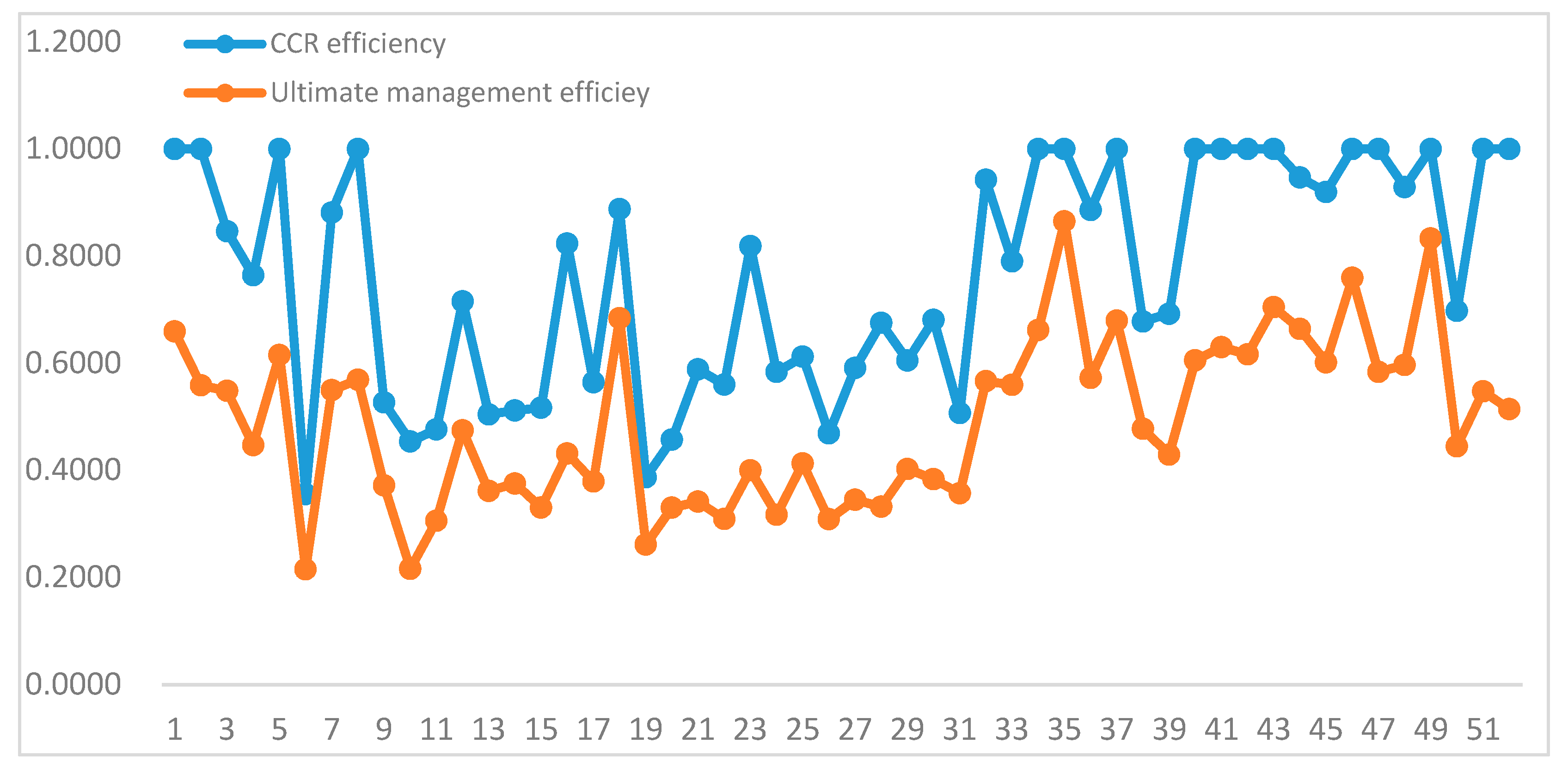
In this case, this study creatively proposes the ultimate comprehensive cross-efficiency evaluation approach (UCCE) with better discriminating ability, which is integrated with two statistical concepts, the Mahalanobis distance and the variation coefficient, such that the numerical characteristics for each criterion can be taken into account and the reliable evaluation results can be produced. We firstly applied it to address the problem of family farm performance evaluation in this work. The management performance evaluation is used to evaluate family farms’ operational efficiency, and their evaluation system consists of utilized agricultural area, labor wages, land rent, machinery operation cost, fertilizer input, pesticide input, and seed input as input measures and crop output value as an output measure. Environmental performance refers to the measurement of relative environmental impact using a measurement system composed of pesticide use per hectare and fertilizer use per hectare as inputs and straw recycling rate as an output index. Family farms are agricultural production units administered by the government, which are at the early stages of development. Each year, the government aims to summarize success and failure and then reward those outstanding family farms to set an example for other farms for improving productivity and reducing negative environmental impacts. In this study, we evaluated family farms’ relative performance and offered a full rank in our proposed UCCE framework. The 35th family farm ranks the first place regarding both management and environmental performance, with performance scores of 0.8648 and 1.0000 while the sixth farm comes bottom concerning management performance with 0.2152 and the 31st farm produces the lowest environmental score of 0.0005. There is weakly positive relationship between the efficiency of the two aspects.

Additionally, we aimed to determine each selected variable’s degree of influence on family farms’ performance. To handle it, we proposed the gray relational analysis. The dependent variable is the estimated score of family farms’ UCCE efficiency (both in terms of management and environmental) and the explanatory variables are their relevant inputs and outputs. For example, we use fertilizer input per hectare, pesticide use per hectare, and straw recycling rate as explanatory variables, while the environmental efficiency score is used as a dependent variable. The result shows that the three explanatory variables have the nearly same degree of influence on environmental performance.

In general, major scientific contribution of this work can be summarized as follows: (i) we firstly designed the evaluation system about family farm’s management and environmental performance and collected the related data of 52 family farms in 2017 in China; (ii) we creatively proposed the UCCE approach to adapt to the issue of family farm’s performance evaluation in this paper; (iii) the relationship between management and environmental performance is investigated and then factors influencing the performance score are further explored and ranked, using gray relational analysis.

The structure of this article includes: The following section summarizes some related literature. The third part depicts the posed means and collected data. The means applies to the fourth section, and then analysis and discussion are conducted. The last part draws some conclusions and discusses the completion of this work.

2. Literature Review

2.1. Studies of Family Farms

Studies on the development of family farm have been conducted by many researchers. In China, family farm is an important modern agricultural microeconomic organization that can liberate productive forces and promote modern agriculture [4]. Han proposed three viewpoints on why family farm is a reasonable agricultural organization for China [29]. First, the natural biological characteristics of agricultural production determine that family management is the most suitable organizational form for agricultural production. Second, family management in agriculture is not equal to small-scale operations, and the scale has gone far beyond the traditional small farm mode. Third, the promotion of the large-scale operation of family farms is needed to achieve agricultural modernization because the long-term protection and consolidation of traditional small-scale agriculture will bar farmers from alleviation of poverty and overall economic development. Zhang thinks that there is room for improvement in the comprehensive development level of China’s planting family farms at present [30]. Family farms have obvious advantages over ordinary farms in terms of labor productivity, land productivity, and pesticide and fertilizer application reduction rates. However, family farms face many risks, such as excessive scale, lack of employed labor, rising production costs, single operating structure, backward social services, and low bargaining power [7].

There are studies focusing on factors that influence the development of family farm. From the point of agricultural inputs, Abay suggested that effective input use often results in sustainability of agriculture and has a positive impact on agricultural production [31]. Zhang proposed that increasing the capital can significantly raise grain yield [32]. Renting more land and implementing a large-scale operation is better for households to obtain a higher technical efficiency [32,33]. Increases in machinery input and effective labor input will reduce distortions, resulting in positive impacts on agricultural production [32,34], and meanwhile human capital plays a major impact on productivity growth [35]. Considering technical environment, the degree of production equipment perfection affects the development of family farm. Regarding social environment, Zhu et al. concluded that government support is necessary for the development of family farm but agricultural subsidies is not an effective measure promoting farmers to be family farmers [36]. Social service environment affects the operation of family farm directly [37].

There are also other factors that contribute to better operation of family farm—educational level of farmers [37,38], management rules and regulations [38], and previous performance [39]. Researchers also pointed out that cultural mode and farmer’s age may have an impact on family farm [40].

Apart from the subject of family farm’s development as an agricultural production unit, some environmental issues are receiving more concern. For example, although chemical inputs such as nitrogen fertilizer and pesticides will significantly increase the yield of crops [41], the indiscriminate use of them have caused serious agriculturally-diffused pollution, which not only damages the ecological environment but also restricts sustainable agricultural development [11]. Another example is that heavy fertilization of greenhouse vegetable bases in China resulted in an accumulation of N, P, Cd, Cu, Pb, and Zn in soil, nutrient eutrophication in irrigation water, and high Cd in some leaf vegetables cultivated in acidic soil [42]. Therefore, to lessen the negative environmental impact of chemical fertilizers, replacing chemical fertilizers with more organic fertilizers is a good choice for farmers. The problem of straw recycling and utilization is also critical. more than 30% of crop straw was burned in the field after harvest in most eastern and southern areas in China [8], emitting large amounts of gaseous and particulate pollutants and leading to greater environmental and social impacts [9,10,43]. Therefore, it is an urgent issue in China to find an environmentally friendly, highly efficient, low cost, and lower secondary pollution-producing approach for straw utilization [43]. It is easier for family farms which operate in a large-scale to find effective solutions addressing the straw utilization issue.

2.2. Research Gap

By summarizing and analyzing the existing research, we found very few studies about management performance evaluation, using China’s family farms as a production unit, have been carried out. Additionally, there is little concern about family farm’s environmental performance, which refers to the negative impact brought by the agricultural production.

As it is a commonly recognized phenomenon that farmers pay too much attention to the improving productivity while almost neglecting the side effects of the production process, it is essential to analyze family farms management together with their environmental performance and provide decision-making information to decision makers such as the government to adopt specific measures to reduce the negative environmental impact.

The operation of a family farm presents unique features due to the influence of natural and human factors, so the diversity of the operation should be considered while during the evaluation process. Given this, we first proposed a novel DEA cross-efficiency approach integrated with two statistical quantities to address the evaluation problem.

In addition, it is necessary to rank selected variables’ degree of influence on family farm performance. Therefore, we applied gray relational analysis (GRA) to investigate and rank the variables impact.

Finally, we investigated further into the connection between family farms’ management and environmental performance and some factors such as the operation scale, crop types, farm owner’s experience, etc.

3. Methods and Data

3.1. Cross Efficiency Evaluation

Suppose there are n DMUs and each DMU_j(j = 1, 2 ..., n) has m different inputs x_ij(i = 1, 2 ..., m) and s different outputs, y_rj(r = 1, 2 ..., s).DEA cross-efficiency is generated by the following two steps:

Step 1: The self-evaluation mode of DEA is represented by the constant return-to-scale (CRS) DEA model by Charnes et al. (1978). The model for DMU_d(d = 1, 2, …, n)’s efficiency evaluation is expressed as

$$\begin{array}{l}\max E_{dd}={\displaystyle \sum _{r=1}^s{u}_{rd}}{y}_{rd}\\ s.t.{\displaystyle \sum _{i=1}^m{v}_{id}}{x}_{ij}-{\displaystyle \sum _{r=1}^s{u}_{rd}}{y}_{rj}\ge 0,j=1,2,\dots ,n.\\ {\displaystyle \sum _{r=1}^m{v}_{id}}{x}_{id}=1.\\ u_{rd}\ge 0,r=1,2,\dots ,s\\ v_{id}\ge 0,i=1,2,\dots ,m,\end{array}$$

(1)

where u_rd and v_id represent the weights for the rth output and ith input for DMU_d, respectively. For each DMU_d, we obtain a set of optimal weights ($v_{1d}^{*},v_{2d}^{*},\dots ,v_{md}^{*},u_{1d}^{*},u_{2d}^{*},\dots ,u_{sd}^{*}$) by solving model (1).

Step 2: Apply the weights derived from Step 1 to all DMUs to obtain the cross-efficiency values of each of the DMUs. We define E_dj as the cross-efficiency of each DMU_j using the optimal weights of DMU_d. The algorithm for calculating E_dj is

$$E_{dj}=\frac{{\displaystyle \sum _{r=1}^s{u}_{rd}^{*}{y}_{rj}}}{{\displaystyle \sum _{i=1}^m{v}_{id}^{*}{x}_{ij}}},d,j=1,2,\dots ,n.$$

(2)

Next, we list the cross-efficiency matrix (CEM) in

Table 1. Cross-efficiency matrix.

Rating DMU	Rated DMU
	1	2	...	n
1	E11	E12	...	E1n
2	E21	E22	...	E2n
...	...	...	...	...
N	En1	En2	...	Enn
Mean	${\stackrel{-}{E}}_1$	${\stackrel{-}{E}}_2$	...	${\stackrel{-}{E}}_n$

.

Then, the traditional cross efficiency value of each DMU_j, $j=1,2,\dots ,n$, an average of all $E_{dj}$ is calculated by

$${\stackrel{-}{E}}_j=\frac{1}{n}{\displaystyle \sum _{d=1}^n{E}_{dj}}$$

(3)

It is obvious that the cross-efficiency value generated by Formula (3) is an average one, which means it treats every evaluation criterion as equal. However, there are at least three shortcomings when the average cross-efficiency is used to evaluate and rank the DMUs:

(1) Averaging cross-efficiency causes a loss of association with the weights [21]. The average cross-efficiency is not the only way to rate the units. One might also consider the range, variance, or the median as alternative ranking factors [24].

(2) The original efficiency score obtained from self-evaluation mode plays a distinctive role in the final overall assessment and ranking, since it lies on the leading diagonal of the CEM [25]. Therefore, it is unreasonable to regard them equally with other cross-efficiency scores.

Due to the simple aggregation method that ignores the relative importance of the cross-efficiency scores, it is often difficult for the average cross-efficiency approach to reveal all the DMUs’ real performance [27].

3.2. Determination of Ultimate Comprehensive Cross-Efficiency

Assume there are k alternatives with t evaluation criteria to be evaluated for decision-making. It is an ideal case for decision makers that each DMU scores with great dissimilarity for each given attribute, because this makes it easy to distinguish and rank all the alternatives. However, the actual conditions do not always cooperate with the ideal case, but are rather complicated.

Zeleny states that, “If all available alternatives scores are approximately equal with respect to a given attribute, then such an attribute will be judged unimportant by most decision makers. Such an attribute does not help in making a decision” [44]. Zeleny’s viewpoint can be applied to evaluate the decision-making units. The decision-making matrix can be expressed as

$$\left(\begin{array}{cccccc}{x}_{11}& x_{12}& \cdots & x_{1i}& \cdots & x_{1t}\\ x_{21}& x_{22}& \cdots & x_{2i}& \cdots & x_{2t}\\ ⋮& ⋮& & ⋮& & ⋮\\ x_{j1}& x_{j2}& \cdots & x_{ji}& \cdots & x_{jt}\\ ⋮& ⋮& & ⋮& & ⋮\\ x_{k1}& x_{k2}& \cdots & x_{ki}& \cdots & x_{kt}\end{array}\right)$$

According to Zeleny, it is reasonable to assign a small weight to the i^th criterion if this criterion generates similar values across all alternatives [24].

In the case of cross-efficiency aggregation, the relationship between our decision-making matrix and the cross-efficiency matrix is:

$$\left(\begin{array}{ccccc}{x}_{11}& x_{12}& x_{13}& \dots & x_{1t}\\ x_{21}& x_{22}& x_{23}& \dots & x_{2t}\\ x_{31}& x_{32}& x_{33}& \dots & x_{3t}\\ \dots & \dots & \dots & \dots & \dots \\ x_{k1}& x_{k2}& x_{k3}& \dots & x_{kt}\end{array}\right)={\left(\begin{array}{ccccc}{E}_{11}& E_{12}& E_{13}& \dots & E_{1n}\\ E_{21}& E_{22}& E_{23}& \dots & E_{2n}\\ E_{31}& E_{32}& E_{33}& \dots & E_{3n}\\ \dots & \dots & \dots & \dots & \dots \\ E_{n1}& E_{n2}& E_{n3}& \dots & E_{nn}\end{array}\right)}^T$$

To evaluate DMU_j under Criterion d(d = 1, 2 ..., n) means to apply the optimal weights of DMU_d to DMU_j and obtain cross-efficiency value E_dj. The dissimilarity of the efficiency values under the rating DMU_d is measured by the variation coefficient, which shows the extent of variability in relation to the mean of efficiency values. Meanwhile, the cross-efficiency evaluation method is used to improve the power of DEA in discriminating the efficient DMUs by incorporating peer evaluation [45]. Therefore, the difference between self-evaluated efficiency and peer-evaluated efficiency should be taken into account. Considering this, the statistical concept of ‘Mahalanobis distance’ is employed to measure the difference between this study and the viewpoint that the impact of each column’s unit in Table 1 should be reduced.

3.2.1. Principle of the UCCE Approach

Considering the research subject in this study, the principle of this proposed method is assigning aggregation weights corresponding to the digital features, including the variation coefficient and the Mahalanobis distance of each criterion. The operation of family farms presents unique features due to the influence of natural and social factors, which means that each family farm has a group of particular input-output data. Each time we evaluate a family farm’s performance by model (1), we would obtain a corresponding set of optimal weights. In the cross-efficiency evaluation approach, we take each set of optimal weights as an evaluation criterion for all DMUs (family farms). For the purpose of the objectivity of a family farm’s performance evaluation, it is reasonable to apply weights in accordance with the digital features of the criterion described above.

3.2.2. Calculation Procedure of UCCE

Finally, the procedure for the calculation of the proposed UCCE approach is defined as

Step 1. We define $P_d(x_1,x_2,\dots ,x_3)=(E_{d1},E_{d2},\dots ,E_{dj},\dots ,E_{dn})$ for rating DMU_d and $O=\left(E_{11},E_{22},\dots E_{jj},\dots ,E_{nn}\right)$ for the self-evaluation CCR score. Both P_d and O are points in the N-dimensional Euclidean space.

Step 2. Calculate the difference between self-evaluated efficiency and peer-evaluated efficiency using the Mahalanobis distance between point P_d and O

$$\begin{array}{l}d(O,P_d)=d_{P_d}=\sqrt{\frac{{(E_{d1}-E_{11})}^2}{{\sigma }_1}+\frac{{(E_{d2}-E_{22})}^2}{{\sigma }_2}+\dots +\frac{{(E_{dj}-E_{jj})}^2}{{\sigma }_j}+\dots +\frac{{(E_{dn}-E_{nn})}^2}{{\sigma }_n}}\\ d=1,2,\dots ,n\end{array}$$

(4)

where ${\sigma }_j$ represents the variance of the rated DMU_j’s cross-efficiency scores,

$${\sigma }_{\mathrm{j}}=\frac{1}{n}{\displaystyle \sum _{d=1}^n{(E_{dj}-{\stackrel{-}{E}}_j)}^2},j=1,2,\dots ,n$$

$${\sigma }_{\mathrm{j}}=\frac{1}{n}{\displaystyle \sum _{d=1}^n{(E_{dj}-{\stackrel{-}{E}}_j)}^2},j=1,2,\dots ,n,$$

and

$${\stackrel{-}{E}}_j=\frac{1}{n}{\displaystyle \sum _{d=1}^n{E}_{dj}},j=1,2,\dots ,n.$$

Step 3. The variation coefficient for rating DMU_d is expressed by

$${\delta }_d=\frac{{\sigma }_d}{{\stackrel{-}{E}}_d},d=1,2,\dots ,n.$$

(5)

where the standard deviation value for rating DMU_d is calculated by

$${\sigma }_{\mathrm{d}}=\sqrt{\frac{1}{n}{\displaystyle \sum _{j=1}^n{(E_{dj}-{\stackrel{-}{E}}_d)}^2}},d=1,2,\dots ,n,$$

and

$${\stackrel{-}{E}}_d=\frac{1}{n}{\displaystyle \sum _{j=1}^n{E}_{dj}},d=1,2,\dots ,n.$$

Step 4. Normalize the sequence of the Mahalanobis distance and the sequence of coefficient variation to avoid the impacts of units.

$$\begin{array}{l}{d}_{{\mathrm{p}}_d}^{nrm}=\frac{d_{{\mathrm{p}}_d}-d_{{\mathrm{p}}_d}^{\min }}{d_{{\mathrm{p}}_d}^{\max }-d_{{\mathrm{p}}_d}^{\min }},\\ {\delta }_d^{nrm}=\frac{{\delta }_d-{\delta }_d^{\min }}{{\delta }_d^{\max }-{\delta }_d^{\min }},\\ d=1,2,\dots ,n\end{array}$$

Step 5. The weights to aggregate the cross-efficiency scores of DMU_j(j = 1, 2 ..., n) are defined as

$${\lambda }_d=\frac{{\delta }_d^{nrm}{d}_d^{nrm}}{{\displaystyle \sum _{d=1}^n{\delta }_d^{nrm}{d}_d^{nrm}}},d=1,2,\dots ,n.$$

(6)

The weights derived from Formula (6) take both the distance and the variation coefficient of a criterion into account. The larger the value of parameter λ_d is, the more important the criterion is.

Consequently, the ultimate comprehensive cross-efficiency can be aggregated as

$$E_j^{cross}={\displaystyle \sum _{d=1}^n{E}_{dj}}{\lambda }_d,j=1,2,\dots ,n.$$

(7)

3.3. Gray Relational Analysis

Gray relational analysis is one of the most widely used models of gray system theory that has been applied in various fields of engineering and management [46,47,48]. The agricultural production system is actually a gray system with incomplete information. Family farms are a representative agricultural production unit. Therefore, we apply GRA to investigate the production variables’ impacts on family farms’ performance in this study.

When the units in which a DMU is measured are different for different variables, the influence of some variables may be neglected. This may be the case if some performance variables have a very large range [49]. Therefore, it is necessary to process all performance values of every DMU into a comparability sequence by a process analogous to equalization. For an efficiency-determination problem, both inputs and outputs are potential variables that influence the ultimate efficiency, and we regard each DMU as an observation. The GRA is used to rank important variables that affect the efficiency of DMUs. If there are m variables and n observations, the ith variable can be expressed as X_i(i = 1, 2 ..., m). The observed data of the cross-efficiency and variables are shown as

$$\left(\begin{array}{cccccc}{x}_{11}& x_{12}& \cdots & x_{1j}& \cdots & x_{1n}\\ x_{21}& x_{22}& \cdots & x_{2j}& \cdots & x_{2n}\\ ⋮& ⋮& & ⋮& & ⋮\\ x_{i1}& x_{i2}& \cdots & x_{ij}& \cdots & x_{in}\\ ⋮& ⋮& & ⋮& & ⋮\\ x_{m1}& x_{m2}& \cdots & x_{mj}& \cdots & x_{mn}\\ E_1^{cross}& E_2^{cross}& \cdots & E_j^{cross}& \cdots & E_n^{cross}\end{array}\right)$$

where $x_{ij}\left(j=1,2,\dots ,n\right)$ is the observed value of the i^th variable and $E_j^{cross}$ is the cross-efficiency value. The term X_i can be translated into a comparable sequence $X_i=\left\{x_i^{(0)}(1),x_i^{(0)}(2),\cdots ,x_i^{(0)}(j),\cdots ,x_i^{(0)}(n)\right\},i=1,2,\cdots ,m$ by $x_i^{(0)}(j)=\frac{x_{ij}}{\underset{j=1,\dots ,n}{\max }\left\{x_{ij}\right\}},j=1,2,\cdots ,n$ in order to reduce the impact of different units, where $\stackrel{-}{x_i}$ is the mean value of the n observations of X_i. Meanwhile, the efficiency sequence is transformed in the same way:

$$E_{}^{(0)}(j)=\frac{E_j^{cross}}{\max \left\{E_j^{cross}\right\}},j=1,2,\cdots ,n.$$

Let $M=\{1,2,\cdots ,m\}$, $N=\{1,2,\cdots ,n\}$.

We denote:

$${\Delta }_1=\underset{i\in M}{\min }\left\{\underset{j\in N}{\min }\left|E_{}^{(0)}(j)-x_i^{(0)}(j)\right|\right\},$$

$${\Delta }_2=\underset{i\in M}{\max }\left\{\underset{j\in N}{\max }\left|E_{}^{(0)}(j)-x_i^{(0)}(j)\right|\right\},$$

$${\Delta }_3=\left|E_{}^{(0)}(j)-x_i^{(0)}(j)\right|,$$

$$d_{0i}(j)=\frac{{\Delta }_1+\alpha {\Delta }_2}{{\Delta }_3+\alpha {\Delta }_2},j=1,2,\cdots ,n.$$

where $d_{0i}(j)$ is the GRA coefficient between $E_{}^{(0)}(j)$ and $x_i^{(0)}(j)$, and α is the distinguishing coefficient, $\alpha \in [0,1]$.

Deng stated that the value of 0.5 is normally applied [50]. After calculating for the gray relational coefficient $d_{0i}(j)$, the gray relational grade can then be calculated as

$$r_{0i}={\displaystyle \sum _{j=1}^n{w}_j{d}_{0i}(j)},i\in M.$$

(8)

Here, $w_j$ denotes the normalized weight of criterion j, where ${\displaystyle \sum _{j=1}^n{w}_j}=1$ with equal weights. The proposed methodology, which applies GRA to rank the most important variable with respect to family farms’ performance, is thus developed. The rank-ordering algorithm is applied to determine the ranking of the variables.

The gray relational grade indicates the degree of similarity between the comparability sequence and the reference sequence [50]. In this case, if a comparability sequence for a certain variable obtains the highest gray relational grade with the UCCE efficiency sequence, this means that the variables have the largest influence on family farms’ performance, and these variables are the most important. 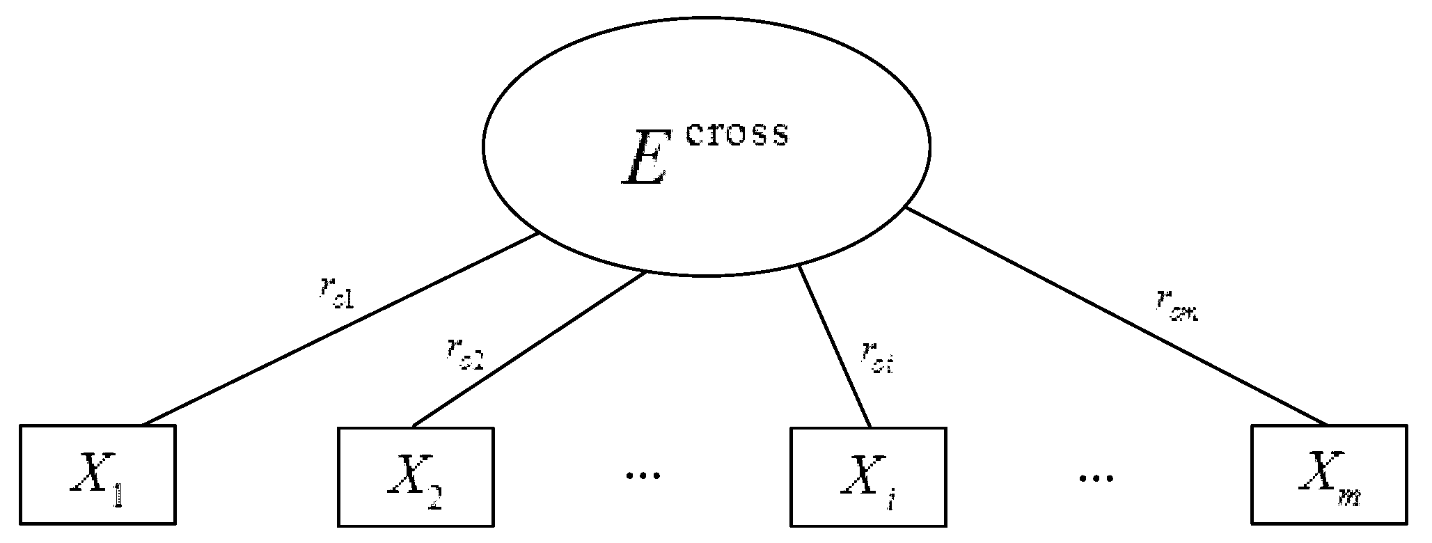Figure 1 shows the relationship between cross-efficiency and relevant variables.

3.4. Data Collection

We chose a sample of 52 representative family farms that distribute across Jilin and Shandong provinces and produce various grain crops, including corn, rice, wheat, sorghum, soybean, etc.

Field investigation and face-to-face interviews were carried out with farm owners, members and local agricultural enterprises. The data used in this paper are obtained from operations in 2017, and each family farm is considered as an independent DMU.

Two regional differences affecting agricultural production between the two provinces are summarized as follows: (i) one season crop in Jilin, two seasons in Shandong due to the temperature difference; and (ii) family farms in Jilin has larger land area, and conduct more intensive and large-scale operation than Shandong.

3.4.1. Variables for Management Performance Evaluation

For illustrative purpose and without a loss of generality, seven inputs and one desirable output, which cover the whole production activity of family farms, are selected to evaluate family farms’ management performance.

Table 2. Variables for management performance evaluation

No.	Type	Name	Units
1	Input	Utilized Agricultural Area (UAA)	Hectare
2		Labor Wages (LW)	104 CNY
3		Land Rent (LR)
4		Machinery Operation Cost (MOC)
5		Fertilizer Input (FI)
6		Pesticide Input (PI)
7		Seed Input (SI)
8	Output	Crop Output Value (COV)

shows all the variables selected. Labor Wages were quantified as the total value of RMB spent for family farms’ labor use (family workers and independent workers, both permanent and temporary) in each operation related to agricultural production. Utilized agricultural area is the operation area of a family farm. It is the total area that every family farm produces crops on. Land rent is the RMB cost of the UAA. A family farm’s own land is regarded as equal to their contracted land, both of which are priced according to the market conditions at that time. Machinery operation cost is determined by the expense (RMB) of renting large agricultural machines and the cost of irrigation. Fertilizer input includes expenditures on all kinds of fertilizers (RMB), which have different impacts and contributions during the crop growth stage. Pesticide input refers to the expenditures (RMB) of all pesticides used throughout the whole crop growth stage. Seed input is the cost (RMB) of crop seeds (such as corn seeds) or seedlings (such as rice seedlings) at the preliminary stage. The crop output value is the only desirable output selected. We use the crop yield multiplied by the market price to get this indicator, which reflects family farms’ yearly outcomes.

3.4.2. Variables for Environmental Performance Evaluation

We selected two inputs and one output, as are shown in

Table 3. Variables for environmental performance evaluation

No.	Type	Name	Units
1	Input	Fertilizer Input Per Hectare (FIPH)	CNY
2		Pesticide Input Per Hectare (PIPH)
3	Output	Straw Recycling Rate (SRR)	Ratio

, to evaluate the 52 family farms’ environmental performance: the fertilizer input per hectare (FIPH) and pesticide input per hectare (PIPH) as input indicators, and the straw recycling rate (SRR) as the output indicator. The three selected variables cover the environmental issues in the field of agriculture that receive the greatest attention from both the government and the public in China.

As a variety of fertilizers and pesticides that function differently are applied during the crop growth stage, it is not wise to simply add them together by their weight. Therefore, we calculate the fertilizer input and pesticide input per hectare by Chinese Yuan (CNY) based on the analysis of field research that more spent on fertilizers and pesticides means less concern about the negative impact on the environment for each family farm.

The SRR is the occupation proportion of appropriately disposed of straw of the total amount produced. This variable is defined as a ratio with a value between 0 and 1, theoretically, and it can be equal to 0 or 1. The observed data of the SRR is between 0 and 1.0. Straw that is appropriately disposed of is straw that is sent to power plants, crushed to be used as fertilizer for the farmland or reused as cattle feed instead of being burned directly without any decontamination measures.

4. Results and Discussion

4.1. Descriptive Statistics

Table 4. Descriptive statistics of the input and output variables of the sample (n = 52)

Inputs/Outputs	Variable	Min	Max	Mean	Standard Deviation	Variation Coefficient
Input	LW	1	28.53	8.87	7.38	0.83
	UAA	2	220	55.13	51.14	0.93
	LR	1	180	31.76	37.63	1.18
	MOC	0.26	39.36	9.38	9.01	0.96
	FI	0.24	36.85	10.26	9.97	0.97
	PI	0.1	12.65	2.84	2.82	0.99
	SI	0.28	34	5.3	7.62	1.44
	FIPH	600	4300	1880.19	781.06	0.42
	PIPH	97.94	2400	615.17	400.01	0.65
Output	SRR	0	1	0.75	0.26	0.34
	COV	3.24	560	103.16	110.89	1.07

shows the descriptive statistics of our collected input-output data. Regarding outputs, the 52 grain family farms had an average crop output value of 103.16 × 10⁴ yuan and an average straw recycling rate of 0.75. Both outputs presented high variability among the farms considered, as they showed the magnitude of the min-max range and the variation coefficient values. Regarding inputs, the average utilized agricultural area of the farms is 55.13 hectares, with a minimum of 2 hectares for the smallest farm, up to a maximum of 220 hectares for the most extensive farm. Regarding labor wages, on average, the sampled farms devoted approximately 8.87 × 10⁴ yuan for agricultural production activities, with differences between farms related to utilized agricultural area and crop species. Regarding land rent, sampled farms spent approximately 31.76 × 10⁴ yuan on average with differences related to utilized agricultural area and the local land circulation market. As for fertilizer input and pesticide input, the average quantities were 10.26 × 10⁴ and 2.84 × 10⁴ yuan, respectively, and varied between 0.24 × 10⁴ to 36.85 × 10⁴ yuan for FI and 0.10 × 10⁴ to 12.65 × 10⁴ yuan for PI depending on the crop species, land condition, and the applied technology, such as variable fertilization techniques. The fertilizer input per hectare and pesticide input per hectare varied from 600 yuan to 4300 yuan and 97.94 yuan to 2400 yuan, respectively, with the average values of 1880.19 and 615.17 yuan, respectively. The machinery operation cost had an average value of 9.38 × 10⁴ yuan with a minimum of 0.26 × 10⁴ yuan to a maximum of 39.36 × 10⁴ yuan, with high variability within the sample.

4.2. Results and Discussion

4.2.1. Preliminary Results

The CCR efficiency is acquired from model (1) and the average cross-efficiency results are derived from Formula (3). The preliminary results are given in

Table 5. CCR efficiency and average cross-efficiency results

Family Farms	CCR Efficiency Evaluation Results				Average Cross-Efficiency Evaluation Results
	Management Performance	Rank	Environmental Performance	Rank	Management Performance	Rank	Environmental Performance	Rank
1	1	1	0.5672	23	0.6811	12	0.5335	20
2	1	1	0.6667	17	0.5632	25	0.6168	15
4	0.764	10	0.7333	10	0.4546	32	0.7053	7
5	1	1	0.2188	47	0.6447	15	0.2082	47
6	0.3556	26	0.7333	10	0.2372	52	0.7053	7
7	0.881	6	0.5175	30	0.5654	24	0.4811	27
8	1	1	0.1592	50	0.5841	21	0.1483	50
33	0.7901	27	0.4393	32	0.6137	19	0.4232	29
34	1	1	0.7308	14	0.7195	6	0.7128	5
35	1	1	1	1	0.9273	1	1	1
37	1	1	1	1	0.7185	7	0.5805	18
39	0.6923	31	0.55	26	0.4649	29	0.5111	22
40	1	1	0.3901	35	0.688	10	0.3702	35
41	1	1	0.309	40	0.7154	8	0.3002	40
42	1	1	0.2921	42	0.7026	9	0.2837	41
43	1	1	0.9114	5	0.7526	5	0.867	3
44	0.9467	17	0.4231	33	0.683	11	0.4004	33
46	1	1	0.5823	22	0.7854	3	0.5501	19
47	1	1	0.7097	16	0.6582	14	0.4195	30
48	0.9287	19	0.3667	36	0.6757	13	0.3431	36
49	1	1	0.6535	19	0.9216	2	0.6122	16
51	1	1	0.8879	6	0.618	18	0.6485	14
52	1	1	0.6099	20	0.5821	22	0.4066	31

Note: the results of all 52 family farms are shown in the Appendix A.

.

In regard to CCR efficiency, it is notable from Table 5 that some family farms (1, 2, 5, 8, 34, 35, 37, 40, 41, 42, 43, 46, 47, 49, 51, and 52) have the same management efficiency score of 1.0000 and the same ranking order of 1. With this self-evaluation approach, it is difficult to distinguish which family farm performs better than the others. Regarding environmental performance, there are only two family farms (35 and 36) that reach the efficient performance value of 1.0000, which shows quite a different appearance because of the comparably fewer input-output variables than the management performance evaluation.

4.2.2. Ultimate Comprehensive Cross-Efficiency

We define the evaluation results of our proposed approach as ultimate comprehensive cross-efficiency (or ultimate cross-efficiency). By conducting the working procedure of our proposed approach, we obtain some related process data and some of the results displayed in

Table 6. Determination of UCCE weight (10 out of 52 criteria (Rating DMUs)).

	Criterion	Variation Coefficient	Mahalanobis Distance	Normalized_ Variation Coefficient	Normalized_ Mahalanobis Distance	Ultimate Weight
Management performance	1	0.583	6.7273	0.5593	0.6035	0.0328
	2	0.6269	7.1783	0.6014	0.644	0.0377
	3	0.4265	4.9733	0.4091	0.4462	0.0178
	4	0.6071	7.0366	0.5825	0.6313	0.0358
	47	0.4074	4.1064	0.3909	0.3684	0.0140
	48	0.3561	4.2316	0.3416	0.3796	0.0126
	49	0.3465	3.7292	0.3325	0.3346	0.0108
	50	0.4433	5.6140	0.4253	0.5036	0.0208
	51	0.4052	4.0369	0.3887	0.3622	0.0137
	52	0.4221	4.4375	0.4050	0.3981	0.0157
Environmental performance	1	0.4610	2.2418	0.7145	0.4685	0.0206
	2	0.4610	2.2418	0.7145	0.4685	0.0206
	3	0.4610	2.2418	0.7145	0.4685	0.0206
	4	0.4610	2.2418	0.7145	0.4685	0.0206
	47	0.6452	4.7855	1.0000	1.0000	0.0440
	48	0.4610	2.2418	0.7145	0.4685	0.0147
	49	0.4610	2.2418	0.7145	0.4685	0.0147
	50	0.4610	2.2418	0.7145	0.4685	0.0147
	51	0.6452	4.7855	1.0000	1.0000	0.0440
	52	0.6452	4.7855	1.0000	1.0000	0.0440

.

The variation coefficient and Mahalanobis distance are calculated by Equations (5) and (4), respectively. The last column of Table 6 displays the UCCE weight, which is determined by Equation (6). The higher the ultimate weight, the greater the importance of the cross efficiency of criterion j (Rating DMU_j). Take Rating DMU₅ and DMU₇ for instance: regarding management performance, rating DMU₇ has a Mahalanobis distance value of 7.3122, almost twice that of Rating DMU₅, which is 3.9266. Meanwhile, the variation coefficient of Rating DMU₇ is 0.6379, which is also larger than the 0.3789 of DMU₅. Therefore, after the normalization process calculated by Equation (6), Rating DMU₇ has a relatively higher ultimate weight (0.0391) than Rating DMU₅ (0.0125). The above example shows that the ultimate weights derived from our approach are in accordance with Zeleny’s viewpoint about decision-making and Sexton’s idea concerning the reduction of self-evaluation modes.

It is easy to recognize that our approach provides more reliable ultimate cross-efficiency weights that consider both the statistical distance and the variation coefficient. The ultimate efficiency evaluation results are shown in

Table 7. UCCE results.

Family Farms	UCCE Results				Family Farms	UCCE Results
	Management Performance	Rank	Environmental Performance	Rank		Management Performance	Rank	Environmental Performance	Rank
1	0.6591	9	0.4901	23	27	0.3449	41	0.2932	38
2	0.5588	21	0.5527	17	28	0.3323	43	0.2388	43
3	0.5484	23	0.452	29	29	0.4025	33	0.3623	33
4	0.4469	28	0.6692	9	30	0.3833	35	0.1537	49
5	0.6151	12	0.1945	47	31	0.3573	40	0.0005	52
6	0.2152	52	0.6692	9	32	0.5665	19	0.4915	22
7	0.5495	22	0.4342	30	33	0.5597	20	0.4026	31
8	0.5692	18	0.1342	50	34	0.6618	8	0.6896	7
9	0.372	38	0.7381	4	35	0.8648	1	1.0000	1
10	0.2162	51	0.5161	19	36	0.5727	17	0.5163	18
11	0.3059	49	0.6143	14	37	0.6796	6	0.6788	8
12	0.4747	27	0.2486	42	38	0.4775	26	0.7348	5
13	0.3613	39	0.5756	15	39	0.4293	31	0.4611	26
14	0.3754	37	0.2873	40	40	0.6053	13	0.3446	34
15	0.3303	45	0.231	44	41	0.63	10	0.2889	39
16	0.4314	30	0.0799	51	42	0.6164	11	0.2729	41
17	0.3792	36	0.2168	45	43	0.7046	4	0.8099	3
18	0.6839	5	0.6375	12	44	0.6639	7	0.3713	32
19	0.2612	50	0.3086	37	45	0.6016	14	0.6655	11
20	0.3304	44	0.4803	25	46	0.7593	3	0.5086	20
21	0.3416	42	0.1909	48	47	0.5836	16	0.4874	24
22	0.3091	47	0.3295	35	48	0.5969	15	0.3126	36
23	0.4001	34	0.2023	46	49	0.8327	2	0.5591	16
24	0.3172	46	0.4575	27	50	0.445	29	0.6375	12
25	0.4129	32	0.4978	21	51	0.5475	24	0.7046	6
26	0.3087	48	0.8150	2	52	0.5142	25	0.4542	28

.

The management performances for all 52 family farms are rated from 0.2152 to 0.8648, with Farm 6 being the least efficient family farm and Farm 35 being the most efficient family farm. Regarding environmental performance, farm 40 has the lowest efficiency score, 0.0005, and the highest is 1.0000 for Farm 35.

4.3. Methodology Comparison and Discussion

4.3.1. CCR efficiency and UCCE Efficiency

Figure 2 and Figure 3 compare the traditional CCR management efficiency and ultimate management efficiency for all 52 family farms. As seen, the ultimate cross-efficiency scores are lower than the CCR efficiency scores, from both the management and environmental perspective. This reduction is mainly due to the integration of peer-evaluation ideas and the consideration of the unique features of each criterion.

4.3.2. Average Cross-Efficiency and UCCE Efficiency

Figure 4 exhibits the ranking order changes of family farm performance while adopting two different approaches: the traditional average cross-efficiency method and the UCCE approach. There are significant changes in ranking order regarding both management and environmental performance. Twenty-five of 52 family farms’ ranking order changed in both performance evaluations, while a total of 37 and 36 farms changed in terms of management and environmental performance, respectively. The variation range varied between −8 and +10, which demonstrates a significant adjustment since our approach will not change the cross-efficiency ranking arbitrarily but is based on the specific reasons and full consideration of the quantitative information contained in the cross-efficiency matrix. It is also notable that some family farms (19, 21, 30, and 35) maintain their rank order stably, no matter whether the average efficiency is changed into UCCE efficiency.

4.3.3. Comparison of Distinguishing Ability

It is easy to find in Figure 5 that the UCCE method resulting in a higher variation coefficient value than the CCR efficiency and average cross-efficiency approaches. Meanwhile, regarding the discriminative ability of our approach (see Table 5 and Table 7), which has significantly reduced the number of efficient DMUs, our approach obtained reliable and more distinctive results for decision makers.

4.4. Performance Analysis

As is shown in

Table 8. Statistical characteristics of management and environmental efficiency.

	Management Efficiency	Environmental Efficiency
Min	0.2152	0.0005
Max	0.8648	1.0000
Mean	0.4905	0.4512
Variation coefficient	0.3184	0.4706

, the management efficiency of the 52 family farms varied, with a minimum value of 0.2152 to a maximum value of 0.8648, and its average value is 0.4905. Compared to management efficiency, the environmental efficiency ranges in value from 0.0005 to 1.00, which is wider than family farms’ management performance range. Moreover, the environmental efficiency scores have larger variation coefficients than management efficiency.

Additionally, we can learn from Figure 6 that there seems to be weak connection between management and environmental efficiency. To demonstrate our assumption, a Pearson correlation coefficient was calculated, and the results show a score of 0.2914 > 0, indicating a weakly positive correlation, which is in favor of our opinion.

4.4.1. Analysis of Performance and Planted Crops

A variety of crop species are planted by family farms, such as corn, rice, wheat, sorghum, soybeans, etc. Each family farm grows one or a combination of these crops. To investigate the relationship between family farms and the number of crops planted, we divided all 52 selected family farms into two types, including the single type, which refers to those that grow one certain crop, and the mixed type, which refers to those that grow several (≥2) crops.

Table 9. Top 10 family farms regarding management performance.

Top 10 Family Farms	Management Efficiency	Rank	Environmental Efficiency	Rank	Type
35	0.8648	1	1.0000	1	mixed
49	0.8327	2	0.5591	16	mixed
46	0.7593	3	0.5086	20	single
43	0.7046	4	0.8099	3	mixed
18	0.6839	5	0.6375	12	mixed
37	0.6796	6	0.6788	8	single
44	0.6639	7	0.3713	32	mixed
34	0.6618	8	0.6896	7	mixed
1	0.6591	9	0.4901	23	mixed
41	0.6300	10	0.2889	39	mixed

shows the top 10 family farms in terms of their management performance, while

Table 10. Last 10 family farms regarding management performance.

Last 10 Family Farms	Management Efficiency	Rank	Environmental Efficiency	Rank	Type
28	0.3323	43	0.2388	43	mixed
20	0.3304	44	0.4803	25	single
15	0.3303	45	0.2310	44	single
24	0.3172	46	0.4575	27	single
22	0.3091	47	0.3295	35	single
26	0.3087	48	0.8150	2	single
11	0.3059	49	0.6143	14	single
19	0.2612	50	0.3086	37	single
10	0.2162	51	0.5161	19	mixed
6	0.2152	52	0.6692	9	single

shows the bottom 10 farms. It is notable that eight farms are mixed types and there are only two exceptions, Farms 46 and 37. The reason they rank at the front even though they do not adopt the mixed-type strategy is that they cooperate with food companies, such as McDonald’s, which provide higher food prices for them than the market in exchange for a production process that is conducted within the provided standards of the company.

The agricultural product market is not stably operated in China, and the prices of agricultural products usually fluctuate a lot on a yearly basis. It is a risky action to cultivate just one crop in great amounts because it might cause deficits due to the unreasonable price. Considering this, farms (such as farms 35, 49, 43, 18, 44, 34, 1, and 41) usually cultivate several types of crops at the same time to avoid the risks mentioned above. However, it is not the case that more types of crops planted corresponds with more profits. Increasing the types of crops requires the farm owner to have a good knowledge of planting techniques and wealthy experience with farm management. Otherwise, the opposite effects would be caused, such generating a great deal of cost. For example, farmers who used to be sellers of agricultural material and those who have previous experience operating large amounts of land tend to operate family farms smoothly. Those who switched from another industry directly and lack related knowledge and experience always face the embarrassing situation of deficit.

4.4.2. Performance Analysis Regarding Different Scales

Liu divided the operational area of family farms in four sections: 0–6.67 ha., 6.67–66.7 ha., 66.7–200 ha. and >200 ha according to the degree of mechanization [51]. In line with that research, we divided the 52 family farms into four groups (

Table 11. Performance values in different scales.

Utilized Agricultural Area	Number of Family Farm	Management Performance Score	Environmental Performance Score
>200 ha.	1	0.6591	0.4901
66.7–200 ha.	15	0.5909	0.4842
6.67–66.7 ha.	30	0.4671	0.4586
0–6.67 ha.	6	0.3285	0.3254

Note: The performance scores given in Table 12 are averaged values.

), and each group contained family farms 6, 30, 15, and 1. Surprisingly, we found that both the average management and environmental performance value have a trend of increasing in correspondence with the size of the family farm (Table 11). Oduol suggested that increasing the scale of operation is necessary if the households have to improve technical efficiency [52]. Likewise, small farms are found to be less allocatively efficient than medium and large farms. Figure 7 shows the performance score in different scales.

4.4.3. Performance Analysis Regarding Regional Differences

For the purpose of figuring out the difference of family farms’s performance regarding regional difference, one-way analysis of variance with a significant level of 0.01 was conducted. Number of observations of Shandong and Jilin Province is 31 and 21 respectively.

Considering the Management performance, an average score of 0.4063 and 0.6149 is obtained for Shandong and Jilin Province, drawing the conclusion that a more effective operation of family farms is carried out in Jilin rather than Shandong. F = 38.9815 > F crit = 7.1706 further reveals the difference with a significant level of 0.01. Regarding the environmental performance, average performance score of Shandong is 0.3894 whereas 0.5425 of Jilin, which means family farms in Jilin perform better than those in Shandong on average. F = 7.3098 > F crit = 7.7106 shows a notable difference lies in family farms between the two provinces at the significant level of 0.01. All in all, notable differences of family farms between the two provinces are identified and Jilin performs better than Shandong both in management and environmental performance, based on the data of the 52 selected family farms.

4.5. Variable Importance Analysis

4.5.1. Variable Importance for Management Performance

The gray relational grade of each variable in

Table 13. Variables’ ranking order in terms of management performance.

Variables	Gray Relational Grade	Rank
LW	0.6165	1
UAA	0.5869	3
LR	0.5415	7
MOC	0.5803	4
FI	0.6066	2
PI	0.5689	5
SI	0.5176	8
COV	0.5504	6

and

Table 14. Variables’ ranking order corresponding to environmental performance.

Variables	Gray Relational Grade	Rank
FIPH	0.6506	1
PIPH	0.6387	2
SRR	0.6321	3

is calculated by Equation (8), of which the ranking indicates the variables’ relative impact on the UCCE efficiency. One of the possible explanations of this result instead of another different one is that we adopted the outcome of UCCE approach, which evaluate DMU in a more comprehensive and objective way as the dependent variable and the relevant production data as independent variable.

The ranking order of the eight variables provides sufficient information for management performance improvement. Firstly, variable LW ranks as the most important factor, verifying Zhang’s viewpoint that human capital plays a major role in productivity growth [53]. FI ranks the second among all variables. Fang studied buckwheat production and found that nitrogen fertilizer is one of the crucial factors that affects the yield of common buckwheat [41]. In this case, FI also plays a significant role. The third important variable is the UAA whose gray relational grade is 0.5869. Studies have shown that increasing the scale of operation can also increase technical efficiency at the same time [32,33]. It is shown in Table 13 that MOC ranks fourth in relation to ultimate cross-efficiency. Increase in machinery input usually results in higher technical efficiency [34]. PI ranks fifth and COV ranks sixth, followed by the LR and SI, which rank seventh and eighth, respectively. The reason why SI ranks the bottom of the eight variables may be that its input amount is relatively fixed and seed usually have a unified retail price.

4.5.2. Variable Importance for Environmental Performance

The three variables show a ranking of gray relational grades of 0.6506, 0.6387, and 0.6321 for fertilizer input per hectare, pesticide input per hectare and straw recycling rate, respectively. It is almost the same scores for the three selected variables, especially for PIPH and SRR. The outcome reflects that efforts towards environmental performance improvement would receive almost the same effect, focusing on the three aspects, FIPH, PIPH, and SRR.

Cao indicates that the government can increase the cost of pesticides by levying pesticide taxes to encourage farmers to choose ecological planting approaches or increase the price of pesticides to increase the incentives for farmers to adopt ecological planting technology [54]. In our opinion, the government can also introduce new production technology and provide necessary training for farmers to reduce fertilizer and pesticide input. For the disposing and recycling of crop straw, there is a strong requirement for subsidies from the government for family farms because it is very costly with little reward at this stage.

5. Conclusions

Family farms are important production organizations that contribute to realizing China’s agricultural modernization. At present, China’s agriculture has not yet fully achieved large-scale production and is still in the development phase. At this phase, family farms play a vital role as a new agricultural production entity and they will have a large impact on China’s economy.

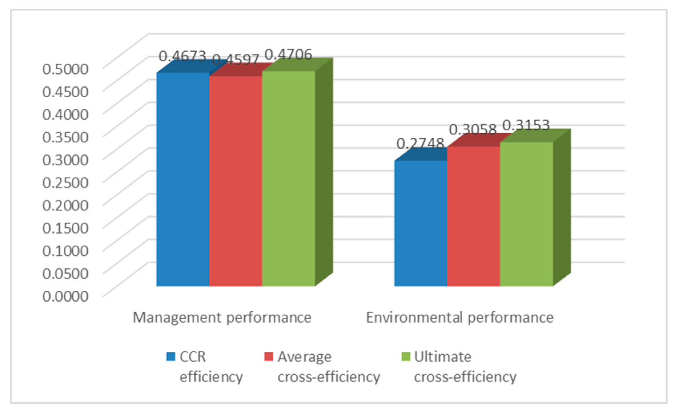
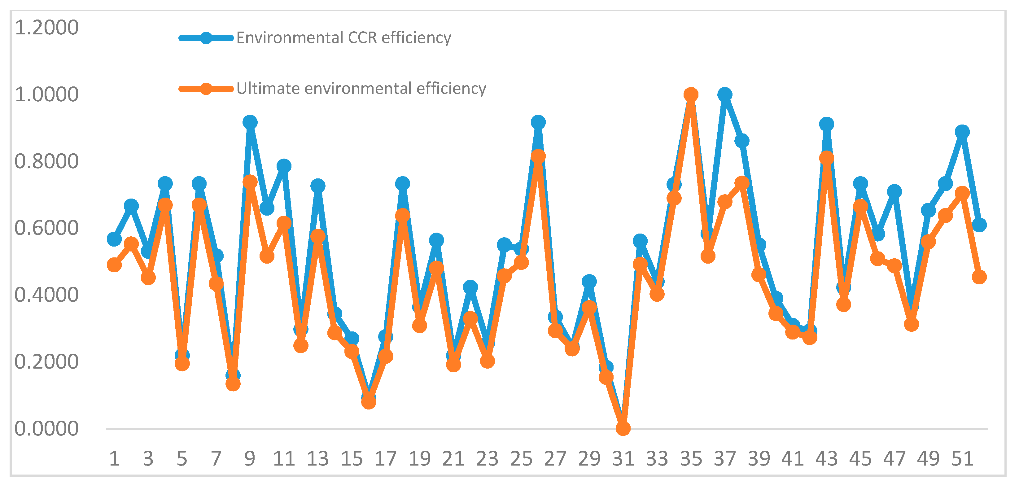
In line with the family farm performance evaluation issue, we modified the DEA cross-efficiency approach (UCCE) by taking unique features of family farms into consideration. Regarding the use of each rating DMU’s optimal weight as an evaluation criterion, we assigned reasonable weights to each criterion and took into account the two statistical quantities, variation coefficient and Mahalanobis distance. The evaluation results show a significant improvement contributed by our proposed approach from multiple perspectives:

(1)

It effectively reduces the number of efficient DMUs.

(2)

The results of our ultimate cross-efficiency generate the highest variation coefficient compared with CCR efficiency and average cross-efficiency.

(3)

It lowers the CCR efficiency value due to the reduction of the impact of self-evaluation.

The main reasons for the above improvements are that our approach takes the diversity of the evaluation results into account, as suggested by Zeleny. Regarding the cross-efficiency matrix, the diversity of the evaluation results is expressed by the variation coefficient of each row and the Mahalanobis distance between CCR efficiency results and each row of the cross efficiency matrix.

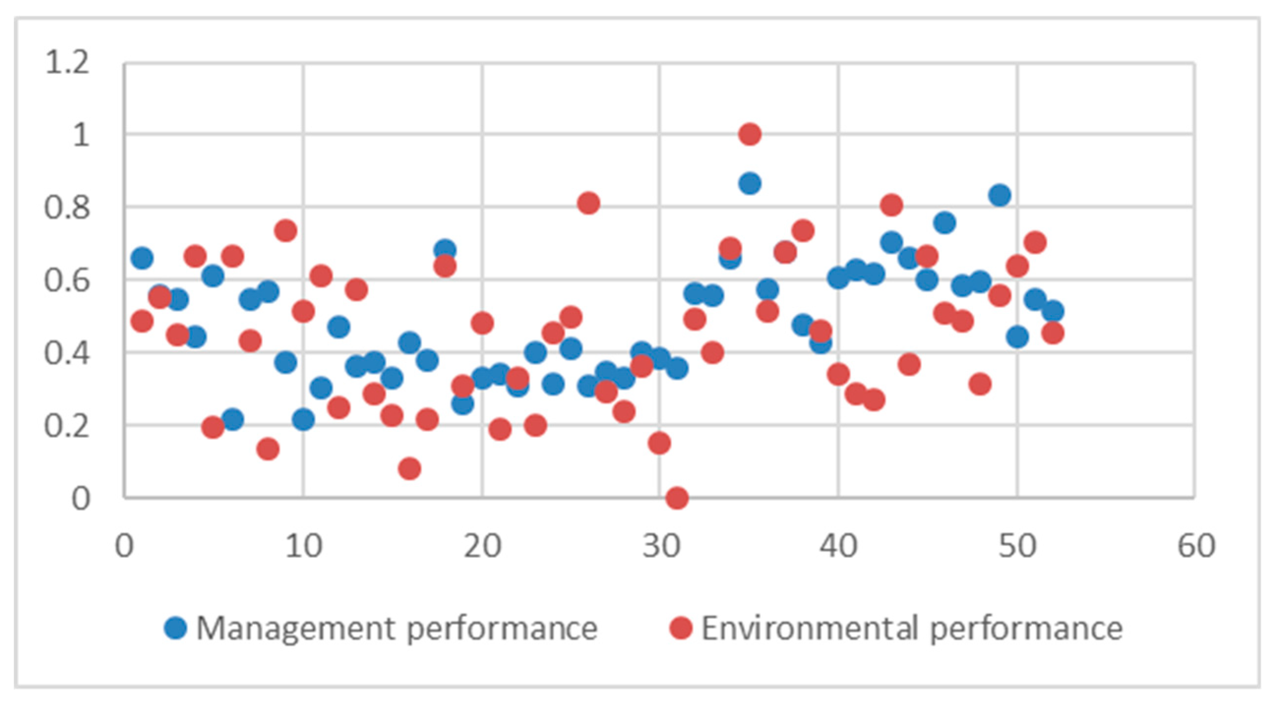
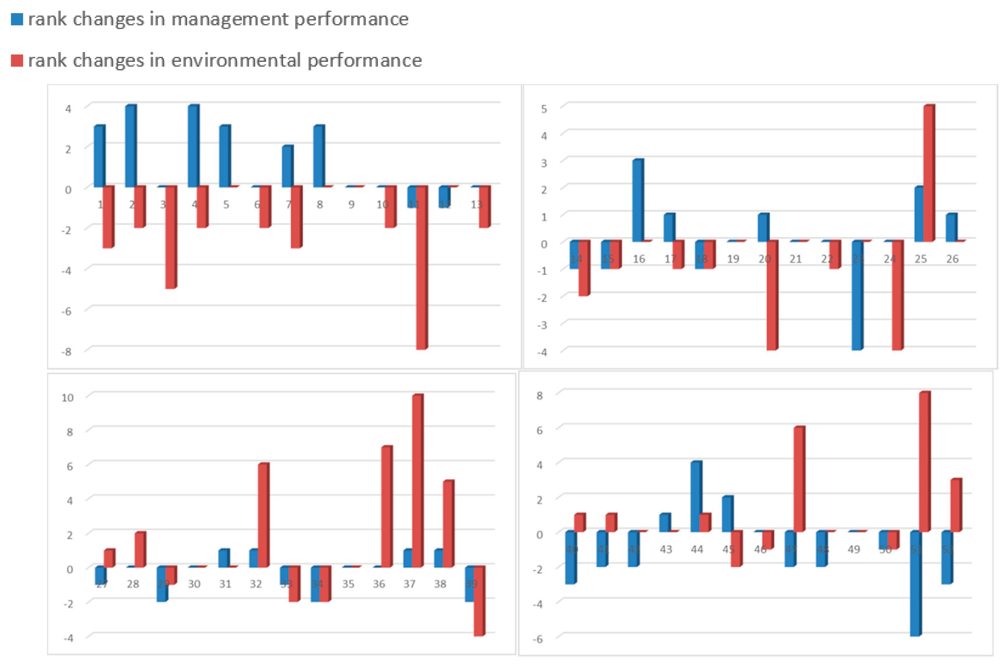
By analyzing all the family farms’ management and environmental performance, and by combining it with the information gathered from field research, several conclusions are drawn below.

a)

There is weak positive correlation between family farms’ management performance and environmental performance.

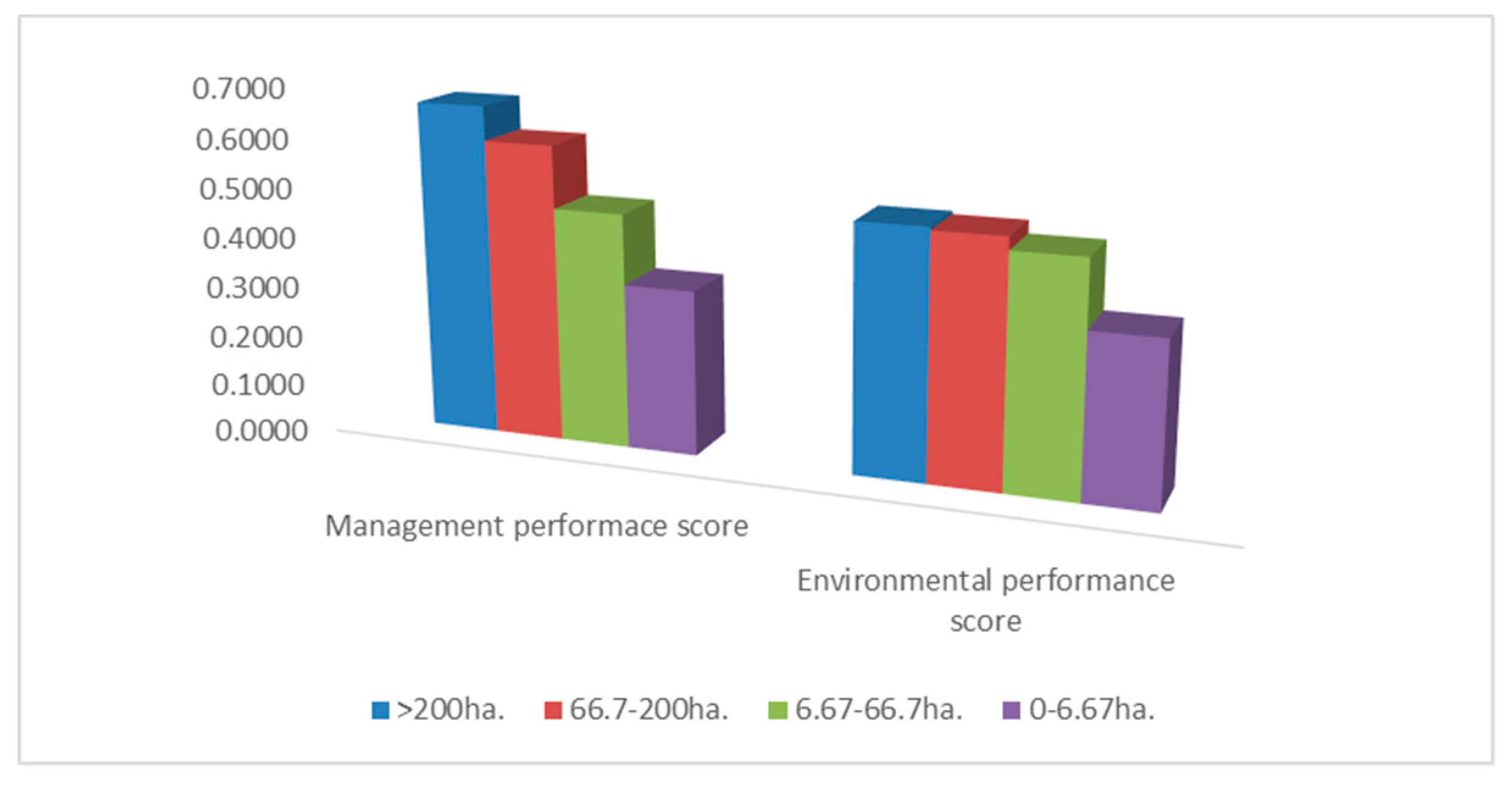
b)

There is a corresponding increase for all 52 selected family farms’ management and environmental performance with the expansion of utilized agricultural area. However, a higher variation extent for management performance than environmental performance is presented.

c)

According to the results of field research, farm owners’ management skills and experience play a great role in family farms’ daily operation. Farmers who are aware of the needs of environmental protection are usually those experienced farmers who have long-term plans for their family farm’s development.

d)

Based on the evaluation results of our selected family farms, we conclude that the number of crop species has an obvious impact on family farms’ management performance and family farms in Jilin province performed better than those of Shandong in 2017.

e)

The variables’ ranking order regarding their degree of influence on management performance is: labor wages, utilized agricultural area, land rent, machinery operation cost, fertilizer input, pesticide input, seed input, and crop output. There is an urgent demand for technological instruction for family farms, especially those that operate on a large scale. Farm owners need sufficient market information to make a decision about the production plan for the next year and improve agricultural production sales.

f)

The variables’ ranking order regarding their degree of influence on environmental performance is: fertilizer input per hectare, pesticide input per hectare, and straw recycling rate. New technology focusing on reducing the usage of fertilizer and pesticides should be introduced by the government. Meanwhile, laws that prohibit the burning of straw to avoid air pollution are urgently needed. Livestock breeding and mushroom cultivation can consume the straw and generate biological organic fertilizer.

Some limitations exist in this work. Firstly, we only collected the production data of 2017 rather than a time series data due to time constraint. Secondly, the sample size is relatively small and all the regional distribution is not wide enough. As future work, our research will pay attention to two aspects: (i) based on this research, time series data will be collected to conduct a trend analysis of family farm’s management and environmental performance and we would expand the sample size; and (ii) the proposed method UCCE will be applied in other fields, such as energy saving assessment and green evaluation. Moreover, software related to assessment methods will be designed and applied in the assessment process.

References

1. Li, H.; Dai, M.; Dai, S.; Dong, X. Current status and environment impact of direct straw return in China’s crop land-A review. Ecotoxicol. Environ. Saf. 2018, 159, 293–300. [Google Scholar] [CrossRef] [PubMed]
2. Huang, Z. Is “Family Farms” the Way to Develop Chinese Agriculture? Open Times 2014. [Google Scholar] [CrossRef]
3. Jiang, Y.; Qi, M. Formation mechanism, individual endowment and cultivation of family farmers. China Popul. Resour. Environ. 2018, 28, 170–176. [Google Scholar]
4. Gao, Q.; Zhou, Z.; Kong, X. Practice Definition, Qualification Conditions and Registration Management of Family Farms-Based on the Perspective of Policy Analysis. Issues Agric. Econ. 2014, 35, 11–18. [Google Scholar]
5. Graeub, B.E.; Chappell, M.J.; Wittman, H.; Ledermann, S.; Kerr, R.B.; Gemmill-Herren, B. The State of Family Farms in the World. World Dev. 2016, 87, 1–15. [Google Scholar] [CrossRef]
6. Family Farm Survey and Analysis—The Fourth Annual Report of Agricultural Economics Statistics in 2015. Rural. Manag. 2015, 10, 45. Available online: http://www.cnki.com.cn/Article/CJFDTotal-NCHZ201510028.htm (accessed on 17 December 2018).
7. Zhang, Y.; Liu, W. Productivity and Risk Analysis of Family Farms. Issues Agric. Econ. 2016, 37, 16–21. [Google Scholar]
8. Wang, S.; Zhang, C. Spatial and temporal distribution of air pollutant emissions from open burning of crop residues in China. Sci. Pap. Online 2008, 3, 329–333. [Google Scholar]
9. Chen, J.; Li, C.; Ristovski, Z.; Milic, A.; Gu, Y.; Islam, M.S.; Wang, S.; Hao, J.; Zhang, H.; He, C. A review of biomass burning: Emissions and impacts on air quality, health and climate in China. Sci. Total Environ. 2016, 579, 1000–1034. [Google Scholar] [CrossRef]
10. Zhou, Y.; Xing, X.; Lang, J.; Chen, D.; Cheng, S.; Wei, L.; Wei, X.; Liu, C. A comprehensive biomass burning emission inventory with high spatial and temporal resolution in China. Atmos. Chem. Phys. 2017, 17, 1–43. [Google Scholar] [CrossRef]
11. Zhang, L.; Li, X.; Yu, J.; Y, X. Toward Cleaner Production: What drives farmers to adopt eco-friendly agricultural production? J. Clean. Prod. 2018, 184, 550–558. [Google Scholar] [CrossRef]
12. Nicolopoulou-Stamati, P.; Maipas, S.; Kotampasi, C.; Stamatis, P.; Hens, L. Chemical pesticides and human health: The urgent need for a new concept in agriculture. Front. Public Health 2016, 4, 148. [Google Scholar] [CrossRef]
13. VoPham, T.; Bertrand, K.; Hart, J.; Laden, F.; Brook, M.; Yuan, J.; Talbott, E.; Ruddell, D.; Chang, C.; Weissfeld, J. Pesticide exposure and liver cancer: A review. Cancer Causes Control 2017, 28, 177–190. [Google Scholar] [CrossRef] [PubMed]
14. Brauns, B.; Jakobsen, R.; Song, X.; Bjerg, P.L. Pesticide use in the wheat-maize double cropping systems of the North China Plain: Assessment, field study, and implications. Sci. Total Environ. 2018, 616–617, 1307–1316. [Google Scholar] [CrossRef]
15. Charnes, A.; Cooper, W.W.; Rhodes, E. Measuring the efficiency of decision making units. Eur. J. Oper. Res. 1978, 2, 429–444. [Google Scholar] [CrossRef]
16. Doyle, J.; Green, R. Efficiency and cross-efficiency in DEA: Deviations, meanings and uses. J. Oper. Res. Soc. 1994, 45, 567–578. [Google Scholar] [CrossRef]
17. Farrell, M.J. The Measurement of Productive Efficiency. J. R. Stat. Soc. 1957, 120, 253–290. [Google Scholar] [CrossRef]
18. Essid, H.; Ganouati, J.; Vigeant, S. A Mean-Maverick Game Cross-Efficiency Approach to Portfolio Selection: An Application to Paris Stock Exchange. Expert Syst. Appl. 2018, 113, 161–185. [Google Scholar] [CrossRef]
19. Nikolaou, P.; Dimitriou, L. Evaluation of road safety policies performance across Europe: Results from benchmark analysis for a decade. Transp. Res. Part A Policy Pract. 2018, 116, 232–246. [Google Scholar] [CrossRef]
20. Yu, M.M.; Chen, L.H.; Hsiao, B. A performance-based subsidy allocation of ferry transportation: A data envelopment approach. Transp. Policy 2018, 68, 13–19. [Google Scholar] [CrossRef]
21. Despotis, D.K. Improving the discriminating power of DEA: Focus on globally efficient units. J. Oper. Res. Soc. 2002, 53, 314–323. [Google Scholar] [CrossRef]
22. Li, F.; Zhu, Q.; Chen, Z.; Xue, H. A balanced data envelopment analysis cross-efficiency evaluation approach. Expert Syst. Appl. 2018, 106, 154–168. [Google Scholar] [CrossRef]
23. Soleimani-damaneh, M.; Zarepisheh, M. Shannon’s entropy for combining the efficiency results of different DEA models: Method and application. Expert Syst. Appl. 2009, 36, 5146–5150. [Google Scholar] [CrossRef]
24. Song, L.; Liu, F. An improvement in DEA cross-efficiency aggregation based on the Shannon entropy. Int. Trans. Oper. Res. 2018, 25, 705–714. [Google Scholar] [CrossRef]
25. Wu, J.; Liang, L.; Yang, F. Determination of the weights for the ultimate cross efficiency using Shapley value in cooperative game. Expert Syst. Appl. 2009, 36, 872–876. [Google Scholar] [CrossRef]
26. Wu, J.; Sun, J.; Liang, L.; Zha, Y. Determination of the weights for the ultimate cross efficiency using Shannon entropy. Expert Syst. Appl. 2011, 38, 5162–5265. [Google Scholar] [CrossRef]
27. Wang, Y.M.; Wang, S. Approaches to determining the relative importance weights for cross-efficiency aggregation in data envelopment analysis. J. Oper. Res. Soc. 2013, 64, 60–69. [Google Scholar] [CrossRef]
28. Wu, J.; Sun, J.; Liang, L. DEA cross-efficiency aggregation method based upon Shannon entropy. Int. J. Prod. Res. 2012, 50, 6726–6736. [Google Scholar] [CrossRef]
29. Han, C. Individual Farmers and Scale Farming: Reviews of the Theoretics of the Family Farm. Econ. Res. J. 2017, 7, 184–199. [Google Scholar]
30. Zhang, C.; Huang, B.; Kong, X. Evaluation and Analysis of the Comprehensive Development Level of Family Farms-Taking the National Farming Family Farm as an Example. Jianghuai Trib. 2017, 3, 54–60. [Google Scholar]
31. Abay, C. An analysis of input use efficiency in tobacco production with respect to sustainability: The case study of Turkey. J. Sustain. Agric. 2004, 24, 123–143. [Google Scholar] [CrossRef]
32. Zhang, D.; Gong, T. The Technical Efficiency of Food Production in Linking Family Farms with Cooperatives. J. South China Agric. Univ. (Soc. Sci. Ed.) 2018, 17, 64–74. [Google Scholar]
33. Feng, S. Land rental, off-farm employment and technical efficiency of farm households in Jiangxi Province, China. NJAS-Wagening J. Life Sci. 2008, 55, 363–378. [Google Scholar] [CrossRef]
34. Uras, B.R.; Wang, P. Production Flexibility, Misallocation and Total Factor Productivity. Soc. Sci. Electron. Publ. 2017. [Google Scholar] [CrossRef]
35. Zhang, Z.; Zhang, Y.; Li, F.; Hui, Y.; Yuan, Y.; Yuan, X. Economic efficiency of small-scale tilapia farms in Guangxi, China. Aquac. Econ. Manag. 2016, 1–12. [Google Scholar] [CrossRef]
36. Zhu, Q.; Hu, P.; Xu, H. On Family Farms: Advantages, Conditions and Scale. Issues Agric. Econ. 2014, 35, 11–17. [Google Scholar]
37. Gao, Y.; Li, P. Factors affecting the growth of food family farms. J. South China Agric. Univ. (Soc. Sci. Ed.) 2017, 16, 1–11. [Google Scholar]
38. Gao, Y.; Zhang, X.; Wu, L.; Yin, S.; Lu, J. Resource basis, ecosystem and growth of grain family farm in China: Based on rough set theory and hierarchical linear model. Agric. Syst. 2017, 154, 157–167. [Google Scholar] [CrossRef]
39. Souza, G.D.S.E.; Gomes, E.G. Management of agricultural research centers in Brazil: A DEA application using a dynamic GMM approach. Eur. J. Oper. Res. 2015, 240, 819–824. [Google Scholar] [CrossRef]
40. Zhang, J.J.; He, P.; Xu, X.P.; Wang, Y.L. Nutrient Expert Improves Nitrogen Efficiency and Environmental Benefits for Summer Maize in China. Agron. J. 2017, 109. [Google Scholar] [CrossRef]
41. Fang, X.; Li, Y.; Nie, J.; Wang, C. Effects of nitrogen fertilizer and planting density on the leaf photosynthetic characteristics, agronomic traits and grain yield in common buckwheat (Fagopyrum esculentum M.). Field Crop. Res. 2018, 219, 169–179. [Google Scholar] [CrossRef]
42. Yang, L.; Huang, B.; Mao, M.; Yao, L.; Niedermann, S.; Hu, W.; Chen, Y. Sustainability assessment of greenhouse vegetable farming practices from environmental, economic, and socio-institutional perspectives in China. Environ. Sci. Pollut. Res. Int. 2016, 23, 17287–17297. [Google Scholar] [CrossRef] [PubMed]
43. Sun, J.; Peng, H.; Chen, J.; Wang, X.; Wei, M.; Li, W.; Yang, L.; Zhang, Q.; Wang, W.; Mellouki, A. An estimation of CO2, emission via agricultural crop residue open field burning in China from 1996 to 2013. J. Clean. Prod. 2016, 112, 2625–2631. [Google Scholar] [CrossRef]
44. Zeleny, M. Multiple Criteria Decision Making; McGraw-Hill: New York, NY, USA, 1982. [Google Scholar]
45. Sexton, T.R.; Silkman, R.H.; Hogan, A.J. Data envelopment analysis: Critique and extensions. In Measuring Efficiency: An Assessment of Data Envelopment Analysis; Silkman, R.H., Ed.; Jossey-Bass: San Francisco, CA, USA, 1986; pp. 73–105. [Google Scholar]
46. Hsu, C.-K.; Wang, C.-H.; Lee, C.-L.; Jou, C.-J. Use of Gray Relational Analysis to Manage and Optimize Full-Scale Industrial Furnace Operation. J. Hazard. Toxic Radioact. Waste 2018, 22, 04018026. [Google Scholar] [CrossRef]
47. Sylajakumari, P.A.; Ramakrishnasamy, R.; Palaniappan, G. Taguchi Grey Relational Analysis for Multi-Response Optimization of Wear in Co-Continuous Composite. Materials 2018, 11. [Google Scholar] [CrossRef]
48. Xu, F.; Zhang, S.; Wu, K.; Dong, Z. Multi-response optimization design of tailor-welded blank(TWB) thin-walled structures using Taguchi-based gray relational. Thin-walled Struct. 2018, 131, 286–296. [Google Scholar] [CrossRef]
49. Tseng, M.L.; Chiu, A.S.F. Evaluating firm’s green supply chain management in linguistic preferences. J. Clean. Prod. 2013, 40, 22–31. [Google Scholar] [CrossRef]
50. Deng, J.L. The introduction of grey system. J. Grey Syst. 1989, 1, 1–24. [Google Scholar]
51. Liu, W.; Qiu, L. Evaluation and Analysis on Scale Management of Family Farm Based on DEA Method. J. Agric. Mech. Res. 2009. Available online: http://www.cqvip.com/qk/97903x/2009012/32083058.html (accessed on 19 December 2018).
52. Oduol, J.B.A.; Hotta, K.; Shinkai, S.; Tsuji, M. Farm size and productive efficiency: Lessons from smallholder farms in Embu district, Kenya. J. Fac. Agric. Kyushu Univ. 2006, 51, 449–458. [Google Scholar]
53. Zhan, J.; Tian, X.; Zhang, Y.; Yang, X.; Qu, Z.; Tan, T. The Effects of Agricultural R&D on Chinese Agricultural Productivity Growth: New Evidence of Convergence and Implications for Agricultural R&D Policy. Can. J. Agric. Econ. /Rev. Can. Dagroeconomie 2017, 65. [Google Scholar] [CrossRef]
54. Cao, Y.; Du, Z.; Wan, G. Family farm’s choice of cropping behavior under different pesticide residue standards. Syst. Eng. -Theory Pract. 2018, 38, 1492–1501. [Google Scholar]
Figure 1. Cross-efficiency and relevant variables.
Sustainability 11 00006 g001
Figure 2. Ultimate management efficiency scores and CCR scores for 52 family farms.
Sustainability 11 00006 g002
Figure 3. Ultimate environmental efficiency scores and CCR scores for 52 family farms.
Sustainability 11 00006 g003
Figure 4. Ranking order changes of family farm performance.
Sustainability 11 00006 g004
Figure 5. Variation coefficients of the three approaches.
Sustainability 11 00006 g005
Figure 6. Scatter diagram of management and environmental efficiency scores.
Sustainability 11 00006 g006
Figure 7. Performance score in different scales.
Sustainability 11 00006 g007