Article

Nonlinear Dynamics in the Finance-Inequality Nexus in China-CHNS Data

by
Mohammad Masudur Rahman
1,2,
Guan Fuquan
3,* and
Laila Arjuman Ara
4
1
School of Business, Zhejiang University City College, Hangzhou 310015, China
2
Waikato Management School, The University of Waikato, Hamilton 3240, New Zealand
3
School of Economics and Management, Zhejiang A&F University, Hangzhou 311300, China
4
School of Business Studies, United International University, Dhaka 1210, Bangladesh
*
Author to whom correspondence should be addressed.
Sustainability 2019, 11(1), 191; https://doi.org/10.3390/su11010191
Submission received: 26 October 2018 / Revised: 18 December 2018 / Accepted: 27 December 2018 / Published: 2 January 2019
(This article belongs to the Section Economic and Business Aspects of Sustainability)

Abstract

:
This paper empirically investigates the effects of financial development on incomes of Chinese residents particularly within various income groups using data from six provinces by applying the Quantile Regression model. The Greenwood and Jovanovich hypothesis that illustrates the inverted U shaped relationship between financial development and income inequality is tested. This empirical study demonstrates that financial development has a positive but non-linear effect on the annual income of individuals from various income groups at different quantiles. The effect is an inverted U or Kuznets effect indicating an increase at first and then a drop. As for the distribution of the impact on various income groups, the low-income group is under the most dominant influence followed by the high-income group with the middle-income groups receiving relatively smaller influence. Findings indicate that promoting balanced financial development would help to ease the income gap between Chinese residents.
JEL Classification:
O150; O160; O180

1. Introduction

Income inequality is a widespread concern around the world, especially in developing countries. Former US President Barak Obama even called the widening income inequality the “defining challenge of our time” [1]. Income inequality has increased globally, but there is no consensus yet about its causes. In the recent literature, the impact of finance on income inequality has been getting huge attention globally. However, there are conflicting views about the relationship between finance and income inequality. Financial development (FD) refers to an increase in the volume of financial activities, and is mostly measured by credit to the private sector relative to the Gross Domestic Product (GDP) [2].
It is well known that financial development plays a positive role in economic development, but there are no generalized conclusions on whether financial development can reduce income inequalities. Kuznets [3] hypothesized on the relationship between economic growth and the distribution of income. Kuznets cautiously offered the proposition that during the course of an economy’s lifetime, income inequality rises during the early stage of development, tapers off during the juvenile stage, and finally declines as the market reaches maturity level. Due to fixed costs that are not affordable by everyone, usually the poor cannot access financial services at the primary stage of economic growth. Nevertheless, they will keep their savings, hoping to step across the threshold level of wealth someday and become investors with support from the financial market. Financial institutions typically provide services to the high-end customers. These financial services obviously benefit the high-income group by increasing their incomes and thereby increasing income inequalities. With the economy and financial sector becoming more developed and mature, an increasing number of poor people can cross the threshold of wealth to access financial services. When most people can receive investment returns via the financial market, financial development may reduce income inequalities.
The Chinese economy has been growing dramatically, and real income of its residents has increased remarkably over the decades. Concurrently, the income distribution gap has been widening. Data released by the National Bureau of Statistics (NBS) shows that the Chinese Gini coefficient was only 0.16 in 1978, peaked at 0.491 in 2008, and then decreased to 0.469 in 2014. However, it has remained above the international caveat level of 0.47 over the present decade [4]. The research group in the Social Development Institute (SDI) of the National Development and Reform Commission (NDRC) [5] has pointed out that Chinese income inequality is higher than developed and most developing countries. According to studies in the first Blue Book of Social Administration [6], one of the most critical factors transforming potential risks into public crises is the broadening income gap between the rich and the poor.
There are various studies showing that financial development reduces income inequalities [7,8,9,10,11,12,13]. Numerous studies have investigated the Kuznets curve on financial development and income inequalities and confirmed the Kuznets curve that means that financial development initially increases income inequality, but this inequality decreases after a certain period. Burgess and Rohini [10] found that licensing regulations imposed by the Indian Government on commercial banks led to an increase in the number of agencies set up in rural areas by many commercial banks. This policy significantly reduced the urban–rural income gap in a selected area of India. With cross-country panel data Beck et al. [9] found that financial development could lower the Gini coefficient. Shahbaz and Islam [14] and Batuo et al. [15] found that financial development has a significantly positive impact on reducing income inequality.
However, under certain conditions, particularly an imperfect finance market, financial development may hinder and may widen the income gap [16,17,18]. de Hann and Strum [16] examine how financial development, financial liberalization, and banking crises are related to income inequality and suggest that all finance variables increase income inequality. Galor and Zeira [17] and Banerjee and Newman [18] believe that with the imperfect financial markets, financial and economic development will increase the income gap. Clarke et al. [11] found that financial development could help decrease the Gini coefficient if financial development made it easier for laborers to enter modern industrial sectors although they did not confirm the Kuznets curve. Arora [19] points out that the development of the financial system can worsen the income distribution. Kim and Lin [20], Tan and Law [21], Zhang and Chen [22] and Shahbaz et al. [14] provide some evidence for the non-linear hypothesis proposed by Greenwood and Jovanovic [7]. Hoi and Hoi [12] investigate the relationship between financial sector development and income inequality in Vietnam using provincial-level data and find that financial sector development has a positive impact on reducing income inequality; but no evidence to support the Greenwood–Jovanovic [7] hypothesis of an inverted U-shaped relationship between the development of the financial sector and income inequality.
In China, income inequalities are represented by income differences mostly between rural and urban areas. Though, there are various empirical studies focused on the influence of financial development on the urban–rural income gap, the literature shows that the relationship between financial development and income inequalities are inconclusive and mixed. Some have found more developed finance broadens the income gap [22,23,24]; whereas others think that, the relationship between financial development and income inequalities may confirm the Kuznets hypothesis [22,25,26].
Zhang and Chen [22] explored the relationship of financial development and income inequality in China using structural vector auto-regression. The empirical results are consistent with the hypothesis of having an inverted U-shaped relationship between financial development and income inequality. Liu et al. [26] investigated the impacts of financial development and income inequality in different administrative districts (urban, rural and overall) in China using a dynamic generalized method of moments estimator and provided some evidence for a linear and inverse ‘U-shape’ relationship between financial development and income inequality.
The above brief review shows that most of the studies on financial development and income gap data collected from various regions and findings are indecisive. Most of the studies on the Chinese economy are based on macro perspectives; however, few studies are devised from a micro view with a small dataset. Against this backdrop, this paper empirically investigates the effect of financial development on incomes of residents particularly within various income groups using the large sample conducted by the China Health and Nutrition Survey (CHNS) of Chinese residents of six provinces and autonomous regions. We used quantile regression to estimate the effect of the financial development which is a new attempt in the literature. The quantile regression can capture the nonlinearity effect in different levels of quantile [27]. In the next section, we describe the empirical model and the data used. The empirical analysis is presented in Section 3 with Section 4 offering conclusions.

2. Methodology and Data

2.1. Empirical Model

The Quantile regression [27] model has been adopted in this paper to test the influence of financial development on the income of Chinese residents. Compared with mean regression, this is not restricted to the hypothesis that the error term should follow a normal distribution and can more accurately describe the various effects of independent variables on the dependent variable in different sections; thus, steadier and comprehensive analysis results can be found using quantile regression analysis [27]. Specifically, the following quantile regression model has been adopted to study the influence of financial development on incomes of residents:
y = α 0 + α 1 F D + α 2 F D 2 + β X + ε
where y is the natural logarithm of the annual incomes for residents; F D is the financial development index which is composed of the total loan of financial institutions divided by GDP, thereby representing financial development levels in various regions; and F D 2 is the quadratic term of the financial development indicator used to test the non-linear effect. Also, X represents a series of explanatory variables that can affect incomes of residents including gender, age, educational level, marital status, residency, a time dummy variable, and provincial dummy variables.
To realize the heterogeneous effect of these factors on the financial development of residents with different income groups as proposed by Koenker [27], a quantile regression was applied to each quantile of y in Equation (1). The conditional quantile of y that is distributed in p can then be presented as follows:
q p ( y | F D , F D 2 , X ) = α 0 ( p ) + α 1 ( p ) F D + α 2 ( p ) F D 2 + β ( p ) X + ε ( p )
Because no hypothesis on the distribution of the random disturbance term should be made in quantile regression, the quantile estimates can be computed through the minimized sum of the absolute value of the residual error in Equation (2).

2.2. Data Variables

For Detailed Questionnaire and Structure of the survey Data and Variables, Please Visit—http://www.cpc.unc.edu/projects/china.
The samples selected for the empirical study are from five provinces (Shandong, Henan, Jiangsu, Hubei, and Hunan) and one autonomous region (Guangxi Zhuang Autonomous Region) where financial development and income distribution of its residents are distinctive and representative. Until 2015, the CHNS covered 15 provinces of the survey. As the income and financial development of the three mega cities that is Beijing, Shanghai, and Chongqing are much higher than the other provinces which are not compatible, we omitted these mega cities from our study. The three-mega cities survey was conducted in 2011 therefore a time series database was also not available. On the other hands another three provinces Shaanxi, Yunnan, and Zhejiang were added in the database also only in 2015 and therefore no time series data was available. Data, from the China Health and Nutrition Survey (CHNS) (China Health and Nutrition Survey (CHNS), Carolina Population Center, University of North Carolina, Chapel Hill, http://www.cpc.unc.edu/projects/china), were collected which is a joint effort of the Demographic Research Center of the University of North Carolina and the Chinese Center for Disease Control and Prevention [28]. The data were collected for 2000, 2004, 2006, 2009, and 2011, including personal features, family characteristics, and incomes. Gross Domestic Product (GDP), loan, and population data were collected from various statistical yearbooks of different Provinces and Autonomous Regions. Other financial development indicators were also used, such as branches of commercial banks and cooperative unions per capita that was compiled from various statistical yearbooks of banks and rural cooperative unions statistical years books. The total volume of the sample is 18,954, aged from 18 to 65. The personal annual incomes of residents are taken as the dependent variable to measure earnings. According to data instructions provided by CHNS, personal annual income includes wages and operating incomes. Individual income is conceptualized as the sum of all sources of income and revenue minus expenditures for one resident [28]. It is not a simple division of a resident’s income evenly divided among resident members (that is per capita income, which is computed as part of a resident’s income). Rather, individual income is built by adding each person’s income source. There were questions about seven potential sources of income in the questionnaires: business, farming, fishing, gardening, livestock, non-retirement wages, and retirement income. After calculating individual income from each source, total individual income was constructed as the sum from all seven sources (Individual Income Variable Construction, CHNS).
Income data were adjusted to the price level in 2006 based on the Consumer Price Index (CPI). The ratio of outstanding loans to GDP was used to measure the level of financial development (FD)of different regions in different years. With reference to the research by Arestis, Panicos, and Demetriades [29], Qiao and Li [25], Sun and Yulin [23], Wan and Shi [24], and Yuan et al. [30], due to the obvious bank-dominated financial structure in China, it was relatively reasonable to use these indicators to measure the degree of financial development. As the districts level loan outstanding data was not available, details of the total outstanding loans and GDP of all six provinces and autonomous regions over five years were collected. Therefore, dummy variables including age, level of education, gender (male = 1, female = 0), marital status (married = 1, unmarried = 0), and residence (urban/non-agricultural registered permanent residence = 1, agricultural registered permanent residence = 0) were used. Moreover, time and provincial dummy variables were used to control time and regional differences. Besides, the number of branches per capita was used as another financial indicator to check the robustness of the financial indicators. Consideration was only given to the number of branches of commercial banks and rural cooperatives unions. Finally, the number of branches was converted to per capita branches by dividing by the population of the respective provinces.

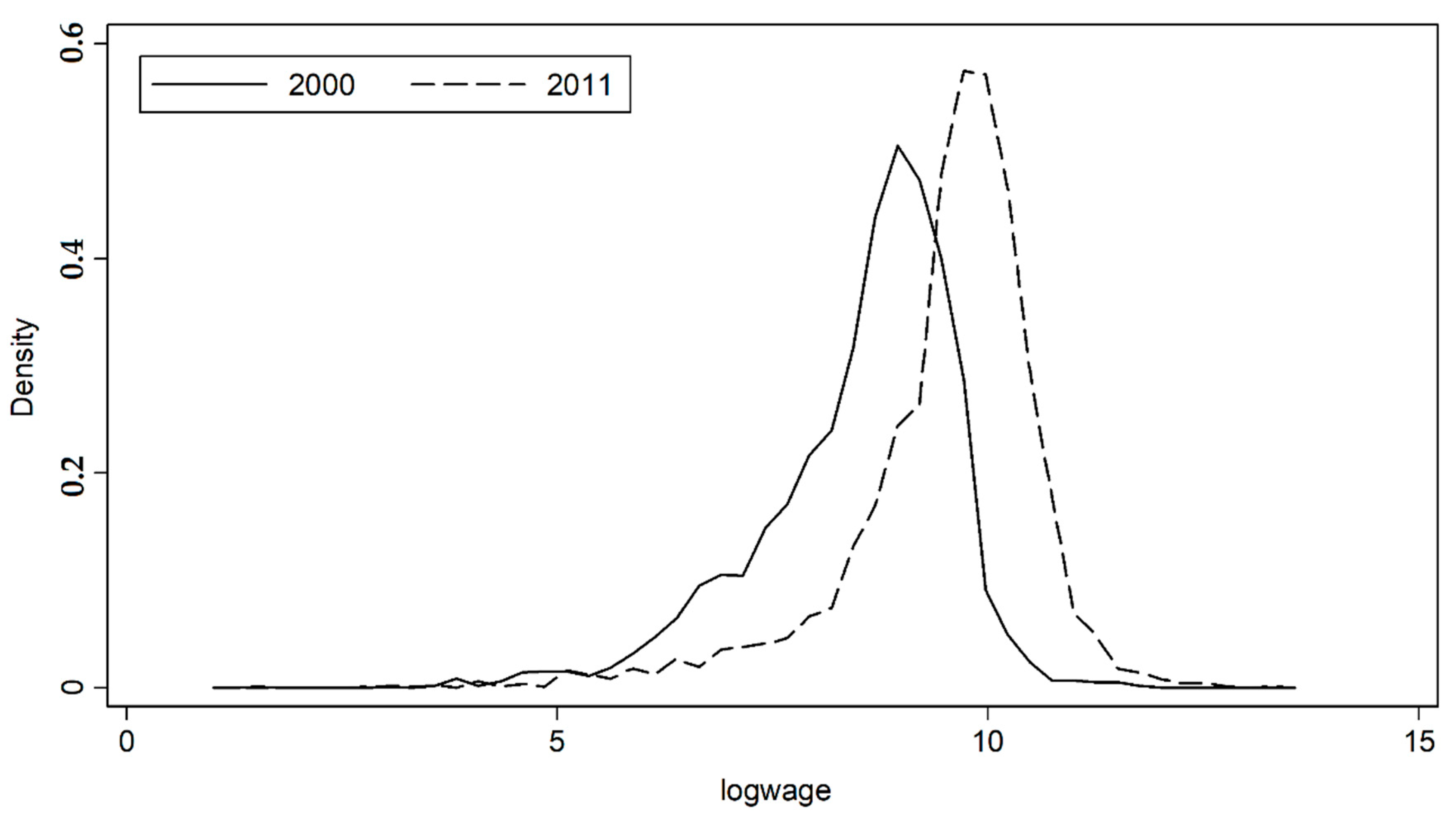
2.3. Descriptive Statistics

Figure 1, shows the kernel density diagram of the logarithm of annual incomes of 2000 and 2011 (Epanechnikov kernel function is adopted). During this period, average annual income (logarithmic value) increased by 11.29 percent, which makes income distribution improve as a whole. The annual income of the two low-income groups increased in income distribution (17.56 percent for the group located at quantile 0.1 and 13.48 percent for quantile 0.25), which were both higher than average growth. Meanwhile, the annual income of the high-income groups increased (located at quantile 0.75, increased by 9.21 percent and quantile 0.9 increased by 9.46 percent) but was lower than average.
In 2000, the income ratio for quantiles 0.25 and 0.1 was at the bottom of the income distribution which was 1.14, and in 2011, this ratio decreased to 1.10 indicating a narrowing of the income gap. However, the income ratio for quantiles 0.9 and 0.75 was at the top of income distribution, which was 1.04 both in 2000 and 2011 meaning the income gap did not grow wider. This demonstrated that income inequalities were less severe in 2011 than in 2000, mainly represented by the narrowing of the income gap of the low-income groups and the higher-than-average increase of their incomes. From Figure 1, it can be perceived that income distribution, even with a logarithmic transformation, was evident with asymmetry and skewness. This non-normality proved that if estimates were calculated by a traditional ordinary least-squares (OLS) regression method, the results would not be efficient.
Table 1 shows the descriptive statistics of economic and financial information for the sample dataset. In the samples, the average annual income of residents reaches RMB 14,694 with annual incomes as follows: the low-income group (an annual income below quantile 0.25) was RMB 2257, the middle-income group (an annual income between quantile 0.25 and quantile 0.75) was RMB 10,408, and the high-income group (an annual income above quantile 0.75) was RMB 35,684.
It is also deduced from Table 1 that the low-income group consists of people living in a place where the financial development index is lower, people are comparatively older and less educated, and there is a larger proportion of females and people with a rural registered permanent residence. In terms of regional distribution, Henan Province has the largest share of the low-income group, while Jiangsu Province has the largest proportion of the high-income group.

3. Findings: Quantile Regression Analysis

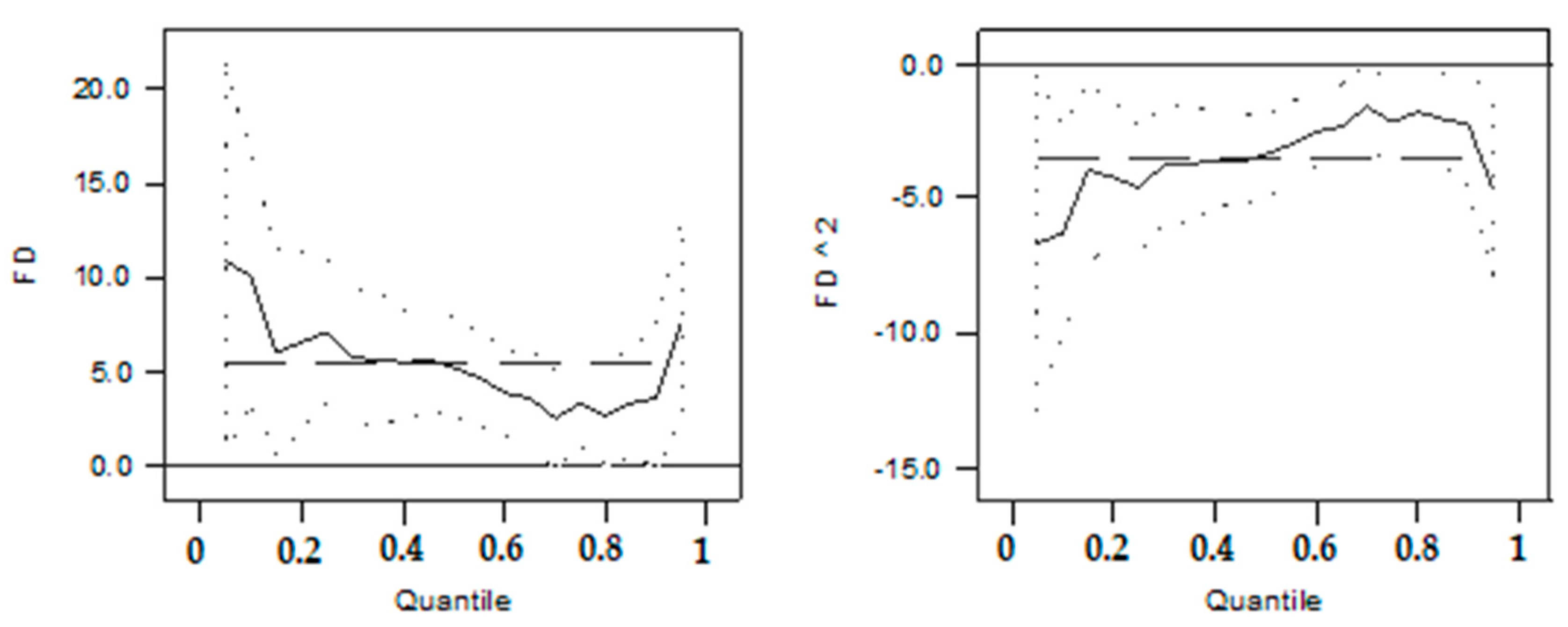
3.1. Results of Quantile Regression

Five quantiles on income distribution are chosen for this analysis. As listed in order, these are quantiles 0.05, 0.25, 0.5, 0.75, and 0.95. The regression results of quantile models are shown in Table 2. In these models, the provincial fixed effect (for Jiangsu, Shandong, Henan, Hubei, and Hunan Provinces as well as Guangxi Province, among which Jiangsu Province is the reference group) and the time fixed effect (for 2000, 2004, 2006, 2009, and 2011, with 2000 as the reference group) are controlled. OLS regression results are also presented to compare the difference in results of this traditional regression and the Quantile regression.
As the results indicate with variables of gender, marital status, residence, educational level, age, and provincial as well as time fixed effects being controlled, the level of financial development has a significant effect on individual annual incomes. With regional loan size/GDP and its quadratic term as the gauge of financial development, the coefficient estimates of the regression model at various quantiles are both positive and negative and most of them are significant at the 1 percent level. Another financial development indicator i.e., branch/population was also used to run a quantile regression to check robustness. The number of branches of commercial banks and rural cooperatives banks were collection from various Chinese Statistical Yearbooks. Similar results were found from this indicator as well and results are presented in the Appendix A (Table A1).
Different from most of the studies in China that are focused on analyzing the relationship between financial development and income gap, particularly the urban–rural income gap, this empirical study directly analyses the relationship between financial development and individual incomes. It turns out that for all of the residents from various income groups, financial development has a positive but non-linear effect on their personal incomes. This finding further demonstrates that financial development is a critical variable and plays a distinctive role in determining individual incomes in China.

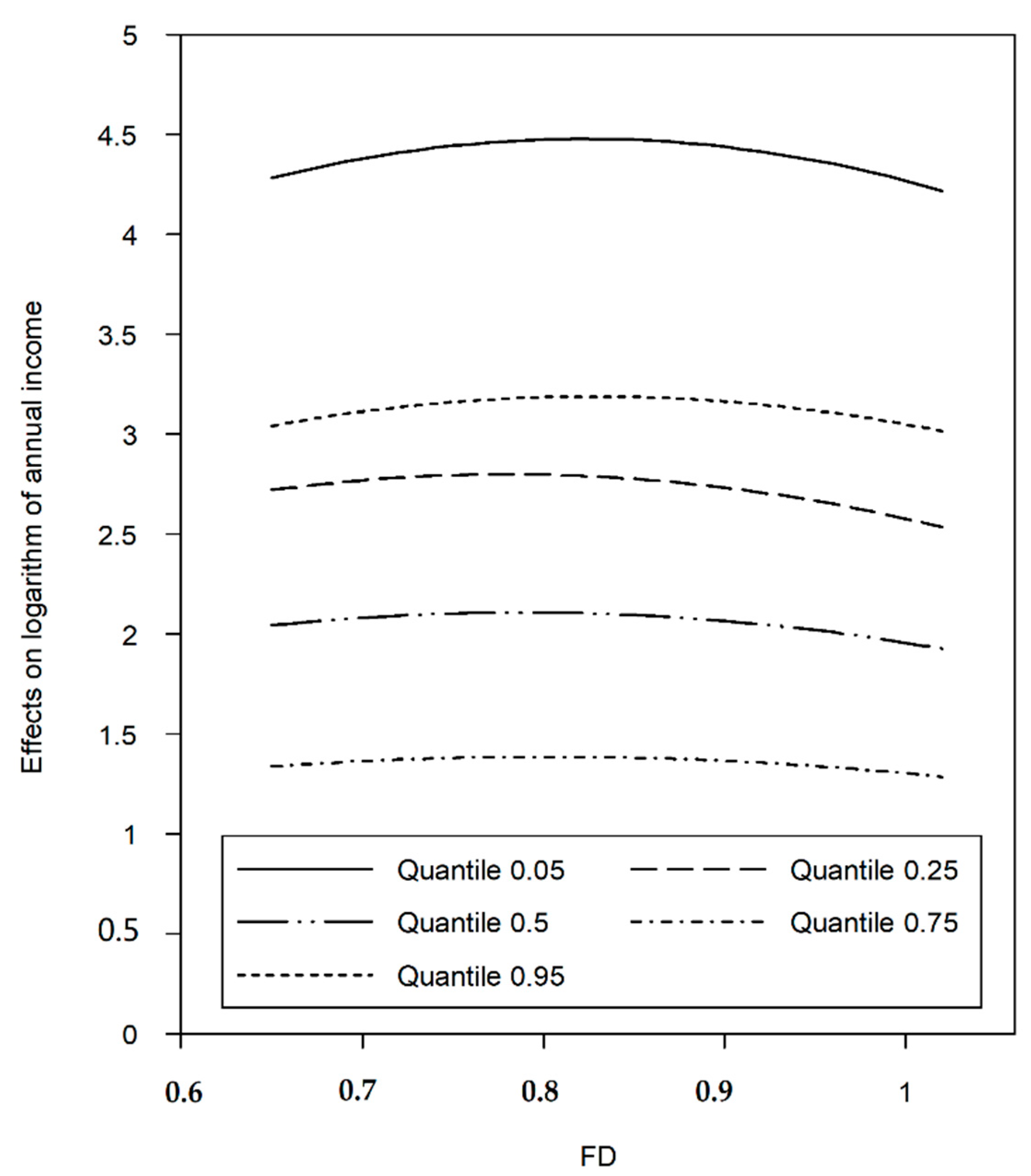
3.2. Effects of Financial Development(FD) on Various Income Groups

Figure 2 presents the effect of F D and F D 2 on annual income distribution. The solid lines estimate various quantiles, while dotted lines correspond to 95 percent confidence intervals.
For the convenience of contrast, the mean effect estimates of OLS are described through the dashed line. With the help of the regression results from Table 2, it is easy to find that financial development plays a different role in the incomes of low, middle, and high-income groups. This distinctive feature cannot be found by using OLS regression. The results also indicate a functional relationship between financial development and annual income.
The influences of FD and FD2 on annual income distribution are respectively in the left and right graphs. The solid line represents the effect of FD variables on various quantiles in income distribution. The dotted line is for the 95 percent confidence intervals in correspondence. To make it easier for comparison, the mean effect from OLS regression is described by the long dashed line.
As indicated in Figure 3, financial development is generally supportive for improving incomes of Chinese residents. The effect confirms the Kuznets effect or inverted U, showing that regional financial development has a positive but non-linear effect on incomes, increasing at first and then decreasing. Thus, this could help to achieve the prosperity for Chinese residents in these regions.
Among residents with different incomes, the low-income group at quantile 0.05 enjoys the greatest benefits (shown by the solid line in the Figure 3) and then the high-income group follows at quantile 0.95 (indicated by the short-dashed line in Figure 3). The middle-income groups at quantile 0.5 and quantile 0.75 are under relatively small influence (shown by dotted-long dashed line and dotted-short dashed line in Figure 3). This means that financial development, on the one hand, can help curb the income gap of the low-income groups, but on the other hand it can broaden the gap between the high-income group and other groups.
Our findings are compatible with the findings of Caravire and Rioja [31] as the Chinese economy has already crossed a certain level of financial development. Caravire and Rioja [31] found that financial development reduced overall income inequality in Latin America and the Caribbean (LAC) although the poorest quantile was not affected much by expansion in the financial sector. Nevertheless, they found some evidence for the Greenwood–Jovanovic [7] hypothesis that has a positive effect only after a country crosses a certain economic development. Although, Jorge [32] concludes that due to the imperfect nature of the Latin American market it is hard to find any direct link between the financial development and income inequality.
Financial development plays a significant role in promoting the income of the low-income group. This means that with the help of government policies, financial development has made a difference regarding creating essential financial services and curbing financial exclusion of the low-income group. According to Table 1, China’s low-income groups are mainly in rural areas. This indicates that equalization of financial services in urban and rural areas has been enhanced. From the perspective of a realistic economy, the Chinese Government has been paying attention to enhancing rural finance and services over the decades. Particularly, great importance has been attached to the central role of rural banking and rural credit cooperatives in strengthening the rural economy. By the end of 2015, 778,700 rural credit cooperatives had been established nationwide, and they have had an enormous impact on rural financing and business (NSB 2016). The financial services, capabilities, and effectiveness of the Agricultural Bank of China improved dramatically in rural areas. Besides, the rapid development of new rural financial institutions, particularly of rural community banks and loan companies, has expanded services in agricultural and rural areas. There were 876 rural community banks and 6080 microfinance companies nationwide in 2015 (NSB 2016). The loan size of those with rural registered permanent residence increased at a rate of 22.3 percent over the last five years, which is much higher than the national average for loans.
To draw a robustness check we also use the number of branches in addition to provincial loans (scaled by GDP). The provincial fixed effects are included in the empirical model to control the variation of loans of temporal change from year to year within each province. However, because increasing personal income can induce financial development, reverse causality may be concerned. Therefore appropriate instrumental variables (IV) would have been useful for robustness analysis. However, as long as the provincial level amount of loans to be instrumented is provincial-level macro variable and CHNS data do not contain individual-level micro financial information, finding appropriate instrumental variables in the current combination of data sets is difficult.

4. Conclusions

China’s economy is developing impressively; however, a severe problem on income distribution is emerging. The Greenwood and Jovanovich [7] hypothesis illustrates as income levels rise, the financial structure becomes more extensive, economic growth becomes more rapid, and income inequality across the rich and poor widens. In maturity, an economy has a fully developed financial structure, attains a stable distribution of income across the people, and has a higher growth rate than in its infancy.
Against this backdrop, this paper empirically investigated the effect of financial development on incomes of residents, particularly within various income groups, using a large sample of Chinese residents from six provinces applying the quantile regression model. The Greenwood and Jovanovich [7] hypothesis which illustrates the inverted-U shaped relationship between financial development and income inequality was tested. The provincial fixed effect (for Jiangsu, Shandong, Henan, Hubei, and Hunan Provinces as well as Guangxi Province, among which Jiangsu Province was the reference group) and the time fixed effect (for 2000, 2004, 2006, 2009, and 2011, with 2000 as the reference group) were controlled. Incomes of different income groups were found to be influenced by financial development. With personal characteristics and regional variables controlled, at various quantiles the coefficient estimates of financial growth were positive, and their quadratic terms negative. This indicates that financial development has a positive, but non-linear effect on the income of all different groups of residents.
The results also confirm a functional relationship between financial development and the logarithm of annual incomes at various quantiles. In addition, the results indicate that financial development could help raise the overall incomes of Chinese residents, and the effect is of an inverted U or Kuznets effect where the influence of regional financial development on income growth grew larger at first and then smaller. Moreover, given residents from different income groups, the low-income group enjoyed the most significant benefits, followed by the high-income group with the middle-income group experiencing a relatively smaller influence. This signifies that there are differences in the impact of financial development on various income groups.
The above conclusions have some policy implications. First, as finance is at the center of the modern economy, financial resources and services play a significant role in the reallocation of resources; therefore, it is necessary to implement policies to promote balanced financial development so that all citizens can reasonably enjoy financial services and the fruit of economic growth. Financial development has an incredible marginal effect on enhancing the income of low-income groups. Thus, it is essential to support rural financing to increase the income of low-income groups, particularly in rural areas.

Author Contributions

M.M.R., G.F. and L.A.A. contributed equally on this article.

Funding

This research was founded by the Natural Science Foundation of Zhejiang Province, China (Fund No. LY15G030032.

Acknowledgments

The earlier version of this paper was presented at the Asian Growth Research Institute (AGI), Kitakyushu, Japan on 6 September 2016 when the first author was a Visiting Fellow at AGI. We would like particularly to thank Charles Yuji Horioka, Eric D. Ramstetter, Tatsuo Hatta, Yoko Niimi and Dai Er-Biao of the AGI for their valuable comments and suggestions.

Conflicts of Interest

The authors declare no conflict of interests.

Appendix A

Table A1. Regression Results Using No. of Branches/Population as Financial Indicator.
Dependent Variables: Log (Branch/Population)OLSQuantile
0.050.250.50.750.95
FD2.235 **5.453 **4.773 ***3.234 **2.232 **5.012 **
(1.023)(2.048)(1.065)(1.121)(1.012)(1.903)
FD2−1.821 **−4.231 **−3.123 **−2.591 **−1.989 **−4.221 ***
(0.708)(2.001)(1.131)(1.013)(0.901)(1.223)
Male0.179 *0.0740.212 *0.211 **0.176 *0.241 **
(0.089)(0.038)(0.077)(0.069)(0.074)(0.060)
Married0.331 ***0.133 *0.126 **0.106 **0.081 **0.125 **
(0.074)(0.064)(0.030)(0.027)(0.020)(0.038)
Urban registered permanent residence0.212 ***0.539 ***0.335 **0.501 **0.153 ***0.112 ***
(0.036)(0.072)(0.033)(0.025)(0.020)(0.028)
Length of education0.076 ***0.128 ***0.089 **0.071 **0.054 ***0.043 ***
(0.002)(0.007)(0.003)(0.002)(0.002)(0.004)
Age0.0010.009−0.0040.004−0.002−0.005
(0.001)(0.008)(0.004)(0.007)(0.002)(0.013)
Provincial fixed effectYesYesYesYesYesYes
Time fixed effectYesYesYesYesYesYes
Sample size18,95418,95418,95418,95418,95418,954
Source: Authors Calculations. Note: ***, **, * denote statistical significance at the 1, 5, and 10 percent levels. The value in parentheses is the standard error.

References

  1. Dabla-Norris, E.; Kochhar, K.; Ricka, F.; Suphaphiphat, N.; Tsounta, E. Causes and Consequences of Income Inequality: A Global Perspective; IMF Staff Discussion Note 15/13; IMF: Washington, DC, USA, 2015. [Google Scholar]
  2. Abiad, A.; Detragiache, E.; Tressel, T. A New Database of Financial Reforms. IMF Econ. Rev. 2010, 57, 281–302. [Google Scholar] [CrossRef]
  3. Kuznets, S. Economic Growth and Income Inequality. Am. Econ. Rev. 1955, 45, 1–28. [Google Scholar]
  4. National Bureau of Statistics (Various Years), The People’s Republic of China, Various Issue. Available online: http://www.stats.gov.cn/ (accessed on 9 October 2016).
  5. Institute of the National Development and Reform Commission. Study on the Income gap of Residents in China; National Development and Reform Commission, Economic Research Reference: Beijing, China, 2012; Volume 25, pp. 3–23.
  6. Li, Y. Blue Book of Social Administration; Chinese Academy for Social Sciences (CASS): Beijing, China, 2012.
  7. Greenwood, J.; Jovanovich, B. Financial Development, Growth, and the Distribution of Income. J. Political Econ. 1990, 98, 1076–1107. [Google Scholar] [CrossRef] [Green Version]
  8. Sebastian, J.; Watzka, S. Financial Development and Income Inequality, CESifo Working Paper: Fiscal Policy, Macroeconomics and Growth, No. 3687. 2011. Available online: http://www.econstor.eu/bitstream/10419/55340/1/685220540.pdf (accessed on 9 December 2016).
  9. Beck, T.; Asli, D.; Levine, R. Finance, Inequality, and Poverty: Cross-Country Evidence; NBER Working Paper 10979; The World Bank: Washington, DC, USA, 2004. [Google Scholar]
  10. Burgess, R.; Rohini, P. Do Rural Banks Matter? Evidence from the Indian Social Banking Experiment. Am. Econ. Rev. 2005, 95, 780–795. [Google Scholar] [CrossRef] [Green Version]
  11. Clarke, G.; Lixin, C.X.; Heng, Z. Finance and Income Inequality: Test of Alternative Theories; Policy Research Working Paper; No. 2984; The World Bank: Washington, DC, USA, 2003. [Google Scholar]
  12. Hoi, L.Q.; Hoi, C.M. Financial Sector Development and Income Inequality in Vietnam: Evidence at the Provincial Level. J. Southeast Asian Econ. 2013, 30, 263–277. [Google Scholar] [CrossRef]
  13. Kaidi, N.; Sami, M. Financial Development and Income Inequality: The Linear versus the Nonlinear Hypothesis. Econ. Bull. 2016, 36, 609–626. [Google Scholar]
  14. Shahbaz, M.; Islam, F. Financial Development and Income Inequality in Pakistan: An Application of ARDL Approach. J. Econ. Dev. 2011, 36, 35–58. [Google Scholar]
  15. Batuo, M.E.; Guidi, F.; Mlambo, K. Financial Development and Income Inequality: Evidence from African Countries; Working Paper; University of Westminster: London, UK, 2014. [Google Scholar]
  16. de Hann, J.; Strum, J. Finance and income inequality: A review and new evidence. Eur. J. Political Econ. 2017, 50, 171–195. [Google Scholar] [CrossRef] [Green Version]
  17. Galor, O.; Joseph, Z. Income Distribution and Macroeconomics. Rev. Econ. Stud. 1993, 60, 35–52. [Google Scholar] [CrossRef]
  18. Banerjee, A.V.; Andrew, F.N. Occupational Choice and the Process of Development. J. Political Econ. 1993, 101, 274–298. [Google Scholar] [CrossRef]
  19. Arora, R.U. Finance and Inequality: A Study of Indian States. Appl. Econ. 2012, 44, 4527–4538. [Google Scholar] [CrossRef]
  20. Kim, D.H.; Lin, S.C. Nonlinearity in the Financial Development-income Inequality Nexus. J. Comp. Econ. 2011, 39, 310–325. [Google Scholar] [CrossRef]
  21. Tan, H.B.; Law, S.K. Nonlinear Dynamics of the Finance-inequality Nexus in Developing Countries. J. Econ. Inequal. 2012, 10, 551–563. [Google Scholar] [CrossRef]
  22. Zhang, Q.; Chen, R. Financial Development and Income Inequality in China: An Application of SVAR Approach. Procedia Comput. Sci. 2015, 55, 774–781. [Google Scholar] [CrossRef] [Green Version]
  23. Sun, Y.; Wan, Y. Financial development, opening-up, and urban-rural income gap. J. Financ. Res. 2011, 1, 28–39. [Google Scholar]
  24. Wan, H.; Shi, L. The impact of residents’ residence discrimination on urban-rural income gap. Econ. Res. J. 2014, 9, 43–55. [Google Scholar]
  25. Qiao, H.; Li, C. Re-examination of the “inverted U-shaped” relationship between financial development and income gap. Chin. Rural Econ. 2009, 7, 68–76. [Google Scholar]
  26. Liu, G.; Liu, Y.; Zhang, C. Financial Development, Financial Structure and Income Inequality in China. World Econ. 2017, 40, 1890–1917. [Google Scholar] [CrossRef]
  27. Koenker, R. Quantile Regression; Cambridge University Press: Cambridge, UK, 2005. [Google Scholar]
  28. Carolina Population Center. China Health and Nutrition Survey (CHNS); Carolina Population Center, University of North Carolina: Chapel Hill, NA, USA, 2014; Available online: http://www.cpc.unc.edu/projects/china (accessed on 19 October 2016).
  29. Arestis, P.; Panicos, O.; Demetriades, K.B. Financial Development and Economic Growth: Role of Stock Markets. J. Money Credit Bank. 2001, 33, 16–41. [Google Scholar] [CrossRef]
  30. Ze, Y.; Chen, X.; Zheng, S. Can financial development reduce the urban-rural income gap? Evidence from China. J. Financ. Res. 2011, 2, 42–56. [Google Scholar]
  31. Canavire Bacarreza, G.; Rioja, F. Financial Development and the Distribution of Income in Latin America and the Caribbean. 2008. Available online: https://papers.ssrn.com/sol3/papers.cfm?abstract_id=1293588 (accessed on 2 January 2019).
  32. Guillen, J. Does Financial Openness Matter in the Relationship Between Financial Development and Income Distribution in Latin America? Emerg. Mark. Financ. Trade 2016, 52, 1145–1155. [Google Scholar] [CrossRef]
Figure 1. Kernel density diagram of the logarithm of annual incomes. Source: Authors calculations.
Sustainability 11 00191 g001
Figure 2. Impact of financial development. Source: Authors calculations.
Sustainability 11 00191 g002
Figure 3. Different effects of FD on annual income distribution. Source: Authors calculations.
Sustainability 11 00191 g003
Table 1. Descriptive statistics.
VariablesTotalGrouped by Incomes
Low-Income GroupMiddle-Income GroupHigh-Income Group
Labor market performance
Annual income (RMB)14,694225710,40835,684
(22,425)(1348)(3640)(36,745)
Logarithm of annual income9.027.419.1910.31
(1.21)(0.99)(0.37)(0.49)
FD index
Loan size/GDP0.810.800.810.82
(0.11)(0.10)(0.10)(0.12)
Social and economic characteristics
Age47.7048.7747.9246.22
(10.85)(11.23)(10.69)(10.60)
Length of education8.306.728.309.85
(3.73)(3.51)(3.55)(3.62)
Male0.500.420.480.62
(0.50)(0.49)(0.50)(0.49)
Married0.860.850.850.89
(0.35)(0.36)(0.36)(0.32)
Urban registered permanent residence0.300.160.320.40
(0.46)(0.37)(0.46)(0.49)
Region
Shandong Province0.160.140.170.16
(0.37)(0.35)(0.37)(0.37)
Henan Province0.160.230.130.13
(0.36)(0.42)(0.34)(0.33)
Jiangsu Province0.190.100.190.27
(0.39)(0.30)(0.39)(0.45)
Hubei Province0.170.180.170.15
(0.38)(0.39)(0.38)(0.36)
Hunan Province0.140.140.140.16
(0.35)(0.34)(0.34)(0.37)
Guangxi Zhuang Autonomous Region0.180.200.200.13
(0.39)(0.40)(0.40)(0.33)
Sample size18,954473994734742
Note: Based on the consumer price index (CPI), all data on incomes were adjusted to the price level in 2011. The annual incomes of the low-income group are below quantile 0.25, of the middle-income group are between quantile 0.25 and quantile 0.75, and the high-income group are above quantile 0.75. Source: Author’s calculation, figures in brackets are standard deviation.
Table 2. Regression results from empirical studies.
Dependent Variables: Logarithm of Annual IncomesOLSQuantile
0.050.250.50.750.95
FD5.5923 ***10.8938 **7.1704 ***5.3475 ***3.4540 ***7.7092 ***
(1.5477)(5.3488)(1.9581)(1.3109)(1.1713)(2.6918)
FD2−3.5417 **−6.6238 *−4.593 ***−3.3920 ***−2.1527 ***−4.6596 **
(0.9224)(3.1652)(1.1659)(0.7813)(0.6992)(1.6082)
Male0.2210 ***0.08480.2185 ***0.2346 ***0.2236 ***0.2558 ***
(0.0159)(0.0541)(0.0202)(0.0135)(0.0121)(0.0282)
Married0.1307 ***0.1792 **0.1569 ***0.1063 ***0.0966 ***0.1142 ***
(0.0239)(0.0739)(0.0294)(0.0202)(0.0185)(0.0425)
Urban registered permanent residence0.3117 ***0.6783 **0.4053 ***0.2406 ***0.1731 ***0.1063 ***
(0.0176)(0.0594)(0.0223)(0.0149)(0.0132)(0.0312)
Length of education0.0758 ***0.1276 **0.0890 ***0.0714 ***0.0544 ***0.0430 ***
(0.0024)(0.0074)(0.0029)(0.0020)(0.0019)(0.0043)
Age0.0015 *0.0065 **−0.00010.0003−0.0001−0.0003
(0.0008)(0.0030)(0.0011)(0.0007)(0.0006)(0.0013)
Provincial fixed effectYesYesYesYesYesYes
Time fixed effectYesYesYesYesYesYes
Sample size18,95418,95418,95418,95418,95418,954
Source: Authors Calculations, ***, **, * denote statistical significance at the 1, 5, and 10 percent levels. The value in parentheses is the Standard Error. OLS = ordinary least-squares.

