Impacts of Strict Cropland Protection on Water Yield: A Case Study of Wuhan, China

Abstract

Land use and land cover change is a critical factor of ecosystem services, while water yield plays a vital role in sustainable development. The impact of urban expansion on water yield has long been discussed, but water yield change resulting from cropland protection is seldom concerned. Therefore, this paper aims to investigate the impacts of cropland protection on water yield by comparing the water yield in two cropland protection scenarios (i.e., Strict Cropland Protection scenario and No Cropland Protection scenario). Specifically, the LAND System Cellular Automata for Potential Effects (LANDSCAPE) model was employed to simulate land use maps in the two scenarios, while Water Yield module in the Integrated Valuation of Ecosystem Services and Tradeoffs (InVEST) model was used to calculate water yield. The results show water yield would increase by 8.7 × 10⁷ m³ in the No Cropland Protection scenario and 9.4 × 10⁷ m³ in the Strict Cropland Protection scenario. We conclude that implementation of strict cropland protection in rapid urbanizing areas may cause more water yield, which is also a prerequisite of potential urban flooding risk. This study throws that it is not wise to implement strict cropland protection policy in an area of rapid urbanization.

1. Introduction

Globally, ecosystem services are closely related to socioeconomic development and human wellbeing, but economic development is based on ecosystem services degradation [1,2]. Heightened awareness nowadays attracts much attention to the importance of ecosystem services [3,4]. Valuing ecosystem services for making decisions has been a hot issue [5,6,7]. The United Nations also put forward the Sustainable Development Goals to balance the conflicts between social development and ecosystem services [8].

Water yield, as one of vital ecosystem services, plays an important role in agriculture, industry, and other sectors [9,10]. Water yield is crucial for the sustainable development of society [11]. On the one hand, the supply of water is an essential factor for human survival. Human demands for water are driven by the need to eat [12]. To meet a balanced diet, an annual 1300 m³ of water per capita is needed [13]. On the other hand, water supply is strongly connected to economic development [14]. Setlhogile et al. [15] found the total water consumption for households and mines (80.2 Mm³) is higher than that of agricultural sector (70.2 Mm³) in Botswana.

In contrast, anthropogenic activities also affect the water yield [16]. Studies have been conducted to focus on impacts of land use changes caused by urbanization on water yield and concluded that urbanization has a significant effect on water yield [17,18]. The water supply may change due to human-induced land use [19,20]. Studies have proved urbanization to be an important contributor for the increase of water yield [21,22]. The erosion of wetlands, forests and other ecological lands by industrialization and urbanization should be mainly responsible for frequent occurrence of urban waterlogging recent years [23]. Urbanization is inevitably accompanied with the increase of impervious surfaces. The spread of the impervious surfaces influences the water yield mainly through accelerated surface runoff and evapotranspiration reduction [24,25]. It has been demonstrated that the impervious surface projected from 2011 to 2051 in Hinkson Creek Watershed in central Missouri, Midwestern US, would make the surface runoff increase by 9.3% and the evapotranspiration reduce by 2.4% [26]. Moreover, these changes have been addressed by hydrologic models, such as Hydrological Simulation Program Fortran [27], the Integrated Valuation of Ecosystem Services and Tradeoffs (InVEST) model [28] and the Soil and Water Assessment Tool (SWAT) [22].

Impacts of both anthropogenic and climate change on natural resources are commonly known as factors of water yield. However, the influences of strict cropland protection on water yield was seldom taken into consideration, although cropland protection may cause dramatic land use change [29,30]. Strict cropland protection policies are implemented in many countries to guarantee food security. As a country with the largest population in the world, China has implemented lots of cropland protection policies in recent years (e.g., Cropland Balance Policy and Primary Cropland Protection Policy) [31] and established a cropland protection policy system to maintain quantity of cropland by land reclamation, land consolidation and land rehabilitation [32]. Therefore, land exploitation has become the most common way to meet the policy in view of its being cost-effective even at the cost of large amount of ecological lands loss [33]. Consequently, strict cropland protection would affect water yield in a primitive and profound way.

This study explored the impacts of strict cropland protection on the water yield in Wuhan, a rapidly urbanizing city in central China, by the LANDSCAPE (LAND System Cellular Automata for Potential Effects) model and the InVEST (Integrated Valuation of Ecosystem Services and Tradeoffs) model. We developed two land use scenarios during 2013–2030 in Wuhan: (1) No Cropland Protection scenario (NCP), without cropland protection policy; (2) Strict Cropland Protection scenario (SCP), with strict cropland protection, which requires zero loss of cropland in quantity. Then we simulated land use maps in 2030 in scenarios of both NCP and SCP by the LANDSCAPE model. Thirdly, water yield in the two scenarios in 2030 were calculated by Water Yield module in InVEST model. Finally, the impacts of strict cropland protection on water yield was figured out by comparing water yield maps in the two scenarios.

2. Methods and Materials

There are five steps in this research to reveal the impacts of strict cropland protection on water yield (Figure 1): (1) calibrate LANDSCAPE model with observed land use maps, accessibility data, soil data, meteorological data, and terrain data; (2) develop future land use scenarios with two different cropland protection policies; (3) use the calibrated LANDSCAPE model to simulate the future land use maps in the two scenarios; (4) evaluate the water yield with the Water Yield module in the InVEST model in the two scenarios; and (5) reveal the impacts of strict cropland protection on water yield in the study area.

2.1. Study Area

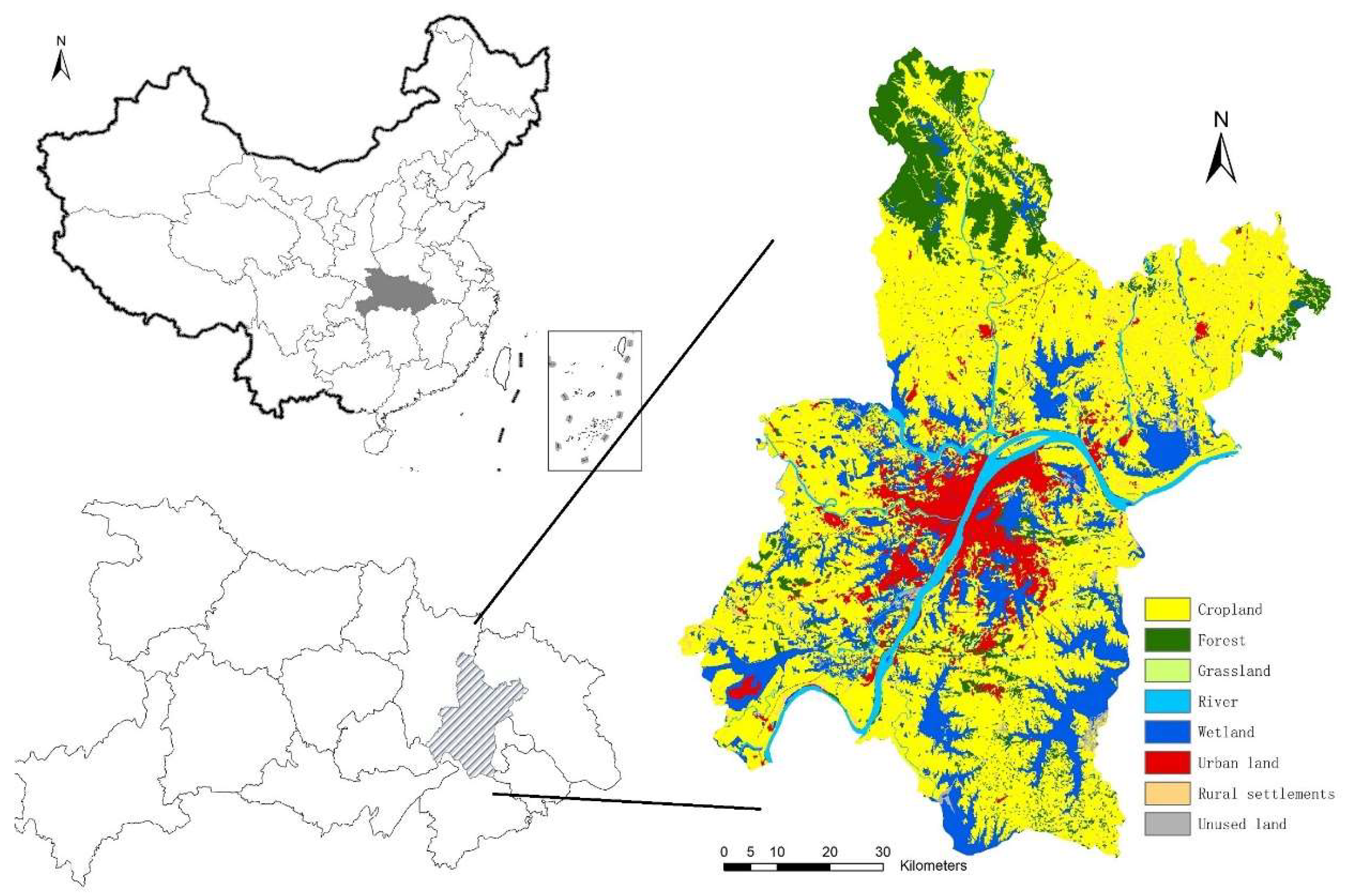
Wuhan, the provincial capital of Hubei province, is located in the middle of China. It covers an area of 8494 km² and resides by about 10.8 million population according to 2017 statistical bulletin for national economic and social development in Wuhan (Figure 2). The Yangtze River and Han River meet in the center of Wuhan, which makes it a distinct area with fertile soil. The cropland of Wuhan accounts for 55% of the total area. Wuhan also has a high proportion of ecological lands, and more than 160 lakes. Since 1978, Wuhan has experienced rapid urbanization which resulted excessive loss of lakes and ecological areas. Under these circumstances, most lakes in Wuhan have been shrunk [34], which leads to frequent urban waterlogging. As a result, land competition among urban expansion, cropland protection and ecosystem conservation turn out to be serious in Wuhan. Thus, we selected Wuhan as our study area to explore impacts of strict cropland protection on water yield.

2.2. Development of Future Land Use Scenarios

Since 1996, the Chinese government has implemented a series of strict cropland protection policies, such as Cropland Balance Policy, to mitigate cropland loss and guarantee food security [35,36]. These policies focus on the balance of cropland loss occupied by construction and cropland compensation, which requires that if cropland was occupied by constructive land, the developer must reclaim the same area of cropland in other places. Thus, to investigate the impacts of strict cropland protection on water yield, we developed two land use scenarios, differing in the implementation of strict cropland protection. One is a No Cropland Protection scenario (NCP), which assumes the land use change trend will be continued in the future without strict cropland protection policy. The other one is a Strict Cropland Protection scenario (SCP), which implements the strict cropland protection policy during urbanization. Each of them has the same quantities of urban land and rural settlements to ensure the comparability.

The only difference between the two scenarios is the demand of cropland (

Table 1. Cropland demands in different land use scenarios (ha).

	Observed in 2013	NCP	SCP
Cropland demand (ha)	460,716	-	460,716

NCP: No Cropland Protection scenario; SCP: Strict Cropland Protection scenario.

). In this research, cropland may be occupied by urban land and rural settlements under all scenarios. In the SCP scenario, ecological lands can be converted to cropland, while in the NCP scenario they cannot. In the SCP scenario, the demand of cropland is exactly the same as its quantity in 2013 because of cropland loss in quantity would not happen under the SCP scenario. While in the NCP scenario, there is no cropland demand for compensation.

2.3. Land Use Simulation in Different Scenarios

The cellular automata (CA) model has been proved as one of the most powerful tools to simulate land use changes due to its good performance and flexibility [37,38,39]. As one of the CA-based models, LANDSCAPE model has its own superiority apart from the advantages of CA-based models [40]. It can perform accurately changes of multiple land uses with a hierarchical allocation strategy, transition probability and transition intervals [40]. For this reason, we employed the LANDSCAPE model to simulate land use in 2030 for both scenarios.

In the hierarchical allocation strategy, the land use types are divided into active and passive ones by following White and Engelen [41]. Active land use change is driven by the demand of human and social development, such as urban land and cropland. Comparatively, change of passive land use types is resulted from the changes of the active ones (the losses of forest and wetland caused by urban expansion, for example).

The transition probability, which indicates the probability of a cell to be transformed to a target land use type, is determined by suitability and resistance. Suitability is the parameter that represents the attractiveness of a cell to be transformed to a land use type. Resistance is the transition difficulty for a cell to change its current state. The transition probability is determined by the following formula:

$$TT{P}_{i,t}=\frac{S_{i,t}}{R_{i,c}}$$

(1)

where $TT{P}_{i,c}$ is the total transition probability for cell $i$ to be transformed to land use type $t$; $S_{i,t}$ is the suitability of cell $i$ for the land use type $t$; $R_{i,c}$ represents the resistance of cell $i$ to be transformed from its current land use type to another. The higher value of $TT{P}_{i,t}$ means the higher probability of cell $i$ to be converted to the target land use type $t$.

The suitability $S_{i,t}$ is calculated by the equation as follows:

$$S_{i,t}=\left(1+{\left(-\ln \gamma \right)}^{\alpha }\right)\times P{G}_{i,t}\times Con\left(C_{i,t}\right)\times {\Omega }_{i,t}$$

(2)

where $\gamma$ is a random number changing from 0 to 1, and $\alpha$ is a dispersion number to control the stochastic number; $P{G}_{i,t}$ represents the impacts of environmental parameters in cell $i$, such as soil and accessible conditions, which is calculated by C5.0 decision tree algorithm in this research; $Con\left(C_{i,t}\right)$ is the constraint of the transition in cell $i$ with 1 for changeable and 0 for unchangeable; ${\Omega }_{i,t}$ is the neighborhood effect for target land use type $t$.

Resistance represents the difficulty of a cell to change to another land use type. The higher value of resistance means the higher transition difficulty. It can be calculated from the observed land use maps and we adopted the same resistances used by Zheng et al. because these have been proved suitable for simulating land use change in Wuhan [29].

As a CA-based model, LANDSCAPE model also needs transition intervals as the parameters. Transition interval represents the evolving rate for cells. We calculated the transition intervals by following Ke et al. [42].

The LANDSCAPE model should be calibrated before being applied to simulate land use changes [30]. Specifically, six steps are needed to calibrate the LANDSCAPE model: (1) define active and passive land use types and get the demands of active land use types in the observed land use map; (2) calculate the transition possibility for each land use type with C5.0 decision tree algorithm; (3) figure out the asynchronous transition intervals based on the changed cells in two observed land use maps at different time point; (4) calculate the resistances of land use types; (5) simulate land use change from 2000 to 2013 with the parameters mentioned above; and (6) assess the accuracy of the model by Kappa Simulation with the Map Comparison Kit, which was developed by the Netherlands Environmental Assessment Agency (PBL) [40,43].

2.4. Calculation of Water Yield in Different Land Use Scenarios

Water Yield module in the InVEST model was employed to calculate water yield in different land use scenarios. As one of the models for evaluation of ecosystem services, the performance of the InVEST model has been proved by many researches, including carbon storage, phosphorous reduction, water yield and biodiversity [44,45,46].

In the Water Yield module of the InVEST model, water yield can be calculated based on the Budyko curve and annual average precipitation [47]. According to the theory of water balance, water yield in each cell in the Water Yield module is calculated in accordance with the difference between precipitation and evapotranspiration, which can be represented by the following formula:

$$Y_{ij}=\left(1-\frac{E_{ij}}{P_{ij}}\right)\times P_{ij}$$

(3)

where $Y_{ij}$ is the water yield of land use type $i$ on cell $j$; $P_{ij}$ is the annual average rainfall of land use type $i$ on cell $j$; $E_{ij}$ is the actual evapotranspiration of land use type $i$ on cell $j$; $\frac{E_{ij}}{P_{ij}}$ is calculated by the Budyko curve proposed by Zhang et al. [48]:

$$\frac{E_{ij}}{P_{ij}}=1+\frac{P{E}_{ij}}{P_{ij}}-{\left[1+{(\frac{P{E}_{ij}}{P_{ij}})}^{{\alpha }_{i}j}\right]}^{1/{\alpha }_{ij}}$$

(4)

where $P{E}_{ij}$ is the potential evapotranspiration of land use type $i$ on cell $j$; ${\alpha }_{ij}$ is the non-physical factor that characterizes soil properties in natural climate. $P{E}_{ij}$ is defined by the Formula (5) as follows:

$$P{E}_{ij}=C_{ij}\times E{T}_{ij}$$

(5)

where $C_{ij}$ is the vegetation evapotranspiration coefficient of land use type $i$ on cell $j$, which is largely decided by the vegetative characteristics of the land use in the pixel; $E{T}_{ij}$ is the reference evapotranspiration of land use type $i$ on cell $j$.

${\alpha }_{ij}$ is defined by Formula (6):

$${\alpha }_{ij}=\mathrm{Z}\times \frac{A{W}_{ij}}{P_{ij}}+1.25$$

(6)

where $A{W}_{ij}$ is the volumetric plant-available water content, decided by the soil texture and effective rooting depth. $\mathrm{Z}$ is an empirical constant for seasonality factor.

2.5. Data Sources

2.5.1. Datasets for Land Use Simulation

Five categories of datasets are needed for land use simulation by using the LANDSCAPE model: land use datasets, accessibility datasets, soil datasets, terrain datasets, and meteorological datasets (

Table 2. Datasets for the LANDSCAPE model.

Datasets	Data Name	Meaning and Data Extraction Method
Land use datasets	Land use map in 2000	Land use map in 2000 based on land use database of resources and environment data center of Chinese Academy of Sciences (http://www.resdc.cn/)
	Land use map in 2013	Land use map in 2013 based on land use database of resources and environment data center of Chinese Academy of Sciences (http://www.resdc.cn/)
Accessibility datasets	Distance to highway	Euclidean distance to the nearest highway
	Distance to railway	Euclidean distance to the nearest railway
	Distance to state road	Euclidean distance to the nearest state road
	Distance to provincial road	Euclidean distance to the nearest provincial road
	Distance to county road	Euclidean distance to the nearest county road
	Distance to main road	Euclidean distance to the nearest main road
	Distance to other road	Euclidean distance to the nearest other road
Soil datasets	Soil_p	Soil phosphorus content
	Soil_ph	Soil PH
	Soil_organic_matter	Soil organic matter content
Terrain datasets	Digital elevation model (DEM)	Digital Elevation Model
	Slope	Slope extracted from DEM dataset
Meteorological datasets	Temperature	Annual average accumulated temperature
	Precipitation	Annul precipitation

). Observed land use maps in 2000 and 2013 needed for the LANDSCAPE model plays four roles in land use simulation: (1) to calculate the transition possibilities and asynchronous transition intervals; (2) to figure out the demands for active land uses; (3) to calibrate the LANDSCAPE model; and (4) to be as the initial land use map for simulation.

Land use datasets required for this research were obtained from the Data Centre of Resources and Environment, Chinese Academy of Science (http://www.resdc.cn/). Eight types of land use viz. cropland, forest, grassland, river, wetland, urban land, rural settlements, and unused land, were referred in the land use maps [49]. Because the maximum size of the input data allowed in the current LANDSCAPE model is 4000 $\times$ 4000 cells, the spatial resolution of land use maps was resampled from 30 m to 100 m through the ArcGIS10.2 “Resample” function.

Accessibility is proxied with the nearest distance to the target destination. Accessibility datasets for the study are: highway, railway, state roads, provincial roads, county roads, main roads and other roads in a city. All datasets of those roads were extracted from the Traffic Atlas of Wuhan with the following steps: (1) scan the traffic map into a digital map; (2) correct the digital map to the spatial reference of land use datasets; and (3) translate the digital map into shapefile. Then, we used “Euclidean Distance” tool in ArcGIS 10.2 to generate the raster datasets of the distance to the nearest road networks for each cell.

The soil datasets were collected to calculate the suitability map in land use simulation in this research, and mainly refer to three parameters: soil phosphorus content, soil PH, and soil organic matter content. All the soil datasets were obtained from the China Soil Database (http://gis.soil.csdb.cn/) in shapefile format. We converted the shapefile soil datasets into raster formats with a spatial resolution of 100 m, to keep consistence with the land use datasets.

Two categories of terrain datasets, digital elevation model (DEM) and slope, were used to calculate the suitability map in this research. The DEM dataset was acquired from the Shuttle Radar Topography Mission (SRTM), which is conducted by the National Aeronautics and Space Administration of USA (NASA) and USA National Geospatial-Intelligence Agency (NGA) [50]. The spatial resolution of the DEM dataset from SRTM in the study area is 90 m originally, but we resampled it to 100 m to consist with the resolution of land use datasets. Then, the slope raster was generated by the DEM data by using the “Slope” tool in ArcGIS10.2.

Two meteorological datasets were used to calculate the suitability map in the LANDSCAPE model: annual average accumulated temperature and annul precipitation. Both of the two meteorological datasets were obtained from the ground meteorological observatory in Hubei Province, China (http://data.cma.cn/). Then, Kriging tool in ArcGIS 10.2 was used to generate raster datasets of meteorological data from the observatory.

2.5.2. Datasets for Water Yield Calculation

Seven categories of datasets are needed for water yield calculation by using the Water Yield module in the InVEST model, including root restricting layer depth, land use maps, precipitation, evapotranspiration, plant available water content, watersheds, and biophysical table.

The root restricting layer depth data is from the Second National Soil Survey (http://gis.soil.csdb.cn/) and Kriging tool of ArcGIS10.2 was used to generate raster dataset of it with spatial resolution of 100 m. Land use maps comprise historical and simulated datasets used in Water Yield module in which historical land use maps from the Data Centre of Resources and Environment, Chinese Academy of Science and simulated land use maps were generated by the LANDSCAPE model. The precipitation data is from the ground meteorological observatory in Hubei Province (http://data.cma.cn/) and we employed the “Kriging” tool in ArcGIS10.2 to translate the data into raster data with a spatial resolution of 100 m. The evapotranspiration data was calculated by Formula (5) and then Kriging spatial interpolation method was used to generate a raster of evapotranspiration. The plant available water content is important for agricultural production and green plants growth, which can be calculated by soil texture and effective rooting depth with Formula (7):

$$A{W}_{ij}=Min\left(l{d}_{ij},r{d}_{ij}\right)\times PAWC$$

(7)

where $l{d}_{ij}$ is root restricting layer depth of land use type $i$ on cell $j$; $r{d}_{ij}$ is vegetation rooting depth of land use type $i$ on cell $j$; $PAWC$ is the plant available water capacity, which is the difference between field capacity and wilting point.

The watershed data is a shapefile data, which is generated with hydrological tools in ArcGIS10.2 with DEM data. The biophysical table contains parameters such as land use codes, name of each land use type, the equation used to calculate the actual evapotranspiration, the maximum vegetated root depth of land use types, and the evapotranspiration coefficient of each land use type. The land use codes and name of each land use type are defined by the authors while the others are obtained from the sample that given by the InVEST user guide (http://data.naturalcapitalproject.org/nightly-build/invest-users-guide/html/).

3. Results

3.1. Calibration of LAND System Cellular Automata for Potential Effects (LANDSCAPE) Model

To calibrate LANDSCAPE model, land use map in 2013 (Figure 3c) was simulated based on land use map in 2000 (Figure 3a). The Kappa Simulation index instead of Kappa coefficient was employed to assess the accuracy of the LANDSCAPE model by comparing the simulated land use map in 2013 and the observed one (Figure 3b) [51]. Kappa Simulation can distinguish the changed and unchanged cells, and only calculates the accuracy of the changed cells. Since most cells in the simulation period remain unchanged, the Kappa coefficient may result in an overestimation in accuracy while Kappa Simulation score can avoid the overestimation well. The value of Kappa Simulation score ranges from −1 to 1, where 1 represents a perfect match between the simulation result and the observed land use map, 0 indicates a random distribution of the simulation results and −1 shows no agreement between the simulation result and the observed target land use map.

Table 3. Kappa Simulation scores of each land use type in the simulated result.

Land Use Type	Cropland	Forest	Grassland	Wetland	Urban Land	Rural Settlements	Unused Land
Kappa Simulation	0.227	0.109	0.074	0.115	0.438	0.058	0.181
KTransLoc	0.430	0.302	0.153	0.462	0.469	0.183	0.364
KTransition	0.529	0.359	0.484	0.248	0.934	0.316	0.499

shows the Kappa Simulation score of each land use type. As we can see, the Kappa simulation scores of each land use type are all greater than 0, which means that LANDSCAPE model is accurate enough to simulate land use change in Wuhan. Specifically, the Kappa Simulation scores of urban land and cropland are 0.438 and 0.227 respectively, indicating that the simulation results of these land uses types are higher and reliable. The Kappa Simulation score of rural settlements is close to 0. That is because rural settlements in China are highly dispersed [52], which is really hard to simulate. But the KTransition score of rural settlements is 0.316, indicating the high accuracy of land use type transition [51].

3.2. Land Use Change in Different Scenarios

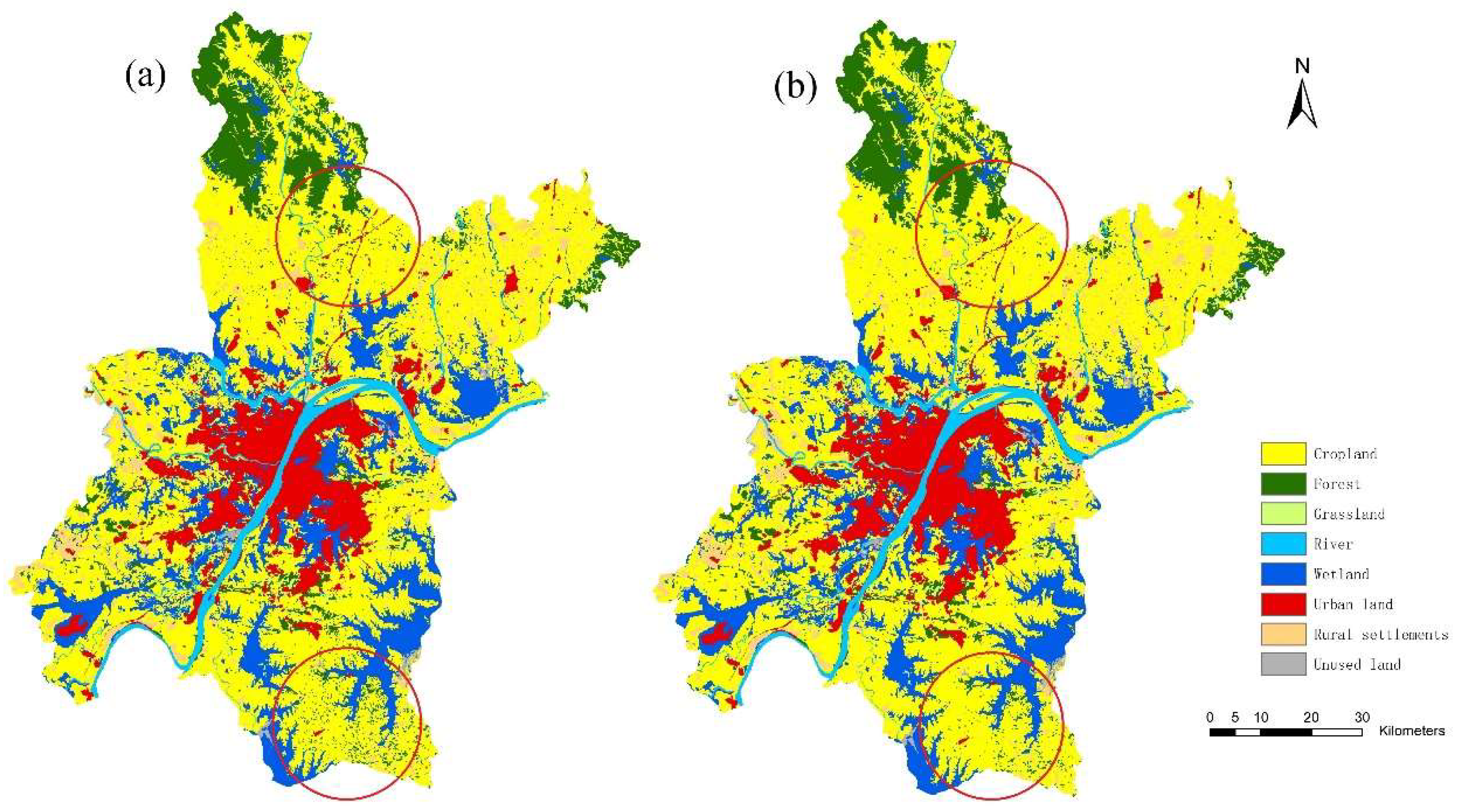
Figure 4 illustrates simulated land use maps of Wuhan in 2030 in two different scenarios: NCP (a) and SCP (b). The changes of urban land and rural settlements are similar in both NCP and SCP scenarios during 2013 and 2030, while the changes of other land use types, such as forest, wetland, and grassland, show more differences.

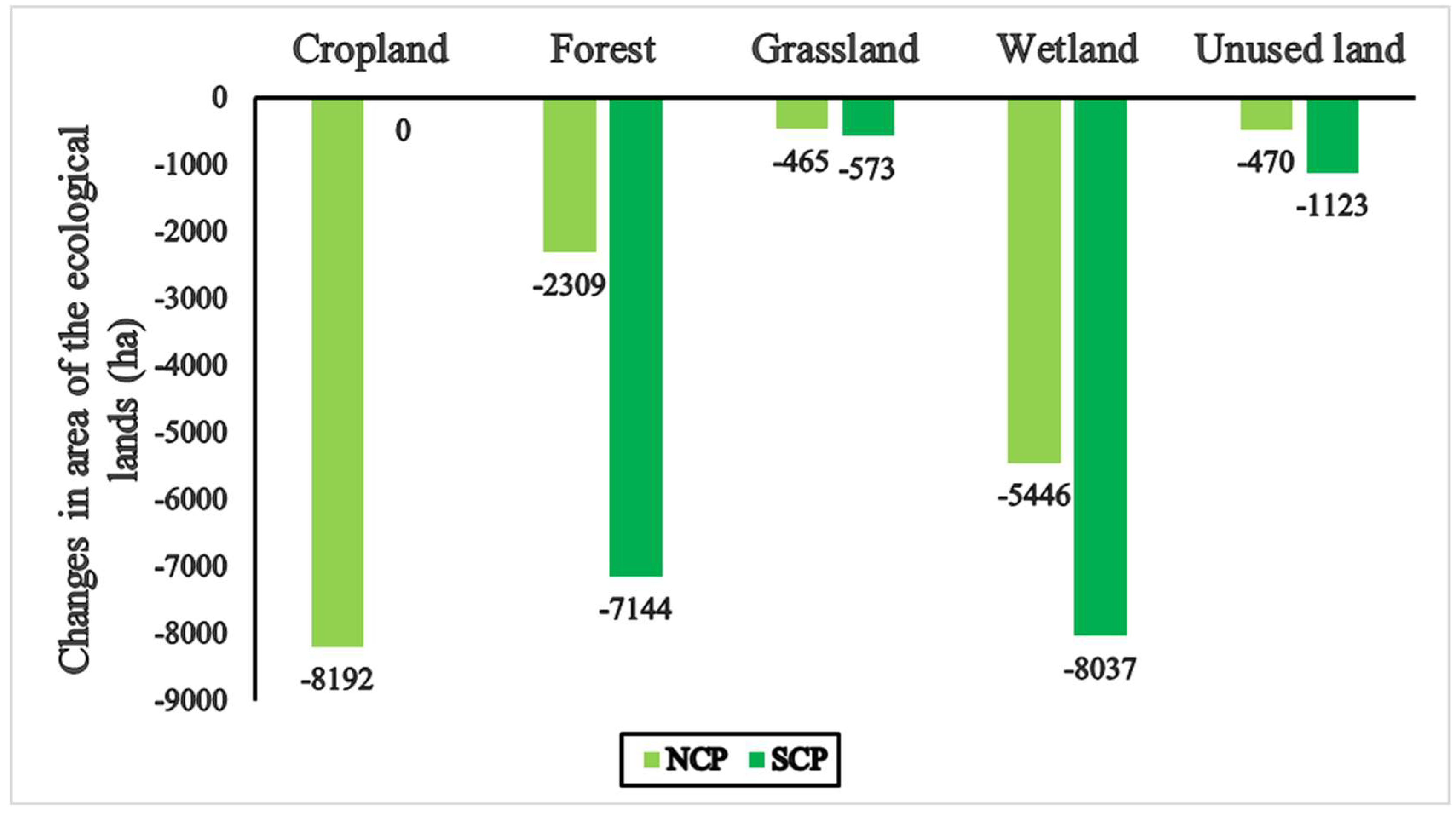
Figure 5 shows loss of individual land use types in different scenarios in Wuhan in 2030. The land use change pattern is quite different in the two scenarios, making the different loss of cropland and other lands. There is no loss of cropland in quantity in the SCP scenario that is because we gave a certain demand of cropland in the LANDSCAPE model, while 8192 ha of cropland would be taken up by built-up area expansion in the NCP scenario. To other land use types, loss of forest is 2309 ha in NCP scenario and 7144 ha in SCP scenario separately. The loss of wetland is 5446 ha in the NCP scenario and 8037 ha in the SCP scenario. Strict cropland protection makes more forest (4835 ha) and wetland (2591 ha) convert to cropland in the SCP scenario.

3.3. Water Yield in Different Scenarios

Table 4. Water yield in the two scenarios in Wuhan (10⁷ m³).

Scenario	Total Water Yield	The Changes of Water Yield
NCP	659.36	8.72
SCP	660.08	9.44

NCP: No Cropland Protection scenario; SCP: Strict Cropland Protection scenario.

demonstrates the total water yield in 2030 and the changes of water yield during 2013–2030 in scenarios of NCP and SCP. The total water yields in 2030 in the NCP and SCP scenarios are ${659.36\times 10}^7$ m³ and ${660.08\times 10}^7$ m³, respectively. Compared with quantity of water yield in 2013 (${650.64\times 10}^7$ m³), water yield in 2030 in both scenarios would increase. However, the quantity of water yield increase in two different scenarios would be different. Specifically, water yield would increase ${8.72\times 10}^7$ m³ in the NCP scenario during 2013–2030, while it would increase ${9.44\times 10}^7$ m³ in the SCP scenario. The difference is ${0.72\times 10}^7$ m³.

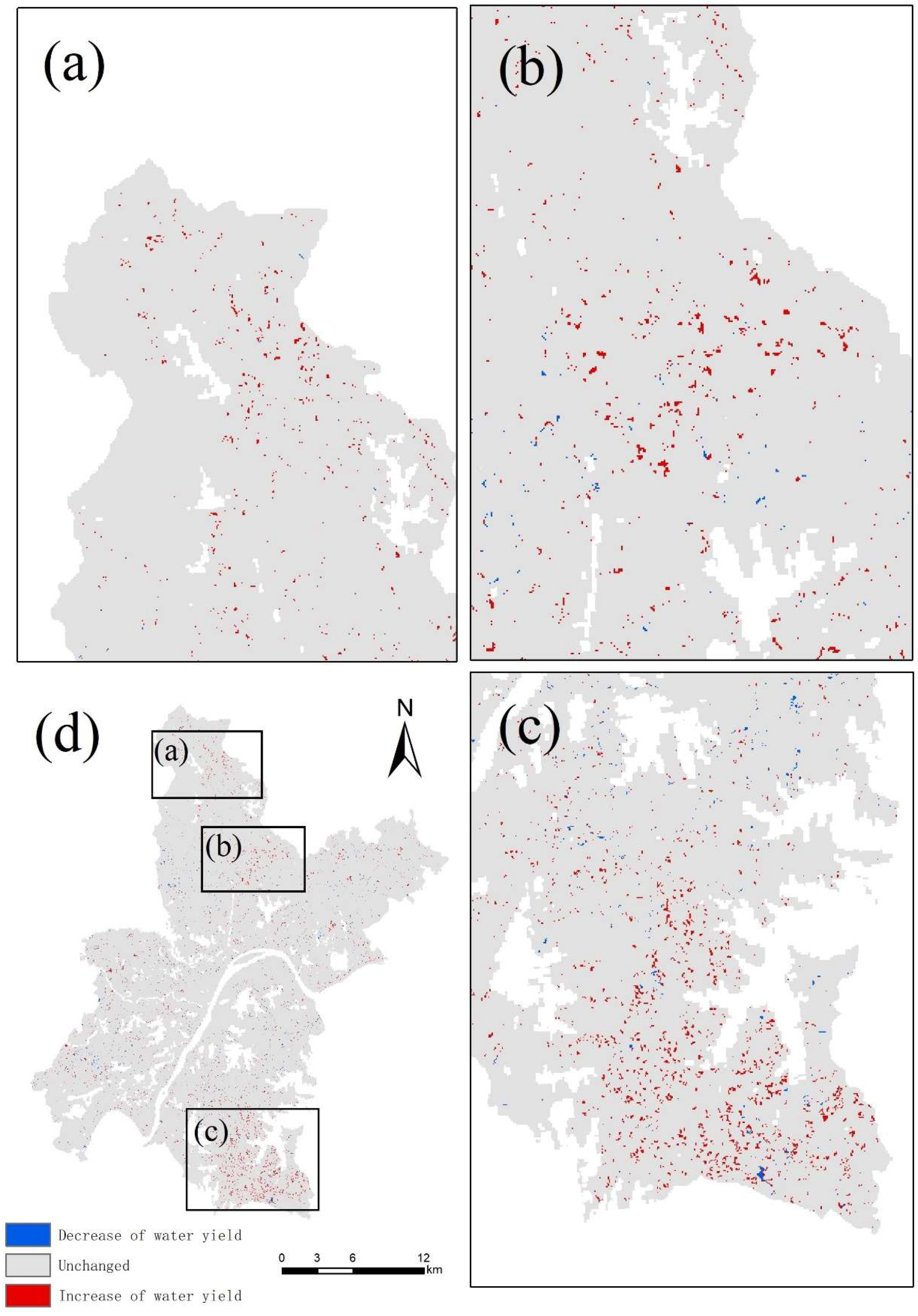
Figure 6 shows the spatial differences of water yield between the NCP and SCP scenarios. Increase in water yield from the NCP scenario to the SCP scenario would happen dominantly in regions with a total of 9301 ha while decrease would appear in regions with a total of 2700 ha. Specifically, regions with increase of water yield are distributed around the city separately, but mainly located in the southeast (Figure 6c), north (Figure 6b) and northwest (Figure 6a) of Wuhan where these are the main areas of forest loss.

The land use change patterns of regions with increase and decrease of water yield in the scenarios of NCP and SCP are quite different (

Table 5. The quantities of each land use type in regions with decrease and increase of water yield from No Cropland Protection scenario to Strict Cropland Protection scenario (ha).

Region	Decrease of Water Yield		Increase of Water Yield
Scenario	NCP	SCP	NCP	SCP
Cropland	14	2400	1731	7331
Forest	0	69	4939	30
Grassland	23	60	14	0
Wetland	132	86	2527	0
Urban land	818	53	14	803
Rural settlements	1098	32	58	1137
Unused land	615	0	18	0
Total	2700	2700	9301	9301

NCP: No Cropland Protection scenario; SCP: Strict Cropland Protection scenario.

). In regions with a decrease of water yield, land use is mainly composed of urban land, rural settlements and unused land in NCP scenario, which contribute 30.3%, 40.7% and 22.8% respectively; while cropland seizes the largest part of 88.9% in the SCP scenario. As for regions with an increase of water yield, land use mainly consisted of ecological lands in the NCP scenario, such as forest (4939 ha, 47.2%) and wetland (2527 ha, 27.2%); while cropland and rural settlements contribute 78.8% and 12.2% in the SCP scenario.

4. Discussion

Rapid urbanization which causes significant land use change has been considered as an important factor for changes of water yield and ecosystem services [21,22,38,53]. However, as an incident effect of urban expansion, impact of land use changes initiated by cropland protection usually has been overlooked by most studies. Trying to explore this issue, we simulated future land use changes under two different scenarios, with strict or without cropland protection (SCP and NCP) at the same level of urbanization with by using the LANDSCAPE model and calculated the water yield with the Water Yield module in the InVEST model. To guarantee the relative accuracy of the land use change model in this research, we used the observed land use maps of the study region in 2000 and 2013 to calibrate the model [40]. The calibration results showed that the simulated land use map in 2013 has relative high Kappa Simulation scores, which means the model is trustworthy [51]. We also compared our water yield results with similar research in karst mountain areas of China [54] and in South Korea [55]. The average water yield in the observed land use map 2013 in our study is 759 mm, lower than that in karst mountain areas of China and South Korea. That is because the former has a relative lower latitude and the latter is surrounded by sea, which makes their precipitation higher than our study area.

The simulation results show that build-up area expansion definitely leads to vast loss of cropland and ecological land, and to maintain the strict cropland protection, the ecological land will lose more, which is similar to the results of Zheng et al. [29]. Furthermore, we calculated the water yield in different scenarios showing that urbanization will increase the water yield and the strict cropland protection will aggravate this phenomenon. The results show that the total water yield would increase ${8.72\times 10}^7$ m³ in the NCP scenario and ${9.44\times 10}^7$ m³ in the SCP scenario. The difference between the two scenarios is ${0.72\times 10}^7$ m³, which is almost equal to the water capacity of a small reservoir according to the Classification and Design Standard of Water Conservancy and Hydropower Project in China. That is because built-up area takes up lots of cropland and ecological lands, resulting in an increase of the impervious surface. The impervious surface leads the increase of surface runoff and the reduce of evapotranspiration [24,25]. So, if the precipitation remains unchanged, the total water yield will increase. To ensure food security, the Chinese government has put forward the strictest cropland protection policy in the world, which keeps the cropland balance in quantity [35]. Studies have demonstrated that the water retention capacity of ecological land such as forest and wetland is more powerful than cropland [56] and the decreasing sequence of water yield of different land use types mainly conform with urban land, rural settlements, unused land, grassland, cropland, forest and wetland [57]. In the SCP scenario, due to the strict cropland protection, wetland and forest are converted to cropland, leading the indirect losses of ecological lands (Figure 5). Therefore, the water retention capacity is becoming relatively lower compared to that with no cropland protection due to the indirect loss of ecological land caused by strict cropland protection. That is the reason why the water yield in the SCP scenario is higher than that in NCP scenario.

As one of the most important ecosystem services, water yield plays a vital role for sustainable development. Previous studies have demonstrated that water supply is a basic condition for human life [9,10,11] and it is important at the basin scale [58,59]. Is the increased water yield really a good thing for a rapid urbanizing city like Wuhan? Maybe it is not. There is no doubt that the impervious surface will increase in the future since urbanization is still the trend of future development and it will definitely take up lots of cropland, forest and wetland. Meanwhile, the rivers, lakes and urban drainage system are facing the pressure of increased surface runoff. It has been proved that forest and wetland are the most important land use types that can conserve water and reduce the probability of floods [60]. However, the indirect losses of forest and wetland caused by strict cropland protection leads the water yield and surface runoff to increase. It will also bring environmental problems, such as soil erosion. Thus, if a rapid urbanization city implements the strict cropland protection policy, the possibility of floods occurring is higher.

Also, there are some limitations of our study. Firstly, we developed the land use scenarios only based on the cropland protection policies that implemented in China. As we all know, policies will change among countries. So, the methodology can be applied in different research areas but the parameters in the scenarios should be changed to meet local policies. Secondly, to ensure the comparability we did not consider the effect of climate change, although studies have shown it influences the water yield [17,26]. Thus, future studies could combine climate change models with the models we use.

5. Conclusions

This study focuses on the impacts of strict cropland protection on water yield by combining the LANDSCAPE model and the Water Yield module in the InVEST model in two different land use scenarios (NCP and SCP). The results show that implementation of strict cropland protection would lead to an increase of water yield from 2013 to 2030 (${0.72\times 10}^7$ m³), compared to that without strict cropland protection. Considering the double pressure of urbanization and cropland compensation on water yield, it is not wise to implement strict cropland protection in an area undergoing rapid urbanization.

References

1. Watson, R.T.; Rosswall, T.; Steiner, A.; Töpfer, K.; Arico, S.; Bridgewater, P. Ecosystems and Human Well-Being; Island Press: Washington, DC, USA, 2005; ISBN 1559634022. [Google Scholar]
2. Costanza, R.; de Groot, R.; Sutton, P.; van der Ploeg, S.; Anderson, S.J.; Kubiszewski, I.; Farber, S.; Turner, R.K. Changes in the global value of ecosystem services. Glob. Environ. Chang. 2014, 26, 152–158. [Google Scholar] [CrossRef]
3. Su, S.; Xiao, R.; Jiang, Z.; Zhang, Y. Characterizing landscape pattern and ecosystem service value changes for urbanization impacts at an eco-regional scale. Appl. Geogr. 2012, 34, 295–305. [Google Scholar] [CrossRef]
4. Tesfaye, A.; Brouwer, R.; van der Zaag, P.; Negatu, W. Assessing the costs and benefits of improved land management practices in three watershed areas in Ethiopia. Int. Soil Water Conserv. Res. 2016, 4, 20–29. [Google Scholar] [CrossRef] [Green Version]
5. Costanza, R.; de Groot, R.; Braat, L.; Kubiszewski, I.; Fioramonti, L.; Sutton, P.; Farber, S.; Grasso, M. Twenty years of ecosystem services: How far have we come and how far do we still need to go? Ecosyst. Serv. 2017, 28, 1–16. [Google Scholar] [CrossRef]
6. Olander, L.P.; Johnston, R.J.; Tallis, H.; Kagan, J.; Maguire, L.A.; Polasky, S.; Urban, D.; Boyd, J.; Wainger, L.; Palmer, M. Benefit relevant indicators: Ecosystem services measures that link ecological and social outcomes. Ecol. Indic. 2018, 85, 1262–1272. [Google Scholar] [CrossRef]
7. Xie, G.; Zhang, C.; Zhen, L.; Zhang, L. Dynamic changes in the value of China’s ecosystem services. Ecosyst. Serv. 2017, 26, 146–154. [Google Scholar] [CrossRef]
8. United Nations General Assembly. Transforming Our World: The 2030 Agenda for Sustainable Development; UN: New York, NY, USA, 2015. [Google Scholar]
9. Wang, C.; Blackmore, J.M. Resilience Concepts for Water Resource Systems. J. Water Resour. Plan. Manag. 2009. [Google Scholar] [CrossRef]
10. Kang, S.; Hao, X.; Du, T.; Tong, L.; Su, X.; Lu, H.; Li, X.; Huo, Z.; Li, S.; Ding, R. Improving agricultural water productivity to ensure food security in China under changing environment: From research to practice. Agric. Water Manag. 2017, 179, 5–17. [Google Scholar] [CrossRef]
11. Zhang, Y.; Chen, M.; Zhou, W.; Zhuang, C.; Ouyang, Z. Evaluating Beijing’s human carrying capacity from the perspective of water resource constraints. J. Environ. Sci. 2010, 22, 1297–1304. [Google Scholar] [CrossRef]
12. Weindl, I.; Bodirsky, B.L.; Rolinski, S.; Biewald, A.; Lotze-Campen, H.; Müller, C.; Dietrich, J.P.; Humpenöder, F.; Stevanović, M.; Schaphoff, S.; et al. Livestock production and the water challenge of future food supply: Implications of agricultural management and dietary choices. Glob. Environ. Chang. 2017, 47, 121–132. [Google Scholar] [CrossRef]
13. Rockstrom, J.; Lannerstad, M.; Falkenmark, M. Assessing the water challenge of a new green revolution in developing countries. Proc. Natl. Acad. Sci. USA 2007, 104, 6253–6260. [Google Scholar] [CrossRef] [PubMed] [Green Version]
14. Kosolapova, N.A.; Matveeva, L.G.; Nikitaeva, A.Y.; Molapisi, L. Modeling resource basis for social and economic development strategies: Water resource case. J. Hydrol. 2017, 553, 438–446. [Google Scholar] [CrossRef]
15. Setlhogile, T.; Arntzen, J.; Pule, O.B. Economic accounting of water: The Botswana experience. Phys. Chem. Earth 2017, 100, 287–295. [Google Scholar] [CrossRef]
16. Laino-Guanes, R.; González-Espinosa, M.; Ramírez-Marcial, N.; Bello-Mendoza, R.; Jiménez, F.; Casanoves, F.; Musálem-Castillejos, K. Human pressure on water quality and water yield in the upper Grijalva river basin in the Mexico-Guatemala border. Ecohydrol. Hydrobiol. 2016, 16, 149–159. [Google Scholar] [CrossRef]
17. Salerno, F.; Viviano, G.; Tartari, G. Urbanization and climate change impacts on surface water quality: Enhancing the resilience by reducing impervious surfaces. Water Res. 2018, 144, 491–502. [Google Scholar] [CrossRef] [PubMed]
18. Kim, N.W.; Won, Y.S.; Lee, J.; Lee, J.E.; Jeong, J. Hydrological Impacts of Urban Imperviousness in White Rock Creek Watershed. Trans. ASABE 2011, 54, 1759–1771. [Google Scholar] [CrossRef]
19. Cuo, L.; Beyene, T.K.; Voisin, N.; Su, F.; Lettenmaier, D.P.; Alberti, M.; Richey, J.E. Effects of mid-twenty-first century climate and land cover change on the hydrology of the Puget Sound basin, Washington. Hydrol. Process. 2011, 25, 1729–1753. [Google Scholar] [CrossRef]
20. Wang, C.; Hou, Y.; Xue, Y. Water resources carrying capacity of wetlands in Beijing: Analysis of policy optimization for urban wetland water resources management. J. Clean. Prod. 2017, 161, 1180–1191. [Google Scholar] [CrossRef]
21. Nie, W.; Yuan, Y.; Kepner, W.; Nash, M.S.; Jackson, M.; Erickson, C. Assessing impacts of Landuse and Landcover changes on hydrology for the upper San Pedro watershed. J. Hydrol. 2011, 407, 105–114. [Google Scholar] [CrossRef]
22. Ayivi, F.; Jha, M.K. Estimation of water balance and water yield in the Reedy Fork-Buffalo Creek Watershed in North Carolina using SWAT. Int. Soil Water Conserv. Res. 2018, 6, 203–213. [Google Scholar] [CrossRef]
23. Lin, T.; Liu, X.; Song, J.; Zhang, G.; Jia, Y.; Tu, Z.; Zheng, Z.; Liu, C. Urban waterlogging risk assessment based on internet open data: A case study in China. Habitat Int. 2018, 71, 88–96. [Google Scholar] [CrossRef]
24. Arnold, C.L.; Gibbons, C.J. Impervious Surface Coverage: The Emergence of a Key Environmental Indicator. J. Am. Plan. Assoc. 1996, 62, 243–258. [Google Scholar] [CrossRef]
25. Redfern, T.W.; Macdonald, N.; Kjeldsen, T.R.; Miller, J.D.; Reynard, N. Current understanding of hydrological processes on common urban surfaces. Prog. Phys. Geogr. 2016, 40. [Google Scholar] [CrossRef]
26. Sunde, M.G.; He, H.S.; Hubbart, J.A.; Urban, M.A. An integrated modeling approach for estimating hydrologic responses to future urbanization and climate changes in a mixed-use midwestern watershed. J. Environ. Manage. 2018, 220, 149–162. [Google Scholar] [CrossRef] [PubMed]
27. US Army Corps of Engineers. Hydrologic Modeling System User’s Manual; US Army Corps of Engineers: Washington, DC, USA, 2008; ISBN CPD-74A.
28. Scordo, F.; Lavender, T.M.; Seitz, C.; Perillo, V.L.; Rusak, J.A.; Cintia Piccolo, M.; Perillo, G.M.E. Modeling Water Yield: Assessing the Role of Site and Region-Specific Attributes in Determining Model Performance of the InVEST Seasonal Water Yield Model. Water 2018, 10, 1496. [Google Scholar] [CrossRef]
29. Zheng, W.; Ke, X.; Zhou, T.; Yang, B. Trade-offs between cropland quality and ecosystem services of marginal compensated cropland—A case study in Wuhan, China. Ecol. Indic. 2018. [Google Scholar] [CrossRef]
30. Ke, X.; van Vliet, J.; Zhou, T.; Verburg, P.H.; Zheng, W.; Liu, X. Direct and indirect loss of natural habitat due to built-up area expansion: A model-based analysis for the city of Wuhan, China. Land Use Policy 2018, 74, 231–239. [Google Scholar] [CrossRef]
31. Zhong, T.; Huang, X.; Zhang, X.; Scott, S.; Wang, K. The effects of basic arable land protection planning in Fuyang County, Zhejiang Province, China. Appl. Geogr. 2012, 35, 422–438. [Google Scholar] [CrossRef]
32. Liu, X.; Zhao, C.; Song, W. Review of the evolution of cultivated land protection policies in the period following China’s reform and liberalization. Land Use Policy 2017, 67, 660–669. [Google Scholar] [CrossRef]
33. Song, W.; Pijanowski, B.C. The effects of China’s cultivated land balance program on potential land productivity at a national scale. Appl. Geogr. 2013, 46, 158–170. [Google Scholar] [CrossRef]
34. Yang, B.; Ke, X. Analysis on urban lake change during rapid urbanization using a synergistic approach: A case study of Wuhan, China. Phys. Chem. Earth 2015, 89–90, 127–135. [Google Scholar] [CrossRef]
35. Lichtenberg, E.; Ding, C. Assessing farmland protection policy in China. Land Use Policy 2008, 25, 59–68. [Google Scholar] [CrossRef]
36. Zhong, T.Y.; Huang, X.J.; Zhang, X.Y.; Wang, K. Temporal and spatial variability of agricultural land loss in relation to policy and accessibility in a low hilly region of southeast China. Land Use Policy 2011, 28, 762–769. [Google Scholar] [CrossRef]
37. Van Asselen, S.; Verburg, P.H. Land cover change or land-use intensification: Simulating land system change with a global-scale land change model. Glob. Chang. Biol. 2013, 19, 3648–3667. [Google Scholar] [CrossRef] [PubMed]
38. Verburg, P.H.; Tabeau, A.; Hatna, E. Assessing spatial uncertainties of land allocation using a scenario approach and sensitivity analysis: A study for land use in Europe. J. Environ. Manag. 2013, 127, S132–S144. [Google Scholar] [CrossRef]
39. García, A.M.; Santé, I.; Boullón, M.; Crecente, R. Calibration of an urban cellular automaton model by using statistical techniques and a genetic algorithm. Application to a small urban settlement of NW Spain. Int. J. Geogr. Inf. Sci. 2013, 27, 1593–1611. [Google Scholar] [CrossRef]
40. Ke, X.; Zheng, W.; Zhou, T.; Liu, X. A CA-based land system change model: LANDSCAPE. Int. J. Geogr. Inf. Sci. 2017, 31, 1798–1817. [Google Scholar] [CrossRef]
41. White, R.; Engelen, G. Cellular automata as the basis of integrated dynamic regional modelling. Environ. Plan. B Plan. Des. 1997. [Google Scholar] [CrossRef]
42. Ke, X.; Qi, L.; Zeng, C. A partitioned and asynchronous cellular automata model for urban growth simulation. Int. J. Geogr. Inf. Sci. 2016, 30, 637–659. [Google Scholar] [CrossRef]
43. Visser, H.; De Nijs, T. The map comparison kit. Environ. Model. Softw. 2006, 21, 346–358. [Google Scholar] [CrossRef]
44. Kovacs, K.; Polasky, S.; Nelson, E.; Keeler, B.L.; Pennington, D.; Plantinga, A.J.; Taff, S.J. Evaluating the Return in Ecosystem Services from Investment in Public Land Acquisitions. PLoS ONE 2013, 8, e062202. [Google Scholar] [CrossRef] [PubMed]
45. Nelson, E.; Mendoza, G.; Regetz, J.; Polasky, S.; Tallis, H.; Cameron, D.R.; Chan, K.M.A.; Daily, G.C.; Goldstein, J.; Kareiva, P.M.; et al. Modeling multiple ecosystem services, biodiversity conservation, commodity production, and tradeoffs at landscape scales. Front. Ecol. Environ. 2009, 7, 4–11. [Google Scholar] [CrossRef] [Green Version]
46. Yu, J.; Yuan, Y.; Nie, Y.; Ma, E.; Li, H.; Geng, X. The Temporal and Spatial Evolution of Water Yield in Dali County. Sustainability 2015, 7, 6069–6085. [Google Scholar] [CrossRef] [Green Version]
47. Sharp, R.; Tallis, H.T.; Ricketts, T.; Guerry, A.D.; Wood, S.A.; Chaplin-Kramer, R.; Nelson, E.; Ennaanay, D.; Wolny, S.; Olwero, N.; et al. InVEST User Guide: The Natural Capital Project; Stanford University: Stanford, CA, USA, 2016; ISBN 9780874216561. [Google Scholar]
48. Zhang, L.; Hickel, K.; Dawes, W.R.; Chiew, F.H.S.; Western, A.W.; Briggs, P.R. A rational function approach for estimating mean annual evapotranspiration. Water Resour. Res. 2004. [Google Scholar] [CrossRef]
49. Liu, J.; Zhang, Z.; Xu, X.; Kuang, W.; Zhou, W.; Zhang, S.; Li, R.; Yan, C.; Yu, D.; Wu, S.; et al. Spatial patterns and driving forces of land use change in China during the early 21st century. J. Geogr. Sci. 2010, 20, 483–494. [Google Scholar] [CrossRef]
50. Berry, P.A.M.; Garlick, J.D.; Smith, R.G. Near-global validation of the SRTM DEM using satellite radar altimetry. Remote Sens. Environ. 2007, 106, 17–27. [Google Scholar] [CrossRef]
51. Van Vliet, J.; Bregt, A.K.; Hagen-Zanker, A. Revisiting Kappa to account for change in the accuracy assessment of land-use change models. Ecol. Modell. 2011, 222, 1367–1375. [Google Scholar] [CrossRef]
52. Yang, R.; Liu, Y.; Long, H.; Qiao, L. Spatio-temporal characteristics of rural settlements and land use in the Bohai Rim of China. J. Geogr. Sci. 2015, 25, 559–572. [Google Scholar] [CrossRef] [Green Version]
53. He, C.; Liu, Z.; Tian, J.; Ma, Q. Urban expansion dynamics and natural habitat loss in China: A multiscale landscape perspective. Glob. Chang. Biol. 2014, 20, 2017. [Google Scholar] [CrossRef]
54. Lang, Y.; Song, W.; Deng, X. Projected land use changes impacts on water yields in the karst mountain areas of China. Phys. Chem. Earth 2018, 104, 66–75. [Google Scholar] [CrossRef]
55. Kim, G.S.; Lim, C.H.; Kim, S.J.; Lee, J.; Son, Y.; Lee, W.K. Effect of national-scale afforestation on forest water supply and soil loss in South Korea, 1971–20. Sustainabilty 2017, 9, 1017. [Google Scholar] [CrossRef]
56. Namugize, J.N.; Jewitt, G.; Graham, M. Effects of land use and land cover changes on water quality in the uMngeni river catchment, South Africa. Phys. Chem. Earth 2018, 105, 247–264. [Google Scholar] [CrossRef]
57. Lang, Y.; Song, W.; Zhang, Y. Responses of the water-yield ecosystem service to climate and land use change in Sancha River Basin, China. Phys. Chem. Earth 2017, 101, 102–111. [Google Scholar] [CrossRef]
58. Canqiang, Z.; Wenhua, L.; Biao, Z.; Moucheng, L. Water Yield of Xitiaoxi River Basin Based on InVEST Modeling. J. Resour. Ecol. 2012, 3, 50–54. [Google Scholar] [CrossRef]
59. Hoyer, R.; Chang, H. Assessment of freshwater ecosystem services in the tualatin and Yamhill basins under climate change and urbanization. Appl. Geogr. 2014, 53, 402–416. [Google Scholar] [CrossRef]
60. Alongi, D.M. Mangrove forests: Resilience, protection from tsunamis, and responses to global climate change. Estuar. Coast. Shelf Sci. 2008, 76, 1–13. [Google Scholar] [CrossRef]
Figure 1. Research framework.
Sustainability 11 00184 g001
Figure 2. Location and land use map of Wuhan.
Sustainability 11 00184 g002
Figure 3. Observed maps and simulated map for calibration: (a) observed land use map in 2000; (b) observed land use map in 2013; and (c) simulated land use map in 2013.
Sustainability 11 00184 g003
Figure 4. Simulated land use maps of Wuhan in 2030 in scenarios of: (a) No Cropland Protection scenario (NCP); and (b) Strict Cropland Protection scenario (SCP). The red circle demonstrates that more forest is converted to cropland in scenario with strict cropland protection (SCP scenario) compared to that without strict cropland protection (NCP scenario).
Sustainability 11 00184 g004
Figure 5. The loss of ecological lands in two different scenarios in Wuhan between 2013 and 2030.
Sustainability 11 00184 g005
Figure 6. Spatial differences of water yield between No Cropland Protection scenario (NCP) and Strict Cropland Protection scenario (SCP): (a) in the northwest, (b) north, (c) southeast, and (d) the whole area. Decrease of water yield indicates water yield in the SCP scenario is lower than that in the NCP scenario; Unchanged represents that water yield in the SCP scenario is equal to that in the NCP scenario; Increase of water yield demonstrates that water yield in SCP scenario is higher than that in the NCP scenario.
Sustainability 11 00184 g006