Adaptive Analysis of Green Space Network Planning for the Cooling Effect of Residential Blocks in Summer: A Case Study in Shanghai

Abstract

The effect of Urban Heat Islands (UHIs) is becoming increasingly serious in cities. Research on the adaptive planning policies for microthermal environments at the residential block level of cities is thus becoming of greater significance. Based on the cooling effect of planning control elements in residential block areas, the element effects characteristics of water bodies and vegetation distribution on the thermal environment of residential blocks were analyzed by using ENVI-met software. The simulation data analysis showed that the combination of water bodies and vegetation had a synergistic cooling effect. Based on these results, simulations of five effective adaptive measures were carried out step by step in planning scenarios, that is, improving the water bodies with vegetation corridors, the application of high-albedo material on streets, and increasing the number of green patches, east-west green corridors, and north-south green corridors. The results were as follows. First, although each of the five optimization strategies have a certain degree of cooling effect on the entire block, the superposition of each factor had a synergistic effect. Second, different spatial optimization strategies had different cooling ranges for each subzone. The optimization of the north-south green corridor, green patches, and water features corridors were particularly significant for microclimate cooling. The east-west green corridor has a certain influence on a certain range of downwind zones and had an auxiliary cooling effect. The high-albedo material also had a weak overall decrease function for the thermal environment. Finally, the downwind area of the urban creek network had a great impact on cooling intensity, with distance attenuation characteristics; it was also proposed that the comprehensive cooling effect of the green space network with optimized layout was greater than that of any single green space element. The optimization scenario planning research provided a method for improving the scientific distribution of adaptation measures in urban residential blocks.

1. Introduction

The Climate Change 2014 Synthesis Report stated that global surface temperature change for the end of the 21st century (2081–2100), compared with the years from 1850 to 1900, was projected to likely exceed 1.5 °C [1]. In the context of global warming, the impact of the urban heat island phenomenon will be exacerbated [2], the frequency of heat waves will be higher, and the risk of climate change will be more serious [3]. Facing the challenge of urban climate change, adaptive planning at the micro level has gradually become a hot topic in the academic field, compared with macrolevel cooling strategies [4]. The methods of planning for adaptive thermal environments of urban building blocks are becoming the main research area for the site-level of cities.

The analysis of the cause of urban heat islands shows that land use change is an important factor [5]. Many scholars have analyzed the biogeochemical effects of land use on climate [6], and land use changes have resulted in changes in the structure and properties of underlying surfaces [7]. Urbanization is the key factor of land use change [8]. Under the promotion of urbanization, a large number of land use types, such as vegetation and water bodies, are transformed into construction land [9]. Research on the Urban Heat Island (UHI) effect under the influence of urbanization had has been paid more and more attention in recent years [10]. China has experienced a rapid urbanization process [11], especially in the Yangtze River Delta, which has become one of the three urban agglomerations in China [12]. Rapid urbanization has brought economic development to China, but has also greatly changed the urban thermal environment to aggravate the urban heat island effect [13]. Based on the data of 41 meteorological stations in the Yangtze River Delta urban agglomeration, it was found that the average warming rates of the air temperature of huge cities, megalopolises, large cities, medium-sized cities, and small cities were 0.483, 0.314 ± 0.030, 0.282 ± 0.042, 0.225 ± 0.044, and 0.179 ± 0.046 °C/decade during the period of 1957–2013, respectively. In mega-cities such as Shanghai, the warming rate of average, minimal, and maximal air temperature were growing at an annual rate of 0.483 °C/decade, 0.521 °C/decade, and 0.433 °C/decade in the past 50 years, respectively [14]. With the passage of time, the difference of the four seasons of the heat island effect tends to be homogenized in Shanghai [15].

Recent research finds that temperature and relative humidity are important factors in assessing local climate change [16]. The water body can increase air humidity effectively through evapotranspiration, and the evapotranspiration effect will be better if there is a large area of greening [17]. The energy balance of a river is typically dominated by the net shortwave balance, followed by the net longwave balance and evaporative flux [18,19,20]. The energy exchange of a river has a great proportion occurring at the atmosphere–water interface, and has about a quarter of total at the river bed–water interface [18]. While in the smaller streams, the influence of other energy partitioning factors may contribute significantly to change the exchange of hydrological factors [21]. The bluespace width showed great significance relating to the temperature variation of the temperature and humidity in the surrounding area [22]. The diurnal and seasonal variations of the cooling effect of the waterbodies were also studied, and showed that, at night and particularly towards the end of the summer, no significant cooling was observed [23,24,25].

Their effectiveness and resilience of the application of water bodies in microlevel sites and of UHI mitigation strategies to provide recommendations for the future have also been studied [26]. There are two kinds of cooling mechanisms in urban water bodies: cool water surface and wind path. The former is due to the water body’s capacity for great heat storage rather than evaporation from the water surface. The latter, i.e., the wind path mechanism, activates vertical ventilation and introduces a cool breeze into building areas [27]. These water bodies assist in altering the surrounding thermal environment by evaporation or the transfer of heat between the air and water [28]. The research regarding water’s influence on the outdoor thermal environment can be divided into three aspects: water body area occupancy, orientation, and layout. It had been found that the air temperature at the height of 1.5 m from the ground decreased by a maximum of 1.6 °C at the Lake Town site due to the effect of the nearby canal [29], and a 5% water body occupation rate of the area can decrease the average temperature by 0.5 °C [30]. When the occupancy rate of a water body is increased from 5% to 7.5%, the temperature can be decreased by approximately 0.4 °C [31]. The cooling effect of a pond of 4 m × 4 m at 30 m distance was approximately 1 °C [32]. A numerical simulation by Airpark software was carried out, and finally, it was concluded that when the water system is located in the downwind residential district, the improvement range of the water system on the thermal environment is within 100 m [33]. A centralized water body layout should be preferable to a decentralized layout [34].

Vegetation elements in the outdoor thermal environment have also been demonstrated as an effective measure to attain cooling effects. Strategic design of urban greenery can effectively enhance the urban environment and outdoor thermal comfort [35]. The cooling effect of vegetation occurs through the process of shading, evapotranspiration, and changing wind patterns [36]. The effects of vegetation on the outdoor thermal environment are related to three aspects, i.e., the quantity, the plant configuration, and the structure of vegetation. The average maximum temperature decreased 2.27 °C at the peak of the summer (at 15:00) when the tree quantity was increased by 20% [37]. The trees were confirmed to be more effective in mitigating human heat stress than herbs by simulation analysis [38]. Even different species of trees have different cooling effects [39]. It was also discovered the cooling effect of trees on the outdoor thermal environment is the best among different species at the height of 1.5 m [40]. The cooling effect of a pattern of green patches is more obvious in a site region, the general temperature of green space with a strip pattern is lower than with a ring pattern, the general temperature of both a radial pattern and a wedge-shaped pattern is very low, and the cooling trend is more obvious at the edge of the green space [41]. A large-scale roof vegetation could bring neighborhood-wide cooling too [42].

A synergistic cooling effect happens when both greenspace and bluespace are purposefully integrated as a green and blue infrastructure [43]. The highly vegetated banks showed much lower temperatures than those banks consisting of only hard engineering materials [23]. It was observed that the area with parks and lakes could pose a key influence on the thermal environment by analyzing six parks and three lakes in Chongqing by collecting air temperature data from the surrounding areas [44]. It was also found that water bodies and green space, when combined, can offer many synergistic cooling effects, and that these two infrastructures should be maximally applied to future urban growth strategies in order to mitigate the effects of UHI [20]. These conclusions provided the theoretical quantity index and practical planning measures for adaptive planning in a microscale space. However, there is relatively seldom research on the synergistic effect of vegetation and water bodies on the outdoor thermal environment. The research methods of these area studies also showed that numerical simulation technology has become a mainstream research method and has been applied in thermal environmental assessments before the implementation of planning and design [45,46,47,48,49].

2. The Case Study Region

Since 1984, rapid urbanization has emerged in Shanghai, which is the largest city in China. The development of this financial and economic hub in South-Eastern China brought with it a rapid concentration of the population and construction activities [50]. The ratio of urbanization in Shanghai was at 87.6% in 2015 [51], which was the highest among Chinese cities [52]. Along with rapid urbanization, the UHI-influenced area of Shanghai increased by 81.03%, from 709.81 km² in 1984 to 1585.84 km² in 2014 [53], and the frequency of hot weather events in Shanghai was much higher in the first decade of the 21st century than at any time since 1873 [54]. For instance, the excess mortality caused by a heat wave during the summer of 2013 in Shanghai was 1347 in that year, which was 71.3% of the total excess mortality and 3.9 times the average excess mortality during heat waves in the past decade [55]. Shanghai is located in the Yangtze River Estuary and belongs to the plain river network patterns composed of small and medium-sized streams and creeks. The rational use and coordinated development of the water environment and green space pattern are very important for mitigating the impact of urban heat islands. Improving the thermal environment of residential blocks in Shanghai is very urgent. Adaptive action planning for climate change has proceeded in recent years. In this paper, a residential district in the waterside area of Shanghai is used to plan for the cooling effect of residential blocks in summer. The aim is to provide proper strategies of improving blue and green infrastructure to adapt the urban climate change in urban outdoor environment areas.

The chosen study area (Figure 1) was located in Xuhui District, Shanghai. The site was bounded to the north by Caobao Road, to the south by Guanshengyuan Road, to the east by Humin Road, and to the west by Qinzhou Road. West of the block, Puhui Creek flows from north to south, crossing and merging into Caohejing Creek at Longhua Port; which is at the southwest corner of this area, it eventually flows eastward into the Huangpu River. The two creeks form a natural water landscape in the neighborhood, which is composed of low-level buildings, multistory buildings and high-rise buildings occupying an area of 540 × 328 m. The buildings are mainly composed of multistory and small high-rise residential buildings, surrounded by public multifunctional buildings. The interior space style of the block is mostly housing in rows in an east-west direction, although the west and the east sides along the street buildings are arranged in a north-south direction. The northern part is used for both commercial and public functions. The Eighth People’s Hospital occupies a large area in this part of the neighborhood. The percentage of bluespace in the study area is 14.50%, and the percentage of vegetation area is 17.60%, greening styles are mostly low lawn, and tall trees are occasionally used between the building rows. Xuhui District is one of the main urban areas in Shanghai (the highest temperature in July from 2013 to 2017 was above 35 °C) [56]. Puhui Creek and Caohejing Creek, both passing through the block of the research area, are also important watercourses in Shanghai. The width of the two watercourses ranges from 22 m to 40 m. According to “the work plan for speeding up comprehensive regulation of small and medium streams in urban and rural areas 2016” issued by the Shanghai municipal government [57], the study area needs to be improved urgently to cope with the thermal environment improvement of the block by the synergistic cooling effect of water bodies with green space.

3. Methodology

3.1. Simulation Model and Data

ENVI-met is a three-dimensional nonhydrostatic microclimate model designed to simulate the surface–plant–air interactions in an urban environment, with a typical resolution of 0.5 to 10 m in space and 10 s in time. ENVI-met models are applied to the areas of urban climatology, architecture, building design, and environmental planning, among others. The ENVI-met model calculation includes transpiration, evaporation, and sensible heat flux from vegetation into the air, including full simulation of all plant physical parameters (e.g., photosynthesis rate) and other aspects (e.g., shortwave and longwave radiation flux with respect to shading). Therefore, the software has a high level of operability and credibility for the microclimate effect of greening simulation. Compared with the old version, version 4 of ENVI-met takes a huge step forward in terms of accuracy and the implementation of forcing, i.e., the user-defined diurnal variation of the atmospheric conditions, finally allowing a numerical simulation [58].

The simulation date was 20 July 2017. The meteorological data came from the Weather Underground web site and the data of the Shanghai Hongqiao Airport weather station (

Table 1. Input parameter values used for ENVI-met simulations.

Input Category and Parameter	Value(s) Used
Time and date
Date	2017.7.20
Starting time	4:00
Simulated time	24 h
Initial meteorological conditions
Wind speed (10 m)	5 m/s
Wind direction	135° (from the west)
Roughness length	0.01
Temperature of incoming	30 °C
Specific humidity (2500 m)	7 g/kg
Relative humidity (2 m)	89%

). The average temperature on 20 July 2017 was 35 °C, the highest temperature was 40 °C, and the lowest temperature was 30 °C. The mesh size of the model was 4 m × 6 m × 5 m, and a total of 82 × 90 × 35 grids were set up. The starting time of the simulation was 4:00 a.m., the simulation running time was 24 h, and the simulation interval was 30 min. The value of the temperature and relative humidity per hour of the day were entered using the forcing function. In the simulation process for the planning scenario, the vegetation was set to tall trees with a height of 15 m, and a very dense model with a distinct crown layer was used; the shrubs were set to the height of 2 m and a dense hedge model; and the lawn was set to the height of 50 cm and a dense model. Considering the influence of residents’ activity perception, the thermal environment value for simulation analysis was the temperature data at the height of 1.5 m. By simulating the daily variation in the thermal environment of the residential block’s actual situation and each planning scenario for the renewal process, the spatial distribution of the thermal environment for the actual situation and the future development prediction of the block were obtained. The three-dimensional model diagram and the spatial distribution from the simulated model in the study area are shown in Figure 2.

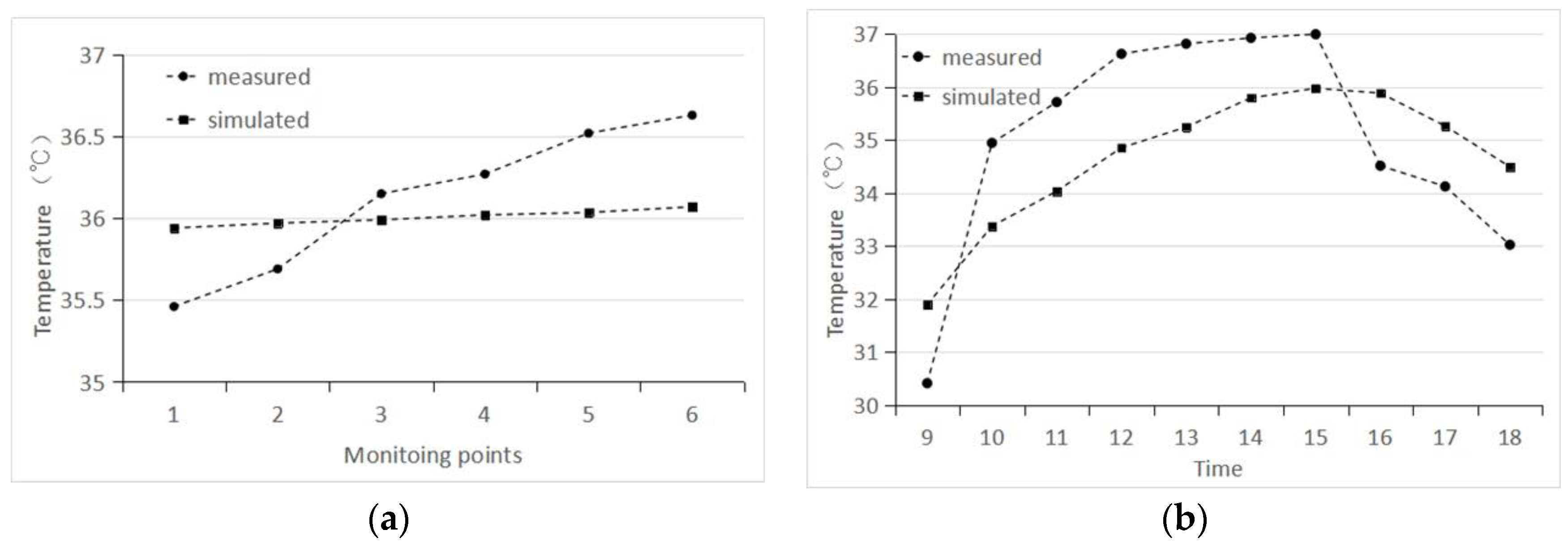
3.2. Validation of ENVI-Met Software

ENVI-met is one of the most widely used models in studies of the impact of vegetation on the outdoor thermal environment under different climatic conditions [59,60,61,62]; it is an effective simulation model. Field measurement is commonly used to verify ENVI-met. For verifying the validity of the ENVI-met model, seven monitoring points were set up in different locations of the block, in which the distances of monitoring points 1–6 from the streams were 4 m, 8 m, 12 m, 16 m, 20 m, 24 m, respectively; monitoring point 7 was selected on the open road in the regularly residential area with a parallel layout pattern (Figure 1).The selecting monitoring points 1–6 followed the criteria that these points were on the relatively open site, which was not influenced by buildings and vegetation, so as to ensure the consistency of the environment of all monitoring points, and so that the cooling effect of streams can be tested better. Based on the criteria of the six selecting points, monitoring point 7 is still selected as the seldom active site, which is not influenced by people and cars in order to reduce the measurement error. As these factors will have a certain impact on temperature measurement—the temperature of the simulation results is not affected by these factors. The task of monitoring points 1–6 was to record the temperature values at 1.5 m height at 2 p.m. while monitoring point 7 was to record the temperature at 1.5 m height from 9 a.m. to 6 p.m., recorded every 1 h. The instrument used in the field is NK5500 (Kestrel 5500) meteorological instrument, which is the most comprehensive of all the hand-held meteorological instruments of the Kestrel series, and can record up to 14 meteorological parameters such as temperature in real time. This instrument can measure in a temperature range from −29 °C to 70 °C, with precision of 1 °C and resolution of 0.1 °C, thus can meet the demands of this research.

By studying the measured and simulated values of the temperature of monitoring points 1–6 (Figure 3a), the changing trend of the two groups’ values were similar. By studying the measured values and simulated values of the temperature at monitoring point 7 (Figure 3b), the change of the simulated values was relatively smooth in the day, however, the change of the measured values displayed abrupt phenomena, which was related to the complicated reality surroundings. Uncontrollable factors in the block may lead to the change in temperature in a specific period of time, but the variation trend of the two groups’ vales by time also had similar characteristics.

On this basis, the accuracy of the model was evaluated by calculating the root mean square error (RMSE), which is commonly used at home and abroad [63,64].

$$\mathrm{RMSE}=\sqrt{\frac{{\displaystyle \sum _{\mathrm{i}=1}^{\mathrm{n}}({\mathrm{y}}_{\mathrm{i}}^{\prime }-y_i)({\mathrm{y}}_{\mathrm{i}}^{\prime }-y_i)}}{\mathrm{n}}}$$

(1)

In Formula (1), ${\mathrm{y}}_{\mathrm{i}}^{\prime }$ is the simulated value, ${\mathrm{y}}_{\mathrm{i}}$ is the measured value, and n is the measured times [65].

The RMSE between the measured and simulated values of monitoring points 1–6 and 7 is 0.45 °C and 1.43 °C, respectively. For reference to the evaluation of the ENVI-met model by other scholars, the RMSE of temperature is 1.31–1.63 °C [66], which shows that the error between the measured value and the simulated value in this paper is small and the microclimate environment can be well predicted.

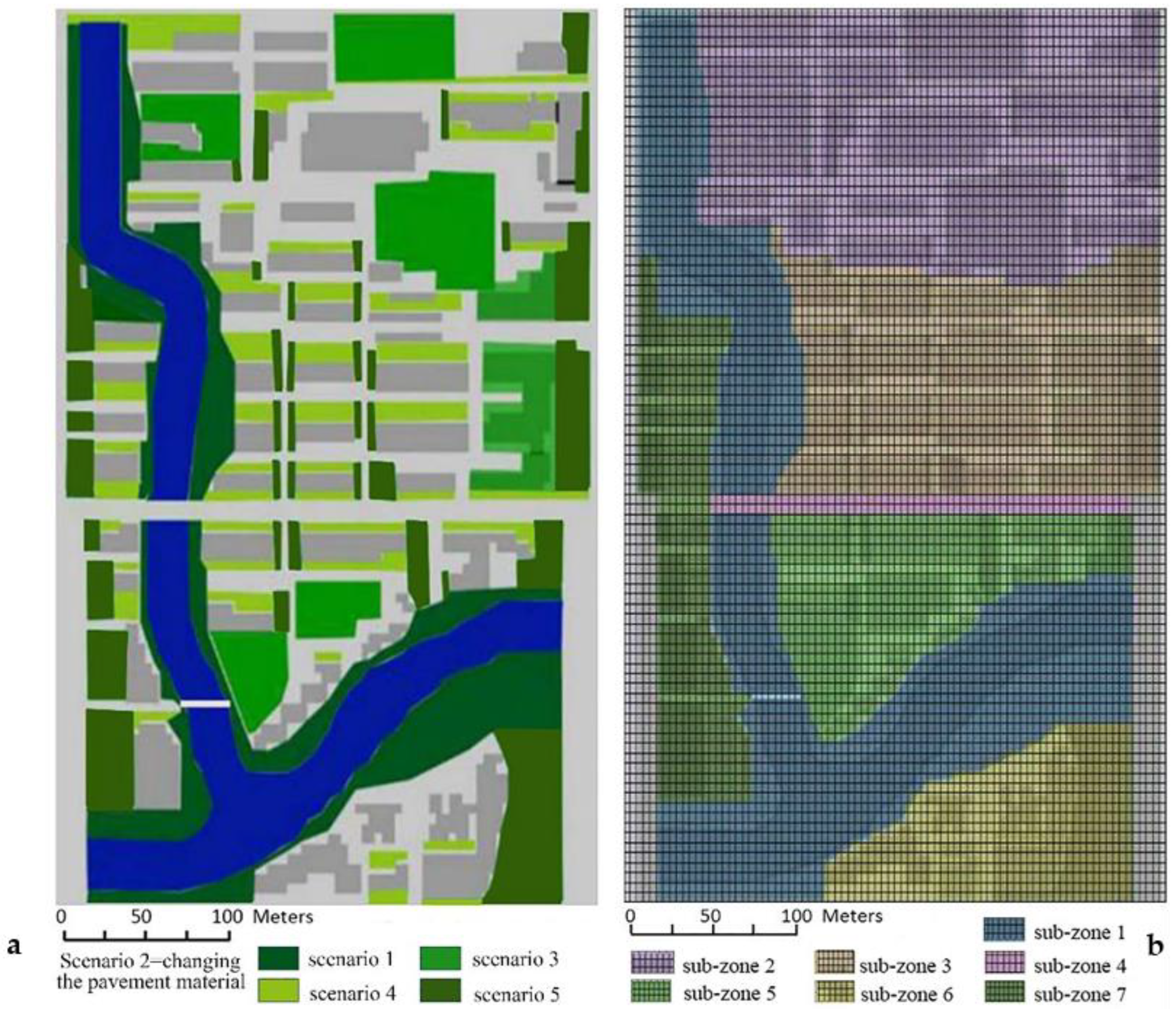
3.3. The Planning Scenarios and Spatial Subtraction Analysis

The climatic adaptive measures in site scale are mainly referred to the improvement of the vegetation forms and distribution, water resources, and urban materials [67]. Vegetation measures have shown great promise in mitigating the adverse effects of heat islands and providing superior pedestrian thermal comfort [68]. A green rate above 0.45 is essential to reduce the temperature by a maximum of 2 °C in the built environment [69]. The air temperatures in the street spaces with high-percentage canopy coverage were significantly lower than in streets with low-percentage canopy coverage [70,71]. The different green spaces with tree–shrub–herb structure, the shrub–herb structure, and pure herb structure decrease air temperature by approximately 4.8 °C, 1.3 °C, and 0.9 °C, respectively, compared with spaces with nongreen coverage [72]. For the same green-structure type, the size of the patch affects the cooling effect [73]. The highest cooling value for large patches with tree–shrub–grass compound structure is 2.8 °C, which is 0.8 °C higher than small patches with the same greening structure. The cooling value with shrub–grass structure of large patches and small patches reached a maximum of 1.4 °C and 1.2 °C, respectively [74]. Vegetation with water bodies has a synergistic cooling effect through evaporation and evapotranspiration associated with the heat transfer between water, vegetation, and air [75]. High-albedo materials in residential blocks also affect the thermal environment [76,77]. An increase in the albedo of paving material by 0.25 will reduce the temperature by 10 °C [78]. Roof vegetation also increases the albedo of the roof, thereby decreasing the amount of the absorbed solar radiation [79,80], and the fluctuation amplitude of the roof slab temperature was found to be reduced by 3 °C [81]. The cooling effects of shrubs on the roof are about twice the effect of lawn. In addition, the shadow of high buildings in the sun has a certain cooling effect [42].

Using the adaptive measures and the cooling effect results of different measures, the optimal layout of adaptation planning was put forward to form an ecological network linking landscape nodes and corridors in urban blocks. The implementation of the optimal layout of adaptation planning was divided into five parts, so five planning scenarios were designed to study the different effects of their thermal environment (Figure 4a).

Scenario 1: increasing the width of riparian green extension. We designed green corridors at least 20 m wide to form the strongest cooling-effect area from the aspect of water body impact. Combined with the actual situation of land use, the ecological landscape corridors were formed through the transformation of land use along the two sides of the two creeks, and the regions of important ecological nodes were appropriately extended to a larger scale.

Scenario 2: changing the pavement material of the residential streets. The streets in the inner residential block were replaced with high-albedo concrete.

Scenario 3: further optimizing the ecological landscape nodes. We combined the original green spaces in the study area, designed green patches with tree–shrub–herb structure instead of shrub–herb structure, and appropriately expanded rare green patches to form new landscape nodes. The maximum area of the planned landscape node is 15,072 m² and the minimum is 1680 m². Vegetation roofs were used, as the ground space in some locations could not be reformed. The vegetation roofs were made by a combination of shrubs and grass.

Scenario 4: increasing the east-west linkage of the landscape nodes by street vegetation. The vegetation width of the streets was increased as much as possible (up to 12m), thereby forming green corridors in an east-west direction and improving the connections of the landscape nodes.

Scenario 5: increasing the north-south linkage of the landscape nodes by street vegetation. The vegetation width of the landscape corridor reached 36 m at the external boundary, with a ventilation corridor with a width of more than 28 m inside the block. To improve the connection of the landscape nodes, multistory buildings in weak thermal environment areas (analyzed according to the simulation results of the residential block situation) with low-value, old buildings were transformed into sub-high-rise buildings, which also increased the shadow regions of the buildings from solar radiation.

According to the internal land use functions and the ecological boundaries and street boundaries within the residential block, the spatial pattern of the planning layout was partitioned into seven zones (Figure 4b). Subzone 1 is a natural landscape partition composed of a planning area of blue-green corridors along the two urban creeks. Subzone 2 is located on the east side of the north-south creeks; it is a mixed land partition for commercial and public functions. Subzone 3 is on the east and north sides of the two urban creeks in the residential block, and the inner main street and the green corridor of north-south creek define the boundary of the residential subzone. Subzone 3 is a residential function zone with multistory and high-rise buildings, in which the buildings to the east edge are in a semi-enclosing layout, and the residential unit buildings in the main internal are in a parallel layout. Subzone 4 is the main partition of the street area within the block, one of the main “heat sources” for the block’s thermal environment. Subzone 5 is located in the northern area, surrounded by the two urban creeks, with the downwind direction area to validate the waterside influence. The residential area is mainly composed of sub-high-rise buildings. The buildings are in parallel layout, with a partial offset arrangement of the residential units. Subzone 6 is south of the two urban creeks’ intersection area, with a mixed land use type for both commercial and residential functions. The building is a symmorphic space group layout consisting of high-rise and residential apartment buildings, and it is upwind by the waterside. Subzone 7 is located on the northwest side of the two urban creeks, with commercial and residential mixed functions. It is a long, narrow form and is a downwind subzone affected by the two creeks.

In the process of spatial analysis on the thermal environment of greening network optimization in this block, there are five steps, each of which is designed on the basis of the previous step. When the single effect of different scenarios was further analyzed, the study adapted the method of subtraction analysis, namely, the single cooling effect of the development scenario was presented by subtracting the temperature change between two scenarios at the height of 1.5 m.

4. Results and Discussion

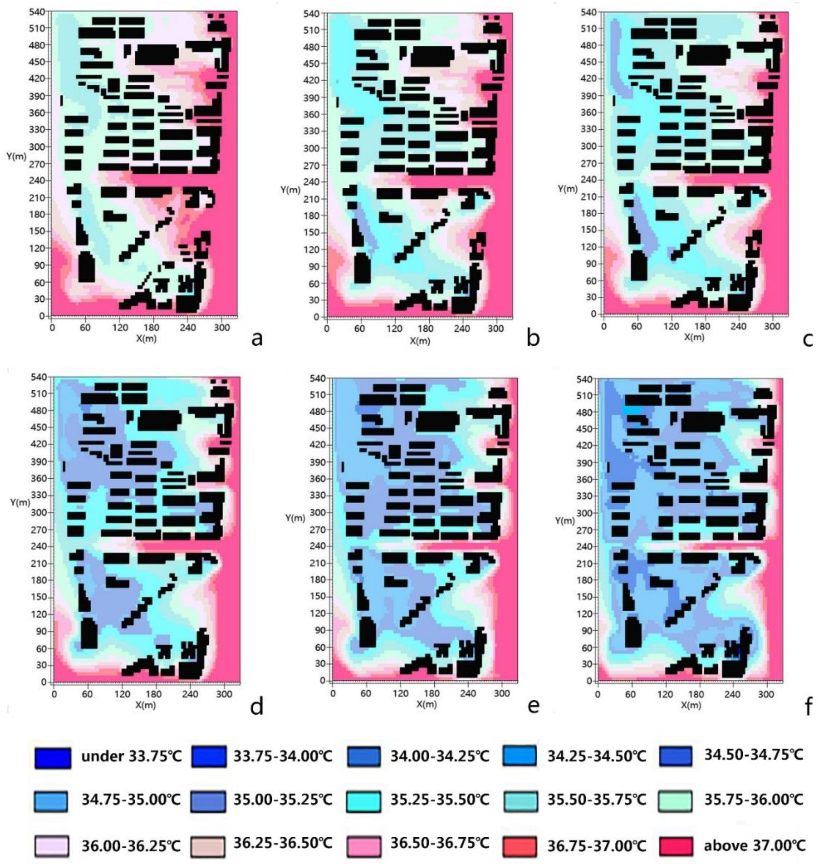
4.1. The Thermal Environment Distribution of the Current Situation

According to the regulations of the China Meteorological Administration, a daily maximum temperature reaching or exceeding 35 °C is called a high temperature, and a high temperature weather incident lasting several days (commonly more than 3 days) is called a heat wave. Since China has a vast territory and a great difference in climate zones, the China Meteorological Administration also states that various provinces and municipalities can define the threshold value of the standard of high temperature according to the local climate zone and climate characteristics [82,83]. The 35 °C standard of the National Meteorological Administration has been adopted by Shanghai [84,85]. The highest temperature in a day occurs at approximately 2 p.m., so the aim for a standard cooling effect is the 35 °C threshold at the daily time of 2 p.m.

Figure 5 shows the proportional distribution of each temperature grade in the studied residential area at 2 p.m. The temperature value under the current circumstances ranges from 35.20 °C to 38.28 °C, and the mean temperature is 36.49 °C. Based on the status of the simulated temperature distribution in the study area (Figure 3), the temperatures in the east and south are higher, whereas the temperatures in the west and north are lower, which shows that the north-south creek has a cooling effect on the surrounding areas, and this cooling effect is also obvious within the block. The southwest-northeast creek does not seem to exert a significant cooling effect, with only a small range of cooling effect at the intersection of the two creeks. Some highly dense buildings grouped far from the creek and high-rise buildings have lower temperatures, which seem to be related to shadow from buildings and the local vegetation environment.

4.1.1. The Effect of Water Bodies

Water bodies have the greatest effect on temperature reduction. To further analyze the cooling effect around a creek at different places, the monitoring points were set at the same distance from the creek bank in the upper reaches of the north-south creek and the middle and lower reaches and the southwest-northeast creek. Figure 6 shows a total of 12 h of temperature variation, from 9 a.m. to 9 p.m., at different locations of the two creeks. The temperatures located in the lower reaches of the north-south creek and the interaction reaches between the creeks were lower than those of the other reaches.

To explore the synergistic effect of water bodies and vegetation as well as the thermal effect of different vegetation configurations by the waterfront, four types of vegetation configuration in the block were selected: (1) waterfront with pure trees; (2) waterfront with a mixture of trees and herbs; (3) waterfront with herbs; and (4) waterfront without vegetation. Multiple corresponding monitoring points were selected, and the average temperature was calculated in each type of area. As shown in Figure 7a, a total of 12 h of temperature change, from 9 a.m. to 9 p.m., was obtained. The results show that the waterfronts with varying vegetation configuration types have a lower temperature than those without vegetation (Figure 7a). The differing temperature values between water bodies with without vegetation also showed a synergistic cooling effect.

To explore which type of vegetation configuration and water body had the strongest synergistic cooling effect, the temperature difference between a riparian area without vegetation and three kinds of vegetation configurations were compared, as shown in Figure 6b. In general, the changing trend of the cooling effect of the three greening types was basically the same over time: temperatures gradually rose from 9 a.m., reached their highest point at 1:00 p.m., and then slowly decreased. In particular, during the daytime, the synergistic cooling effect of the waterfront with trees was greatest, and the temperature reduction was more than 0.5 °C from 11 a.m. to 3 p.m. and was more than 0.6 °C from 12 a.m. to 1 p.m. The cooling effect of waterfront with shrubs was slightly lower than that of the mixed style. During the night, the cooling effect of a single style of vegetation was not ideal, as it decreased over time and even showed a negative value for the temperature. However, the cooling effect of a waterfront with mixed vegetation increased at 5:00 p.m., from which point, a slowdown in temperature increase occurred, which also had a good cooling effect.

4.1.2. The Effect of Green Space

(1) Green patches

Three kinds of large patches of different vegetation configurations in the block, e.g., trees, trees-herbs, and herbs, were selected to further compare the cooling effects of large patches with different vegetation configurations. The corresponding monitoring points were set for the three large patches. At the same time, monitoring points were set as benchmarks in the open space without vegetation. The temperature values of different monitoring points were recorded. A comparison of the results is shown in Figure 8.

As Figure 8a presented, from 9:00 a.m. to 3:00 p.m. the temperature in the open space with the herbs or trees was much lower than in the space without vegetation. The temperatures began to converge after 7 p.m. To further analyze the cooling effects of different vegetation types, the temperature reduction values between the open space without vegetation and different vegetation types were obtained (Figure 8b). The cooling effect during the day is as follows, in descending order: Trees > trees–herbs > herbs. The cooling effect of all of the vegetation styles reached a maximum at 2:00 p.m. and then decreased gradually. However, the cooling effect of trees or herbs in the form of a single vegetation style in an open space was negative at night, while the mixed type with trees and herbs still had a weak cooling effect.

(2) Green streets

There are also different vegetation configurations for the streets inside the block. Both sides of the green street were divided into three styles: vegetation configuration with trees, vegetation configuration with trees on one side and grass on the other side, and vegetation configuration with herbs. The street with vegetation on one side was further divided into two styles: street with trees only on one side and street with herbs on one side. To further compare the cooling effects of different green streets, the corresponding monitoring points were set among the above five types of streets. At the same time, monitoring points were also used as a benchmark in the street without vegetation on both sides. Temperature changes of different monitoring points were recorded. The comparison results are shown in Figure 9.

Figure 9a shows the changing trend of temperature over time on the six cases: trees planted on both sides of the street, herbs on one side and trees on the other side of the street, herbs on both sides of the street, trees on one side of the street, herbs on one side of the street, and no vegetation on either side of the street. The cooling effects of the green streets are shown in Figure 9b. Compared to the street without vegetation, the temperature of the streets with vegetation was lower. The cooling effect with trees on both sides of the streets was best compared to streets without vegetation. The tendency of the cooling effect of vegetation on both sides of the street was similar over time, and the tendency of the cooling effect of vegetation on only one side of the street was also similar. The cooling effect of the configuration with vegetation on both sides was better than that of the configuration with vegetation on only one side, and the cooling effect of trees was better than that of grasslands. The time segments corresponding to the highest cooling effect of different vegetation types differed, and the clear time period for the cooling effect with each type was between 10 a.m. and 2 p.m. Except for the vegetation style with herbs on both sides, the other types of green streets still played a cooling role at night.

4.2. The Comprehensive Analysis of Cooling Effect in Different Scenarios

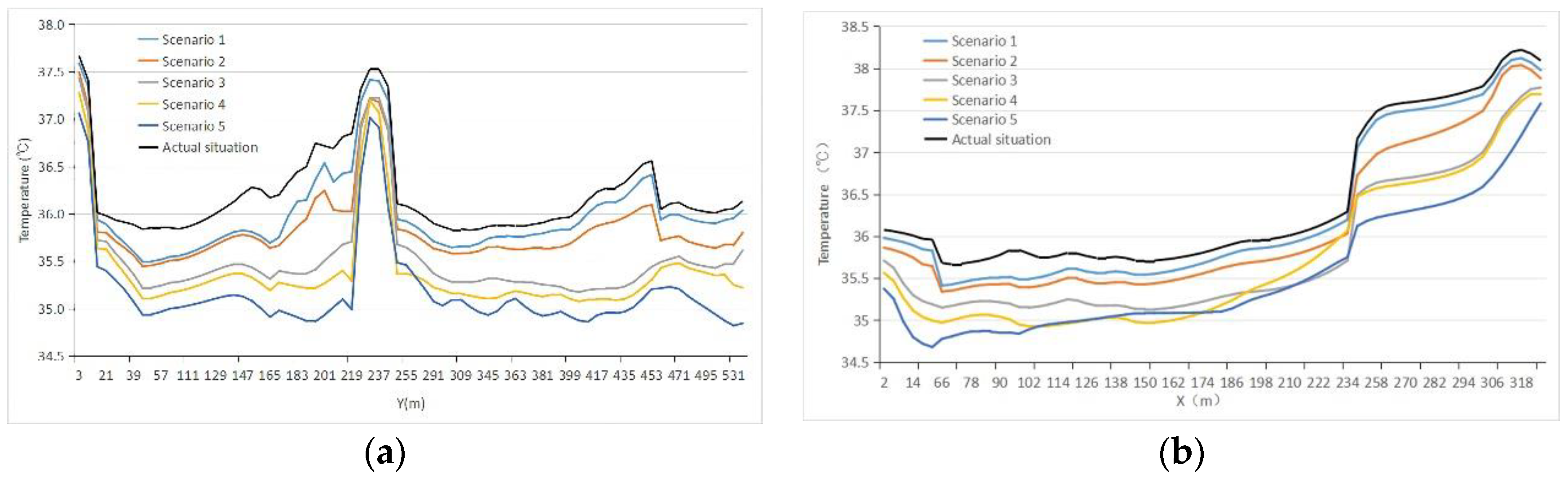
4.2.1. The Total Change of the Thermal Environment for Different Scenarios

On the basis of different planning scenarios, the greening scheme of each step was simulated, and the cooling effects were analyzed. To achieve the detailed temperature changes affected by different scenarios, the temperature range was divided into 15 grades from the original 10 grades, as shown in Figure 10.

The range of the temperature values in Scenario 1 was 35.02–38.19 °C, compared with the actual situation. The minimum temperature and maximum temperature decreased, of which the lowest temperature reduction and the highest temperature reduction were 0.18 °C and 0.09 °C, respectively. All scenarios presented a minimum temperature higher than 35 °C. Comparing the temperature spatial distribution of Figure 10a,b, the range and the intensity of lower temperature values had obviously expanded. The cooling range extended in the east-west direction, and the southwest-northeast creek with increased vegetation began to exert a cooling effect, which also indicated the coordination cooling effect of water bodies and vegetation.

The range of the temperature values in Scenario 2 was 35.02–38.12 °C. Compared with Scenario 1, the minimum temperature was same, and the maximum temperature decreased by 0.07 °C. Comparing the temperature spatial distribution of Figure 10b,c, the area of the lower range had increased in the inner area of residential groups, which showed the cooling effect of the material with higher reflectivity.

The range of the temperature values in Scenario 3 was 34.69–38.06 °C. Compared with Scenario 2, the lowest and highest temperatures both decreased: the lowest temperature decreased by 0.34 °C and the highest temperature decreased by 0.06 °C. The lowest temperature appeared below 35 °C. Comparing the temperature spatial distribution of Figure 10c with Figure 10d, the area of the lower range continued to expand, covering almost the entire block except for the occasional hot points to the northeast. Areas below 35 °C were distributed in a dotted pattern, mainly distributed near the water. The cooling functions of the larger landscape nodes were explained as being important.

The range of the temperature values in Scenario 4 was 34.51–38.02 °C, the lowest temperature and the maximum temperature were further decreased compared with the results of Scenario 3. Among these values, the lowest temperature decreased by 0.18 °C, and the highest temperature decreased by 0.04 °C. Comparing Figure 10d with Figure 10e, the high temperature range in the northeast narrowed. The coverage of temperature below 35 °C also expanded from a spotty distribution to a zonal distribution. The main inner area surrounded by the two creeks had significantly increased. The role of east-west green corridors is thus very important.

The range of the temperature values in Scenario 5 was 33.61–37.86 °C, and the lowest and highest temperatures decreased relative to earlier scenarios: the lowest temperature decreased by 0.1 °C and the highest temperature decreased by 0.16 °C. The lower temperature range in the northeast further decreased compared with the results of Scenario 4. The coverage area of temperature below 35 °C not only greatly expanded, but it also changed from zonal distribution to planar distribution, with a wide range of distribution both in the area near the creek and in the entire residential inner area. Moreover, the decreased temperature intensity was reduced by a larger margin than before, with temperatures mostly below 34.75 °C. The north-south green corridors had a significant cooling effect.

Comparing the temperature spatial distribution of the actual situation with Scenario 5, the main area in the lower temperature range expanded from a part of to nearly the whole block, and the mean temperature decreased from 36.49 °C to 35.48 °C. The percentage of temperatures below 35 °C increased from 0% to 37.81%. Figure 11 shows that the cooling effect of the residential block had been significantly improved (Figure 11), as shown by calculating the size of the area occupied by different cooling ranges. The area where the cooling range is above 0.8 °C was approximately 77%, approximately 25% of the block reached a cooling rate above 1.2 °C, and the area characterized by the cooling rate above 1.6 °C accounted for 4.45%.

4.2.2. The General Changes of the Cooling Effect with Different Scenarios

A histogram of the proportional distribution of different temperature grades at the height of 1.5 m at 2 p.m. was produced based on different simulated scenarios (Figure 12). The proportion of temperature range below 35 °C was 3.97% in Scenario 3. In Scenario 4, the proportion of temperature range below 35 °C expanded from 3.97% to 15.26%. In Scenario 5, the temperature range below 35 °C further expanded to 37.81%. The proportion of other temperature ranges also obviously changed. The proportion of the second lower temperature range, which is 35–35.3 °C, continued to increase from Scenario 1 to Scenario 4. The proportion of temperature ranges above 35.3 °C gradually decreased from Scenario 2 to Scenario 5, indicating that the proportion of higher temperatures above 35.3 °C had significantly decreased.

4.2.3. Spatial Distribution Trend of Cooling Effect from Different Scenarios

To further analyze the spatial distribution differences of the temperatures in the block, two profiles were taken from X = 180 m and Y = 270 m in the modeling grids of the residential block (Figure 13), as the selected locations had as few building shadows as possible. From the profile of X = 180 m, the temperature of the asphalt street in the block was obviously higher than that in other places, and it became the peak point. From the profile of Y = 270 m, the asphalt street’s temperatures in the eastern part of the block were above 38 °C, which was also the peak of the profile. However, the trends of temperature changes in both scenarios were consistent with the actual situation in either the east-west profile or the north-south profile, and the temperature values decreased gradually from Scenario 1 to Scenario 5.

Four kinds of surface materials, e.g., water, vegetation, concrete, and asphalt, were selected to compare their temperature differences at 2 p.m. in each step of the scenario scheme through calculating their mean temperature and standard deviations of the coverage meshes of different surface materials (Figure 14). The average temperature of each surface material decreased gradually from Scenario 1 to Scenario 5. In Scenarios 1 and 2, the temperature values of four kinds of surface materials were all above 35 °C. In Scenario 3, the surface covered by water and vegetation began to display temperature values lower than 35 °C, as shown by analyzing the standard temperature deviation of the two materials. In Scenario 4, the temperature value of the surface covered by water and vegetation as well as that of the concrete streets appeared to have areas with temperatures less than 35 °C. In Scenario 5, the area with a temperature below 35 °C decreased further for surfaces covered by water, vegetation, and concrete streets, but the minimum temperature of the asphalt streets were always higher than 35 °C.

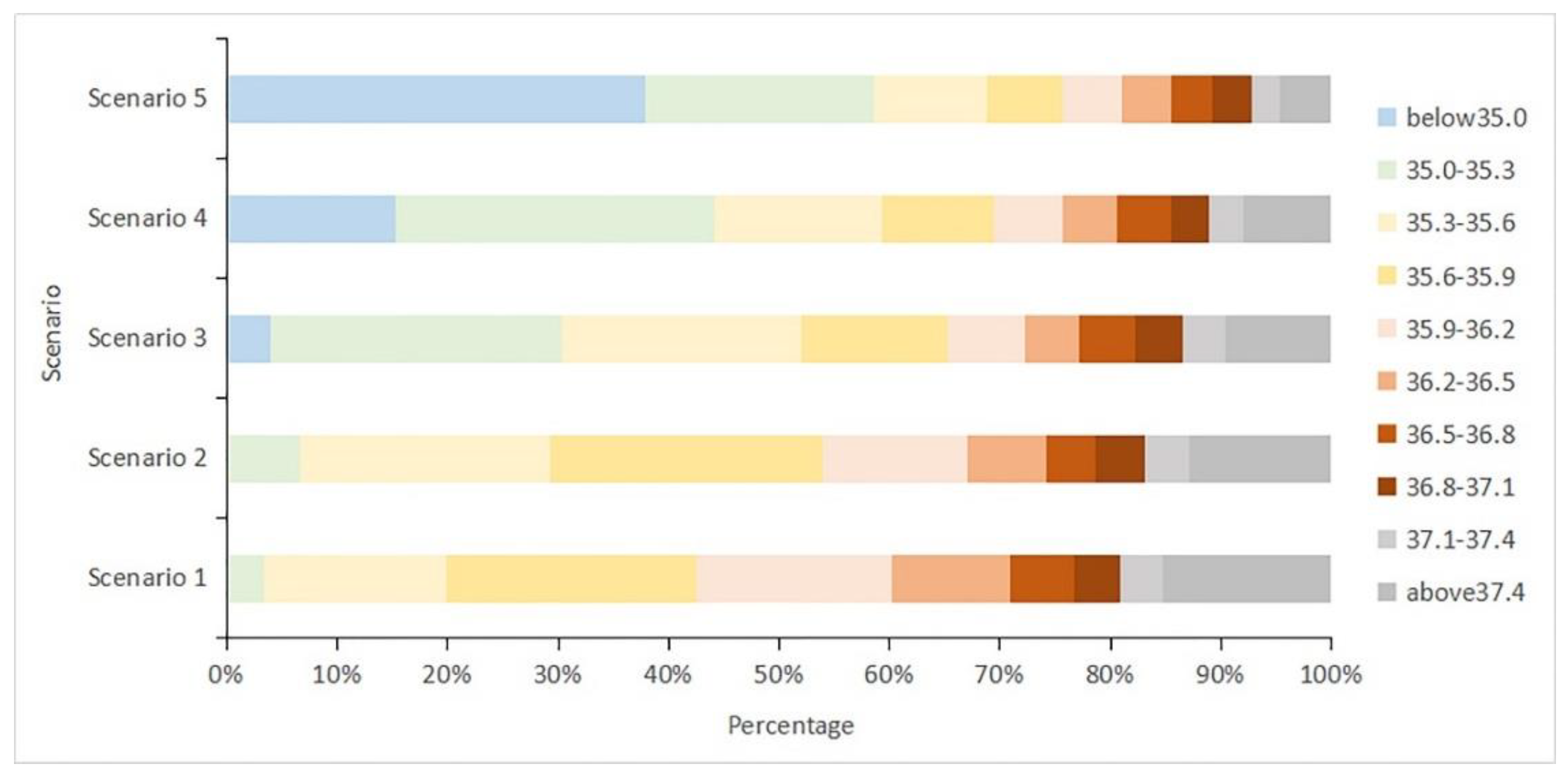
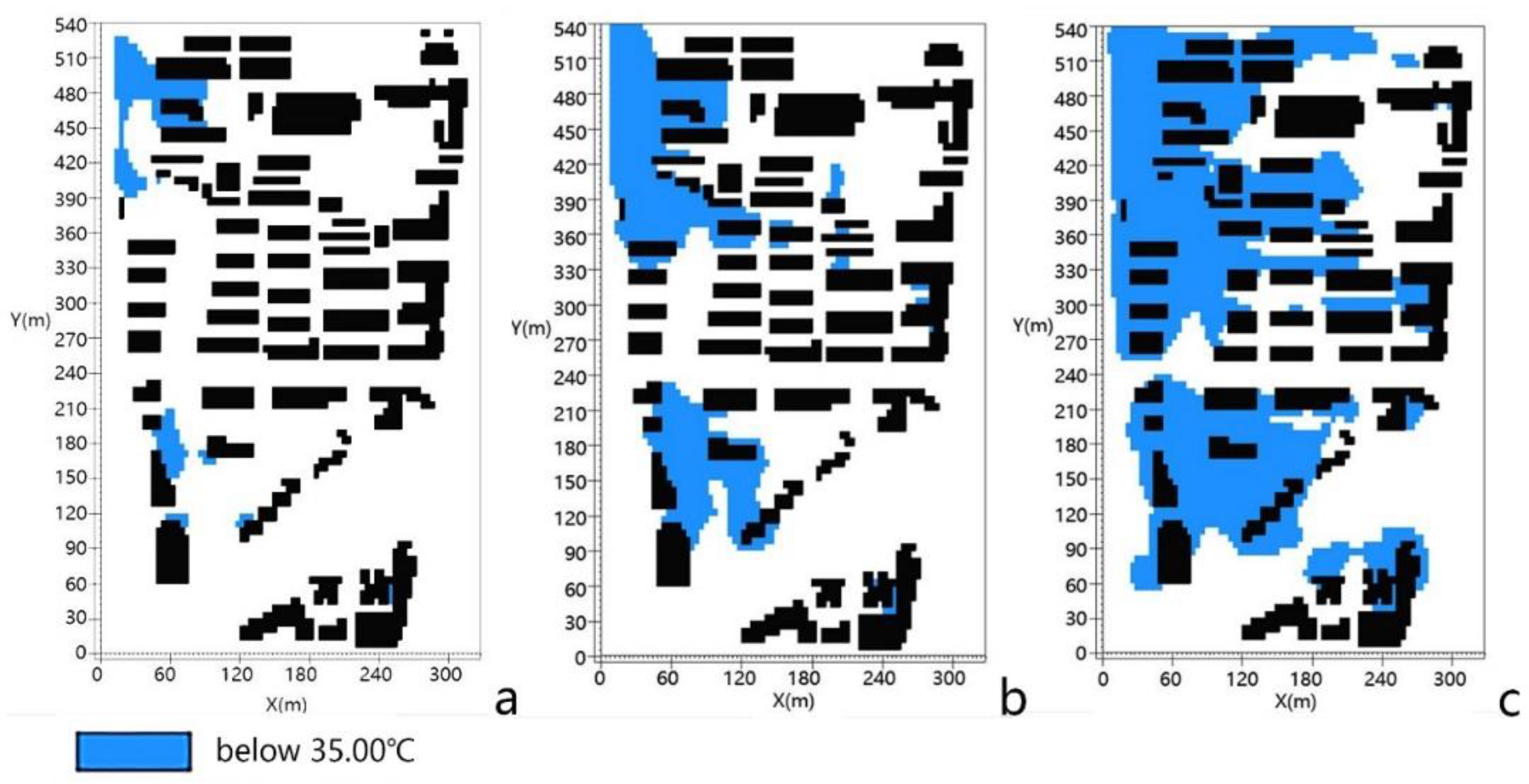
4.2.4. The Distribution Area Changes for Cooling Target Value from Different Scenarios

The preset cooling target value is to reach temperatures below 35 °C. These adaptive measures gained the cooling effect gradually and began to reach the target value in Scenario 3, Scenario 4, and Scenario 5; that is, the temperatures were below 35 °C. Figure 15 shows the range of distribution that reached the target value in these three scenarios.

Figure 15a shows that the area reaching the target temperature value was very small in Scenario 3, and the distribution appeared in the vicinity of the north-south creek and in the intersection area of the two creeks. Compared to Scenario 3, Scenario 4 had a significant increase in the area that reached the target value for cooling. Figure 15b shows that the distribution along the north-south creek broadened significantly, such that even the area at the edge of the southwest-northeast creek began to appear within the lower temperature range, and some spotty distributions with vegetation patches inside the block displayed lower temperature values. Scenario 5 shows a further increase in the area reaching the target value for cooling. Figure 15c shows that the distribution covered nearly the entire area adjacent to the two creeks and extended eastward to the inner residential groups of the block. It presented large zonal and surface distributions inside the block.

4.3. The Detailed Cooling Effect Distribution Analysis for Different Scenarios

4.3.1. The Cooling Effect of Single Spatial Structure for Different Scenarios

The analysis of different scenarios in the preceding section analyzed their synergy through different elements of the green network and determined the cooling effect intensities among different green network structure elements. Through differential thermal analysis using the LEONARDO Module of ENVI-met Software, the single cooling effect of five scenarios was simulated (Figure 16).

After subtracting the difference between Scenario 1 and the actual situation, the range of temperature difference was −1.32–0 °C, e.g., the single cooling effect of the scenario 1 was 0–1.32 °C. A certain range of areas close to the water had obvious cooling effects. The area of the north-south creek had a cooling range of 0.2–0.4 °C, which showed the distance attenuation around the north-south corridor. The cooling range of 0.4–0.6 °C was mainly distributed in the western part of the block, illustrating that the water body had great impact on surrounding areas in the downwind direction. The maximum cooling value reached 1.32 °C, near the southwest-northeast creek with a green patches in that area.

The single cooling effect of Scenario 2 was 0–0.58 °C, representing a very small alteration in cooling intensity. However, the larger open space was occupied by streets, so the adaptive measures affected the cooling processes with a large cooling range.

The single cooling effect of Scenario 3 ranged from 0–1.5 °C. The coverage of the cooling range at 0.2–0.4 °C was already a broad area. Especially in the vicinity of each node, there is a better cooling effect, which formed a large buffer with different cooling levels. The coverage of the cooling range 1.2–1.4 °C was mainly distributed in the vicinity of the greening roof, and the maximum cooling value, 1.5 °C, also appeared there. The cooling effect extended across a large buffer area to affect the inner residential area, where temperatures decreased by 0.4–0.6 °C. The maximum cooling value of the public buildings in the north subzone reached 0.8–1.2 °C.

The single cooling effect of Scenario 4 was 0–1.02 °C. There is an obvious east-west direction of the ribbon cooling effect, where the cooling range is 0.2–0.6 °C. On both sides of the wide road, the cooling range of the east-west corridor extends to the interior of the residential area, and the extended range was expansive, which also played a role in cooling the local asphalt road.

The single cooling effect of Scenario 5 was 0–1.54 °C. The cooling effect of the landscape corridor on both sides of the east-west road was more obvious and formed a long buffer strip. The maximum increase of the area reached a cooling range above 0.8 °C.

Figure 16f shows the comparison between Scenario 5 and the actual situation. The result showed that the overall cooling effect was 0–2.06 °C. There is a significant overall effect from Scenario 1 to Scenario 5, especially for the water body in the downwind direction and surrounding the large green patches.

4.3.2. The Cooling Effect of Different Subzones in the Residential Block

The average and minimum temperature values in seven partition subzones (except buildings’ inner temperature) were calculated according to the actual situation and five scenarios. Six corresponding columns in each subzone, from left to right, represented the simulated values of the actual situation, Scenario 1, Scenario 2, Scenario 3, Scenario 4, and Scenario 5, respectively. Figure 17a represents the six mean temperature values corresponding to the seven subzones. Figure 17b shows the six minimum temperature values corresponding to the seven parts; the pink indicates a minimum value above 35 °C, and the deep blue indicates a minimum value below 35 °C.

As Figure 17 shows, from Scenario 1 to Scenario 5, the mean temperature and the minimum temperature of the seven subzones, which all show a decreasing trend. The effect intensities of specific cooling factors in different zones, however, were not the same.

Subzone 1 is the water and vegetation features zone. The temperature values were the lowest for the actual situation in the seven zones. In Scenario 1, the average temperature and the minimum temperature showed a significant decrease of 0.34 °C. In Scenario 3, the minimum temperature began to fall below 35 °C. Thus, the synergistic effect of the whole green network is obviously very important and stable.

Subzone 2 had larger green patches distributed in the inner zone. Compared with the previous scenario scheme, the maximum decrease of the average temperature and the minimum temperature appeared in Scenario 3 for the buffering cooling effect of the green patches. In addition, the minimum temperature is lower than 35 °C for the same scenario measures. As the subzone is located in a downwind direction, the cooling intensity was affected by the last two steps of green corridors and network formation.

Subzone 3 showed a significant decline in the average temperature and the minimum temperature compared with the previous greening scheme in Scenario 3 and Scenario 4. As the roof vegetation on the east side of area was adapted in Scenario 3 and Scenario 4, several corridors were formed in the inner part of the subzones. Under Scenario 4 conditions, the minimum temperature began to drop below 35 °C, and in Scenario 5, the downwind area was also affected by the north-south corridors.

Subzone 4 is the asphalt street; one of the “heat sources” of the block. The average temperature and the minimum temperature were always the highest in this subzone. Compared with the previous greening scheme, the average temperature, and the minimum temperature decrease in Scenario 4 were the largest. In Scenario 5, the minimum temperature is below 35 °C, showing the integrated cooling effect of the whole green network.

Subzone 5 is also located in the downwind area surrounded by the two creeks. In Scenario 1, the average temperature and the minimum temperature were greatly decreased, the average temperature decreased by 0.37 °C, and the minimum temperature decreased by 0.48 °C. In Scenario 3, the minimum temperature was lower than 35 °C, and the green corridor network further decreased the cooling effect afterward.

Subzone 6 is adjacent to the southwest-northeastern creek, but in the upwind direction of the water features. The average temperature and the minimum temperature decreased. The most obvious decline was under the conditions of Scenario 5, in which the average temperature decreased by 0.48 °C, and the minimum temperature decreased by 1.05 °C, as affected by the large areas of green spaces and the green corridor along the external road.

Subzone 7 is adjacent to the west side of the north-south creek and the downwind area with a narrow group of buildings along the external road. As affected by the heat source of the external road, the temperatures in the whole inner zone are relatively higher than other functional zones. In Scenario 1, the average temperature and the minimum temperature also show a larger decrease in the area downwind of the water body. The decline was most significant in Scenario 5, in which the average temperature decreased by 0.52 °C, and the minimum temperature decreased by 1.05 °C, due to the cooling effect of the north-south green corridor.

5. Conclusions

To create comfortable microclimate conditions through ecological adaptation measures in a typical older residential block, ENVI-met’s numerical simulation method was used to predict the different cooling effects of spatial elements on the day of the summer solstice. The following points can be made. (1) The urban creek with a green corridor plays a significant role in the thermal cooling effect for a certain distance. The creek with a green corridor in the north-south direction had a buffering area closely connected to distance factors, and the water body in the downwind direction had a large microclimate impact on surrounding areas. (2) The highly reflective material also played a definite role in decreasing the effect of high temperatures for large areas of the residential block. (3) The cooling effect of green patches, especially larger patches, was highly influential in improving the thermal environment. The single cooling effect near the roof vegetation cannot be ignored because it supplements the cooling effect in a restricted area. (4) The effect of the east-west corridors on the improvement of the street and the surrounding space of the walking space was remarkable. It had a stable cooling effect on each area of the whole block, and linked the elements in the green space network, enhancing the cooling range of the overall space in the block. (5) The north-south corridor is the most significant element for cooling effect among all the adaptive measures. Especially under the synergistic effect of cold air sources such as bodies of water, the improvement of the thermal environment was obvious. (6) The overall green space network pattern had a greater cooling effect than did any single element in the green space network.

The ecological function of urban river corridors network is no doubt an important factor for making optimization strategy. However, the synergistic effect of utilizing green and bluespace for improving the urban thermal environment should rely on scientific research data and methods to guide the creation of rational development policies. According to the corresponding results of this research area, the cooling effect of urban creeks in residential areas is significant for mitigating UHI intensity. Landscape greenways along urban streams or creeks create an urban cold island space. Thus, as the core zones of the cooling source, the bluespace should protect and construct the control greening line for the ecological green corridor (with a lowest width of 20 m). When the urban cooling island space needs to further enhance the cooling effect, the pattern of green space network structure is very important. The cold air diffusion channel and ventilation corridor by green space network can strengthen the cooling effect to a certain extent. The layout of the north-south ventilation green corridor should be considered, which will have a good cooling effect on the downwind residential area and affect the overall thermal environment of the whole area. As for considering the synergistic effect of the blue and green infrastructure, it is suggested that residential areas adjacent to urban rivers should be constructed to set up green corridors connecting the greenway of the river, so as to form a green infrastructure system to maximize the cooling effect of residential space environment. Large-scale node of landscape ecological space has a significant mitigation effect on the thermal environment of the surrounding local space. It is very important for large-scale roof greening to improve the thermal environment of the residential block in the case of high density building area. Therefore, for making adaptive polices regarding the urban climate, the rational organization the pattern of ecological network space, and the decentralized large landscape green space at the nodes of the network are of great significance to the improvement of residential thermal environment.

In the face of complex urban block construction and the influence of the spatial elements and position elements of the urban creeks on the microclimate of the blocks, the improvement schemes require further investigation by application of the scientific principles and determination of the actual effective factors to provide better practical guidance. Dynamic predictions of a certain spatial pattern and further simulations of these scenarios, planning for microclimate effects, are also possible in further studies. For generalizing the influence features of different spatial form and structure about blue and green infrastructure on urban climate adaptation, a case study is not enough. To be able to generalize the results requires repetitions on different case areas. The way in which this paper was designed can help guide future research, and the statistically significant differences in the gradient of urban densities could be adapted in future research. These research methods will become an important part of the assessment process of future planning and design regarding site scale in cities.

References

1. IPCC. 2014: Climate Change 2014: Synthesis Report. Contribution of Working Groups I, II and III to the Fifth Assessment Report of the Intergovernmental Panel on Climate Change; Core Writing Team, Pachauri, R.K., Meyer, L.A., Eds.; IPCC: Geneva, Switzerland, 2014; p. 151. Available online: http://ar5-syr.ipcc.ch/ (accessed on 10 February 2016).
2. Huang, W.; Li, J.; Guo, Q.; Mansaray, L.; Li, X.; Huang, J. A satellite-derived climatological analysis of urban heat island over shanghai during 2000–2013. Remote Sens. 2017, 9, 641. [Google Scholar] [CrossRef]
3. Wang, J.; Yan, Z.; Quan, X.W.; Feng, J. Urban warming in the 2013 summer heat wave in eastern China. Clim. Dyn. 2017, 38, 3015–3033. [Google Scholar] [CrossRef]
4. Aflaki, A.; Mirnezhad, M.; Ghaffarianhoseini, A.; Ghaffarianhoseini, A.; Omrany, H.; Wang, Z.H.; Akbari, H. Urban heat island mitigation strategies: A state-of-the-art review on Kuala Lumpur, Singapore and Hong Kong. Cities 2017, 62, 131–145. [Google Scholar] [CrossRef]
5. Bhati, S.; Mohan, M. Wrf model evaluation for the urban heat island assessment under varying land use/land cover and reference site conditions. Theor. Appl. Climatol. 2016, 126, 385–400. [Google Scholar] [CrossRef]
6. Mcguire, A.D.; Sitch, S.; Clein, J.S.; Dargaville, R.; Esser, G.; Foley, J. Carbon balance of the terrestrial biosphere in the twentieth century: Analyses of co2, climate and land use effects with four process-based ecosystem models. Glob. Biogeochem. Cycles 2001, 55, 183–206. [Google Scholar] [CrossRef]
7. Shi, P.; Yi, Y.; Jin, C. The effect of land use on runoff in Shenzhen city of china. Acta Ecol. Sin. 2001, 2121, 1041–1049. [Google Scholar]
8. Zibibulla, S.; Zhang, Y.F.; Yin, Z.G.; Zhang, J.; Paxiagu; Suliye; Zumiret. Relevance Analysis between Urbanization and Urban Land Use Change of Korla City. Xinjiang Agric. Sci. 2010, 4747, 1025–1029. [Google Scholar]
9. Hara, Y.; Takeuchi, K.; Okubo, S. Urbanization linked with past agricultural landuse patterns in the urban fringe of a deltaic Asian mega-city: A case study in Bangkok. Landsc. Urban Plan. 2005, 7373, 16–28. [Google Scholar] [CrossRef]
10. Lee, Y.Y.; Din, M.F.M.; Ponraj, M.; Noor, Z.Z.; Iwao, K.; Chelliapan, S. Overview of urban heat island (uhi) phenomenon towards human thermal comfort. Environ. Eng. Manag. J. 2017, 1616, 2097–2112. [Google Scholar]
11. Sang, Y.F. Wavelet entropy-based investigation into the daily precipitation; variability in the Yangtze river delta, china, with rapid urbanizations. Theor. Appl. Climatol. 2013, 111, 361–370. [Google Scholar] [CrossRef]
12. Zhu, Z.; Zheng, B. Study on spatial structure of Yangtze river delta urban agglomeration and its effects on urban and rural regions. J. Urban Plan. Dev. 2012, 138, 78–89. [Google Scholar]
13. Xiong, Y.; Huang, S.; Chen, F.; Ye, H.; Wang, C.; Zhu, C. The impacts of rapid urbanization on the thermal environment: A remote sensing study of Guangzhou, China. Remote Sens. 2012, 44, 2033–2056. [Google Scholar] [CrossRef]
14. Huang, Q.; Lu, Y. The effect of urban heat island on climate warming in the Yangtze river delta urban agglomeration in China. Int. J. Environ. Res. Public Health 2015, 12, 8773–8789. [Google Scholar] [CrossRef] [PubMed]
15. Zhang, Y.; Bao, W.J.; Yu, Q.; Ma, W.C. Seasonal variation and interannual difference of heat island effect in mega-cities. J. Geophys. 2012, 55, 1121–1128. [Google Scholar]
16. Giorgio, G.A.; Ragosta, M.; Telesca, V. Application of a multivariate statistical index on series of weather measurements at local scale. Measurement 2017, 112, 61–66. [Google Scholar] [CrossRef]
17. Kundu, S.; Khare, D.; Mondal, A. Individual and combined impacts of future climate and land use changes on the water balance. Ecol. Eng. 2017, 105, 42–57. [Google Scholar] [CrossRef]
18. Evans, E.; McGregor, G.R.; Petts, G.E. River energy budgets with special reference to river bed processes. Hydrol. Process. 1998, 12, 575–595. [Google Scholar] [CrossRef]
19. Caissie, D. The thermal regime of rivers: A review. Freshw. Biol. 2006, 51, 1389–1406. [Google Scholar] [CrossRef]
20. Gunawardena, K.R.; Wells, M.J.; Kershaw, T. Utilising green and bluespace to mitigate urban heat island intensity. Sci. Total Environ. 2017, 584–585, 1040–1055. [Google Scholar] [CrossRef] [PubMed]
21. Gu, R.; Montgomery, S.; Austin, T.A. Quantifying the effects of stream discharge on summer river temperature. Hydrol. Sci. J. 1998, 43, 885–904. [Google Scholar] [CrossRef] [Green Version]
22. Zhu, C.; Li, S.; Ji, P.; Ren, B.; Li, X. Effects of the different width of urban green belts on the temperature and humidity. Acta Ecol. Sin. 2011, 31, 383–394. [Google Scholar]
23. Hathway, E.A.; Sharples, S. The interaction of rivers and urban form in mitigating the urban heat island effect: A UK case study. Build. Environ. 2012, 58, 14–22. [Google Scholar] [CrossRef]
24. Steeneveld, G.J.; Koopmans, S.; Heusinkveld, B.G.; Theeuwes, N.E. Refreshing the role of open water surfaces on mitigating the maximum urban heat island effect. Landsc. Urban Plan. 2014, 121, 92–96. [Google Scholar] [CrossRef]
25. Theeuwes, N.E.; Solcerová, A.; Steeneveld, G.J. Modeling the influence of open water surfaces on the summertime temperature and thermal comfort in the city. J. Geophys. Res. Atmos. 2013, 118, 8881–8896. [Google Scholar] [CrossRef] [Green Version]
26. O’Malley, C.; Piroozfar, P.; Farr, E.R.P.; Pomponi, F. Urban heat island (uhi) mitigating strategies: A case-based comparative analysis. Sustain. Cities Soc. 2015, 19, 222–235. [Google Scholar] [CrossRef]
27. Mou, I.Z.H.; Fahim, M.R. Relevance of Waterbody in Inducing Low Temperature in Residential Neighborhood: A Case of Dhanmondi, Dhaka. J. Modern Sci. Technol. 2013, 1, 157–166. [Google Scholar]
28. Syafii, N.I.; Ichinose, M.; Wong, N.H.; Kumakura, E.; Jusuf, S.K.; Chigusa, K. Experimental study on the influence of urban water body on thermal environment at outdoor scale model. Procedia Eng. 2016, 169, 191–198. [Google Scholar] [CrossRef]
29. Yoon, J.O.; Chen, H.; Ooka, R.; Kato, S.; Hsieh, C.M.; Ishizaki, R.; Miisho, K.; Kudoh, R. Design of the Outdoor Thermal Environment for a Sustainable Riverside Housing Complex Using a Coupled Simulation of cfd and Radiation Transfer. Available online: http://www.irbnet.de/daten/iconda/CIB8099.pdf (accessed on 5 September 2017).
30. Lu, Y.M.; Wang, X.; Zhou, H.C. Numerical simulation of the adjustment Mechanism of water pond on microclimate in residential districts. Build. Sci. 2015, 31, 101–107. [Google Scholar]
31. Zhou, H.C. Research on Local Climate Regulated by Water Pond in Residential Area. Master’s Thesis, Guangdong University of Technology, Guangzhou, China, 2014. [Google Scholar]
32. Inard, C.; Groleau, D.; Musy, M. Energy balance study of water ponds and its influence on building energy consumption. Build. Serv. Eng. Res. Technol. 2003, 25, 171–182. [Google Scholar] [CrossRef]
33. Zhang, X.C. Study on the Thermal Environment of Water-Shore Residence in Shenyang City. Master’s Thesis, Shenyang Architecture University, Shenyang, China, 2011. [Google Scholar]
34. Wu, Z.; Kong, F.; Wang, Y.; Sun, R.; Chen, L. The impact of greenspace on thermal comfort in a residential quarter of Beijing, China. Int. J. Environ. Res. Public Health 2016, 13, 1217. [Google Scholar] [CrossRef] [PubMed]
35. Herath, H.M.P.I.K.; Halwatura, R.U.; Jayasinghe, G.Y. Evaluation of green infrastructure effects on tropical Sri Lankan urban context as an urban heat island adaptation strategy. Urban For. Urban Green. 2018, 29, 212–222. [Google Scholar] [CrossRef]
36. Ghani, A.N.A.; Ariffin, J.; Tukiran, J. A study on the cooling effects of greening for improving the outdoor thermal environment in Penang Malaysia. Int. J. GEOMATE 2017, 12, 62–70. [Google Scholar]
37. Srivanit, M.; Hokao, K. Evaluating the cooling effects of greening for improving the outdoor thermal environment at an institutional campus in the summer. Build. Environ. 2013, 66, 158–172. [Google Scholar] [CrossRef]
38. Lee, H.; Mayer, H.; Chen, L. Contribution of trees and grasslands to the mitigation of human heat stress in a residential district of Freiburg, southwest Germany. Landsc. Urban Plan. 2016, 148, 37–50. [Google Scholar] [CrossRef]
39. Abreu-Harbich, L.V.D.; Labaki, L.C.; Matzarakis, A. Effect of tree planting design and tree species on human thermal comfort in the tropics. Landsc. Urban Plan. 2015, 138, 99–109. [Google Scholar] [CrossRef]
40. Zheng, S.; Zhao, L.; Li, Q. Numerical simulation of the impact of different vegetation species on the outdoor thermal environment. Urban For. Urban Green. 2016, 18, 138–150. [Google Scholar] [CrossRef]
41. Liu, Y.; Guo, J.; Wei, Q. Urban green space landscape patterns and thermal environment investigations based on computational fluid dynamics. Acta Ecol. Sin. 2012, 32, 1951–1959. [Google Scholar]
42. Peng, L.L.H.; Jim, C.Y. Green-roof effects on neighborhood microclimate and human thermal sensation. Energies 2013, 6, 598–618. [Google Scholar] [CrossRef] [Green Version]
43. Xuan, C.Y. Impact of Water Distribution on Atmospheric Environment in Urban Area. Mater’s Thesis, Lanzhou University, Lanzhou, China, 2011. [Google Scholar]
44. Li, C.; Yu, C.W. Mitigation of urban heat development by cool island effect of green space and water body. Lect. Notes Electr. Eng. 2014, 261, 551–561. [Google Scholar]
45. Huttner, S.; Bruse, M.; Dostal, P. Using ENVI-Met to Simulate the Impact of Global Warming on the Micro Climate in Central European Cities. Available online: https://www.researchgate.net/publication/237304053 (accessed on 3 March 2013).
46. Toparlar, Y.; Blocken, B.; Vos, P.; Heijst, G.J.F.V.; Janssen, W.D.; Hooff, T.V.; Montazeri, H.; Timmermans, H.J.P. CFD simulation and validation of urban microclimate: A case study for Bergpolder Zuid, Rotterdam. Build. Environ. 2015, 83, 79–90. [Google Scholar] [CrossRef] [Green Version]
47. Langer, I.; Sodoudi, S.; Cubasch, U. Using the ENVI-met program to simulate the micro climate in new town Hashtgerd. In Proceedings of the International Conference on Computing, Networking and Digital Technologies, Sanad, Bahrain, 11–13 November 2012; pp. 61–64. [Google Scholar]
48. Ebrahimnejad, R.; Noori, O.; Deihimfard, R. Mitigation potential of green structures on local urban microclimate using ENVI-met model. Int. J. Urban Sustain. Dev. 2017, 9, 274–285. [Google Scholar] [CrossRef]
49. Salata, F.; Golasi, I.; Vollaro, A.D.L.; Vollaro, R.D.L. How high albedo and traditional buildings’ materials and vegetation affect the quality of urban microclimate. A case study. Energy Build. 2015, 99, 32–49. [Google Scholar] [CrossRef]
50. Yang, F.; Lau, S.S.Y.; Qian, F. Summertime heat island intensities in three high-rise housing quarters in inner-city shanghai china: Building layout, density and greenery. Build. Environ. 2010, 45, 115–134. [Google Scholar] [CrossRef]
51. Shanghai Statistics Bureau, Shanghai Investigation Team of National Statistics Bureau. Shanghai Statistical Yearbook 2006–2015; China Statistics Press: Beijing, China. Available online: http://www.stats-sh.gov.cn/tjnj/zgsh/nj2011.html (accessed on 12 May 2017).
52. Ministry of Commerce of the People’s Republic of China. The Rate of Urbanization in Shanghai Ranks First in the China. [EB/OL]. Available online: http://www.mofcom.gov.cn/article/resume/n/201408/20140800682921.shtml (accessed on 1 June 2017).
53. Zhao, M.; Cai, H.; Qiao, Z.; Xu, X. Influence of urban expansion on the urban heat island effect in shanghai. Int. J. Geogr. Inf. Syst. 2016, 30, 2421–2441. [Google Scholar] [CrossRef]
54. Xia, J.; Tu, K.; Yan, Z.; Qi, Y. The super-heat wave in eastern china during July–August 2013: A perspective of climate change. Int. J. Climatol. 2016, 36, 1291–1298. [Google Scholar] [CrossRef]
55. Du, Z.H.; Mo, Y.; Li, T.T. Heat wave-related excess mortality assessment in Shanghai, in summer 2013. J. Environ. Health 2014, 9, 757–760. [Google Scholar]
56. Weather Underground. Available online: https://www.wunderground.com/weather/cn/xuhui-district (accessed on 23 July 2016).
57. Shanghai Municipal Government. [EB/OL]. Available online: http://www.shanghai.gov.cn/nw2/nw2314/nw2319/nw12344/u26aw50743.html (accessed on 13 December 2016).
58. Huttner, S.; Bruse, M. Numerical modeling of the urban climate—A preview on ENVI-met 4.0. In Proceedings of the 7th International Conference on Urban Climate ICUC-7, Yokohama, Japan, 29 June–3 July 2009. [Google Scholar]
59. Salata, F.; Golasi, I.; Vollaro, R.D.L.; Vollaro, A.D.L. Urban microclimate and outdoor thermal comfort. A proper procedure to fit envi-met simulation outputs to experimental data. Sustain. Cities Soc. 2016, 26, 318–343. [Google Scholar] [CrossRef]
60. Zhan, H.J.; Xie, W.J.; Sun, H.; Huang, H.G. Simulation of temperature distribution in 3D vegetation scene with ENVI-met model. J. Beijing For. Univ. 2014, 36, 64–74. [Google Scholar]
61. Song, B.G.; Park, K.H.; Jung, S.G. Validation of ENVI-met model with in situ measurements considering spatial characteristics of land use types. J. Korean Assoc. Geogr. Inf. Stud. 2014, 17, 156–172. [Google Scholar] [CrossRef]
62. Emmanuel, R.; Fernando, H. Urban heat islands in humid and arid climates: Role of urban form and thermal properties in Colombo, Sri Lanka and Phoenix, USA. Clim. Res. 2017, 34, 241–251. [Google Scholar] [CrossRef]
63. Middel, A.; Häb, K.; Brazel, A.J.; Martin, C.A.; Guhathakurta, S. Impact of urban form and design on mid-afternoon microclimate in phoenix local climate zones. Landsc. Urban Plan. 2014, 122, 16–28. [Google Scholar] [CrossRef]
64. Liu, Z.X.; Zheng, S.L.; Fang, X.S.; Lu, X.H.; Zhao, L.H. Simulating validation of ENVI-met vegetation model to Ficus microcarpa in hot-humid region of subtropical zone. J. Beijing For. Univ. 2018, 3, 1–12. [Google Scholar]
65. Chai, T.; Draxler, R.R. Root mean square error (rmse) or mean absolute error (mae). Geosci. Model Dev. Discuss. 2014, 7, 1247–1250. [Google Scholar] [CrossRef]
66. Chow, W.T.L.; Pope, R.L.; Martin, C.A.; Brazel, A.J. Observing and modeling the nocturnal park cool island of an arid city: Horizontal and vertical impacts. Theor. Appl. Climatol. 2011, 103, 197–211. [Google Scholar] [CrossRef]
67. Gan, Y.; Liang, T.; Chen, K.; He, R. Characteristics of the Microclimate in Residential Areas of the Different Building and Green Layout. Clim. Chang. Res. Lett. 2016, 5, 247–257. [Google Scholar]
68. Wu, Y.Y.; Zhang, X.Y.; Lei, J.L.; Zhong, L. The effects on temperature and humidity of different types of residential green-lands in Shenzhen. Guangdong Landsc. Archit. 2008, 6, 010. [Google Scholar]
69. Chandramathy, A.I.; Arch, M. Green space factor in modifying the microclimates in a neighbourhood: Theory and Guidelines. In Proceedings of the 30th International PLEA Conference, Ahmedabad, India, 16–18 December 2014; pp. 1–9. [Google Scholar]
70. Sanusi, R.; Johnstone, D.; May, P.; Livesley, S.J. Street orientation and side of the street greatly influence the microclimatic benefits street trees can provide in summer. J. Environ. Qual. 2016, 45, 167. [Google Scholar] [CrossRef] [PubMed]
71. Ouldboukhitine, S.E.; Belarbi, R.; Sailor, D.J. Experimental and numerical investigation of urban street canyons to evaluate the impact of green roof inside and outside buildings. Appl. Energy 2014, 114, 273–282. [Google Scholar] [CrossRef]
72. Li, H.; Zhao, W.Z.; Gu, R.Z.; Li, Y.M.; Chen, Z.X.; Zhang, X.X. Effects of three different green lands in plantation structure on the O2-emitting, CO2-fixing, heat absorbing and temperature decreasing in residential quarters. Environ. Sci. 1999, 6, 41–44. [Google Scholar]
73. Gál, C.V. The influence of built form and vegetation on the canopy layer microclimate within urban blocks. Acta Climatol. Chorol. Univ. Szeged 2014, 47–48, 43–52. [Google Scholar]
74. Gao, K.; Qin, J.; Song, K.; Hu, Y.H. Fallen temperature effects at green patches of urban residential areas and analysis of its influence factors. J. Plant Resour. Environ. 2009, 18, 50–55. [Google Scholar]
75. Zhang, P.; Zhang, X.; Ma, Z. Numerical simulation on the effect of river system to thermal environment of residential neighborhood. J. Shenyang Jianzhu Univ. 2010, 26, 1172–1176. [Google Scholar]
76. Erell, E.; Pearlmutter, D.; Boneh, D.; Kutiel, P.B. Effect of high-albedo materials on pedestrian heat stress in urban street canyons. Urban Clim. 2014, 10, 367–386. [Google Scholar] [CrossRef]
77. Lobaccaro, G.; Acero, J.A. Comparative analysis of green actions to improve outdoor thermal comfort inside typical urban street canyons. Urban Clim. 2015, 14, 251–267. [Google Scholar] [CrossRef]
78. Akbari, H.; Pomerantz, M.; Taha, H. Cool surfaces and shade trees to reduce energy use and improve air quality in urban areas. Sol. Energy 2001, 70, 295–310. [Google Scholar] [CrossRef]
79. Sfakianaki, A.; Pagalou, E.; Pavlou, K.; Santamouris, M.; Assimakopoulos, M.N. Theoretical and experimental analysis of the thermal behaviour of a green roof system installed in two residential buildings in Athens, Greece. Int. J. Energy Res. 2009, 33, 1059–1069. [Google Scholar] [CrossRef]
80. Zinzi, M.; Agnoli, S. Cool and green roofs. An energy and comfort comparison between passive cooling and mitigation urban heat island techniques for residential buildings in the mediterranean region. Energy Build. 2012, 55, 66–76. [Google Scholar] [CrossRef]
81. Samer, M. Towards the implementation of the green building concept in agricultural buildings: A literature review. Agric. Eng. Int. CIGR J. 2013, 15, 25–46. [Google Scholar]
82. Cheng, M.; Geng, F.H.; Ma, L.M.; Zhou, W.D.; Shi, H.; Ma, J.H. Analyses on the heat wave events in Shanghai recent 138 years. Plateau Meteorol. 2013, 32, 597–607. [Google Scholar]
83. Xu, J.F.; Deng, Z.Y.; Chen, M. A summary of studying on characteristics of high temperature and heat wave damage in China. Arid Meteorol. 2009, 27, 163–167. [Google Scholar]
84. Shi, J.; Cui, L.L.; Tian, Z. Climate characteristics of high and low temperature and its effecting factors in Shanghai. Resour. Environ. Yangtze Basin 2009, 18, 1143–1148. [Google Scholar]
85. Shi, J.; Ding, Y.H.; Cui, L.L. Climatic characteristics and their changing law during summer high-temperature times in East China. Acta Geogr. Sin. 2008, 63, 237–246. [Google Scholar]
Figure 1. Simulation domain in Shanghai. Source: Map World, 2015.
Sustainability 10 03189 g001
Figure 2. The three-dimensional model diagram and the spatial distribution in the study area by ENVI-met simulation. (a) Actual three-dimensional model and (b) spatial distribution of air temperature.
Sustainability 10 03189 g002
Figure 3. The comparison of measured temperature and simulated temperature between monitoring points 1–6 at 2 p.m. (a) and the comparison of measured temperature and simulated temperature from 9 a.m. to 6 p.m. at monitoring point 7 (b).
Sustainability 10 03189 g003
Figure 4. The planned greening network pattern and the partitioned subzones in the study area. (a) The scenarios of the green network pattern; (b) The partitioned subzones with natural elements and internal land use functions.
Sustainability 10 03189 g004
Figure 5. The proportional distribution of different temperature grades in the study area at 2 p.m.
Sustainability 10 03189 g005
Figure 6. The hourly temperature change comparisons in the upper, middle, and lower reaches of the two creeks, at the height of 1.5 m, from 9 a.m. to 9 p.m. (a) North-south creek; (b) Southwest-northeast creek.
Sustainability 10 03189 g006
Figure 7. The hourly temperature change comparison, from 9 a.m. to 9 p.m., at the waterfront with different vegetation configurations at the height of 1.5 m. (a) The temperature comparisons of four conditions; (b) the cooling values with the baseline of nonvegetation condition.
Sustainability 10 03189 g007
Figure 8. The hourly temperature changes of the open space, from 9 a.m. to 9 p.m., with different vegetation configurations at the height of 1.5 m. (a) The temperature comparisons of four conditions; (b) cooling values with the baseline of nonvegetation condition.
Sustainability 10 03189 g008
Figure 9. The hourly temperature changes of the green streets, from 9 a.m. to 9 p.m., with different vegetation configurations at the height of 1.5 m. (a) Temperature comparisons of six conditions; (b) cooling values with the baseline of nonvegetation condition.
Sustainability 10 03189 g009
Figure 10. Simulation results for different scenarios. (a) Actual situation; (b) Scenario 1; (c) Scenario 2; (d) Scenario 3; (e) Scenario 4; (f) Scenario 5.
Sustainability 10 03189 g010
Figure 11. The proportions of different decreased temperature levels after comprehensive planning for the residential block.
Sustainability 10 03189 g011
Figure 12. The proportional distribution of different temperature grades with Scenarios 1 to 5 at 2 p.m.
Sustainability 10 03189 g012
Figure 13. The profile temperature charts at the horizontal coordinate of 180 m and the vertical coordinate of 270 m of the modeling grid at 2:00 p.m. (a) The profile at horizontal coordinate 180 m; (b) the profile at vertical coordinate 270 m.
Sustainability 10 03189 g013
Figure 14. The mean temperature and standard deviation of different surface materials at 2 p.m. for Scenarios 1 to 5.
Sustainability 10 03189 g014
Figure 15. The distribution of Scenarios 3, 4, and 5 for cooling to reach below the target preset value. (a) Scenario 3; (b) Scenario 4; (c) Scenario 5.
Sustainability 10 03189 g015
Figure 16. The single cooling effect map of Scenarios 1–5 at a height of 1.5 m at 2 p.m. (a) Scenario 1; (b) Scenario 2; (c) Scenario 3; (d) Scenario 4; (e) Scenario 5; (f) comprehensive cooling effect map for Scenarios 1–5.
Sustainability 10 03189 g016
Figure 17. The mean temperature and the minimum temperature of the actual situation and Scenarios 1–5 at 2 p.m. in 7 partition subzones. (a) The mean temperature; (b) the minimum temperature.
Sustainability 10 03189 g017