1. Introduction
In recent years, researchers have suggested various empirical evidence of the cause, progress and contagion of the global financial crisis in 2007–2009. It is a well-known fact that the origin of the crisis was the downfall of the U.S. sub-prime mortgage products emanating from the collapse of the bubble in the U.S. real estate market. The burst of the bubble, which caused the collapse of its financial system, generated the depression of the world-wide real economy and the default of global firms. Although the risk of bubble and sub-prime mortgage products had been warned even before the crisis, this had not received much attention. The quantitative easing brought the stability of the U.S. economy back, but a similar bubble-related crisis may recur at any time in any country. Especially, developing countries that have experienced a rapid economic growth and expansion of the real estate market should learn the lessons from the U.S. sub-prime mortgage crisis. Indeed, around 1997, many Asian countries experienced foreign exchange crises caused by rapid internationalization of their immature financial system, which accompanied the collapse of the real estate market. In particular, as a large portion of the national economy relies on the real estate market, many researchers in developing countries have focused on discovering relationships between the economic growth and real estate market [
1,
2,
3].
Providing the information of the bubble is important to prevent the real estate-driven crisis at the market level. Currently, the Korean government publicly offers numerous indicators, but it is difficult for market participants to extract the bubble-related information from the indicators. Therefore, the purpose of this research is to propose a mathematical framework to measure bubbles in the Korean real estate market using a real options model. Through the Korean War, rapid economic development and the foreign exchange crisis, the Korean real estate market has shown sound and steady growth. Although it had been suppressed and suffered temporary downturns, the price of the Korean real estate market has continuously risen without a major price drop. The rise in price supported by economic development and real demand of housing is not problematic, but the speculation-driven rise of price without a residential demand can create bubbles in the market. Furthermore, as shown in history, bubbles in the market have a potential of causing its collapse. In this context, Kim and Suh (1993) addressed the risk of the bubble in the Korean real estate market where the major policy of the Korean government has focused on maintaining its sustainable growth [
4]. Specifically, the collapse of house prices can be catastrophic to the real economy in Korea such as the long-term recession in Japan, well-known as the Lost Decade. However, from various historical evidence, the effectiveness of any government-driven policy is questionable after the realization of the crisis. That is, the risk of bubbles in the Korean real estate market should be monitored and managed through the market equilibrium mechanism in real time. Therefore, the value of the proposed framework lies in its assistance in the reflection of the bubble-related information by market participants, which expect a more gradual effect to the stable and sustainable growth of the real estate market.
The proposed framework is designed to obtain the information of bubbles in the real estate market. In order to achieve the main objective, we incorporate the unique housing mechanism in Korea, called the Jeonse deposit system (Jeonse), also known as the key money deposit, to extract the information of the bubble from the market indices. A Jeonse contract comprises a tenant delivering a large sum of deposit, a key money deposit, to a landlord when a contract is approved. The total amount of deposit, protected by a lien issued against the property, depends on the regions, type of housing and the economy based on the ground rule. The tenant can physically possesses the property during the contract, the legally guaranteed period of which for tenant is usually one or two years. Note that the terminating condition of the contract can be the expiration date or the participants’ agreement on an early exercise. The entire deposit is re-delivered to the tenant at the end of the contract. The Jeonse was created as a way to satisfy the demand of owning a house during a period of rapid economic development with high standard interest rates. A Jeonse tenant can secure a stable residence during the contract regardless of fluctuation of house price, whereas a Jeonse landlord can expect the profits from the high interests or investments on the large sum of deposit. In particular, the Jeonse has been more active than the rental market because of the preference in long-term stable residence among Koreans. Therefore, depending on the condition of the economy, the movements of the house and Jeonse prices affect and interact with each other. A Jeonse price is an equilibrium price given that it is the maximum price for a tenant’s residential needs and the minimum price for a landlord’s value of discarding a residence. Thus, a Jeonse price, which represents the current value of a house, is a good indicator to estimate the bubble of real estate property since a house price, which represents the fundamental value, is the sum of the current value and the future time value of a house. If the proposed framework is effective, countries without the Jeonse can also apply the same approach by using the conversion mechanism, previously stated as the ground rule, between the Jeonse and monthly rent. Although the conversion mechanism can vary, the ground rule states that the conversion rate from a Jeonse to the total amount of monthly rent for a year cannot exceed min (, the standard interest rate . For the simplest example, if the standard interest rate is , which makes the conversion rate , then a monthly rent of 1000 dollars, which makes the total amount of rent for a year 12,000 dollars, is roughly equivalent to a Jeonse contract with 240,000 dollars as the maximum key money deposit.
The organization of this paper is as follows:
Section 2 reviews the previous literature related to the real options;
Section 3 describes the data used in the experiment;
Section 4 proposes the real options framework for the Korean real estate market by defining the arbitrage condition, the mathematical interpretation of the Jeonse system and the mechanisms of the binomial tree using the volatility with heteroscedasticity;
Section 5 explains the investment strategies using the proposed real options framework and interprets the empirical results regarding the bubbles in the Korean real estate market; and
Section 6 concludes.
2. Literature Review
The theory of Discounted Cash Flow (DCF) is a traditional quantitative approach for decision models [
5], the mathematical background of which is similar to Net Present Value (NPV) without the value of options [
6,
7]. The NPV approach sets the future scenarios arbitrarily and executes the investment if its present value is positive [
8]. However, in general, the investment should continue in many different directions given that an alternative investment could obtain improved economic value when the future investment decision has large uncertainty [
9,
10,
11]. Therefore, the NPV approach without the flexibility of investment decision has encountered many criticisms [
12] since the investment can be undervalued by random future cash flows and a fixed discount rate [
13].
In this respect, Myers (1977) firstly introduced the concept of real options [
14]. As described in [
15], the theory of real options intends to derive a reasonable investment decision by reducing the uncertainty in time. Hence, like a financial option, the real options’ valuation allows a variety of investment strategies at fixed prices in certain points in the future by assuming a contingent claim in future information. In addition, the real options valuation can include instances like a delay in investment or an early exercise of planned decisions, which leads to more accurate valuation by incorporating the repeated decisions in the future [
14,
16]. That is, the real options approach, as an extension of DCF, has advantages in the valuation of uncertainty by incorporating the flexibility, variability and irreversibility of the future [
17,
18]. Assessing the value of the investment, a trader anticipates a positive expected net return. In the real options framework, a trader may increase the present value of targeted assets and reduce the uncertainty of future decisions. The theory of real options has been applied in various fields including the business and investment strategy [
19,
20,
21,
22,
23,
24,
25,
26,
27], environment [
28,
29,
30,
31], development and technology [
32,
33,
34,
35,
36,
37,
38,
39] and mortgage investment and policy [
40,
41,
42,
43,
44,
45,
46,
47].
The real estate market plays an important role in terms of sustainable economic growth in developing countries. Patel and Sing (2000) suggested that the traditional DCF model undervalues the rental rate and accelerates the early exercise in construction time by investigating the construction and rental cost [
48]. Therefore, the advantages of the real options framework can be applied in the real estate market with more realistic modeling of the underlying property. A house, once it is built, is maintained for a considerable period of time. In terms of a financial option, the concept of a real option is applicable if the irreversibility condition is satisfied unless a maturity date is reached. In this context, Titman (1985) introduced a pioneering application of the real option pricing model for the real estate market with an investment framework [
11]. Since then, many studies have utilized the real options framework for the real estate market. Discovering that the uncertainty promotes the land price and delays the investment decision among traders, Cunningham (2006) studied the real options in Seattle and proposed the investment framework for the option exercise [
41]; Somerville and Tsuriel (2001) provided the bubble scores by applying the real options framework with respect to the land development stages [
45]; Bulan et al. (2009) studied 1214 condominium development samples built in Vancouver to discover that increased risk may delay real estate investment [
49]; and Lentz and Tse (1995) applied the real option valuation based on the presence of hazardous substances and redevelopment issues around the property [
50]. In addition, the real options premium for untapped land was estimated [
51]; the effect of price uncertainty on specific land area was discovered [
52]; and the price volatility and the likelihood of development were studied [
49]. The findings in the related studies stress that a real option framework for risk erosion of option values and simple risk aversion is required in the real estate market.
Although many studies have insisted on the importance of the real options framework in the real estate market as the replacement for the traditional NPV-based investment decisions [
53,
54], research in the Korean real estate market has focused on limited subjects such as the evaluation of policy integration [
1] and the detection of economic ex post facto phenomena [
3]. Furthermore, in Asian countries, the development of the financial system has received more attention than that of the real estate market, which leads to a lack of related studies. For instance, a public policy to improve the lending system in the real estate market was introduced [
55]; evidence of a link between the Asian financial crisis and the real estate market, as well as a policy proposals on the composition of the real estate portfolio were provided [
2]; the effect of housing development policy in Singapore was analyzed [
42]; and a strategy for investment timing by estimating the value of auctioned land in Hong Kong using an option pricing model was suggested [
56]. Thus, we expect that our research can be a fusion for the applications of real options approach in the Asian real estate market.
Our research focuses on the bubbles in the rapid growth of the Korean real estate market after the Korean War. The speculation and limited information due to the development boom cycle created the bubbles in the real estate market [
57,
58]. In this context, many methods for measuring market bubbles have been proposed from various perspectives. Zhou and Sornette (2006) attempted an econophysics approach using the power law to measure and predict the formation of bubbles [
59]; Gan (2007) conducted a stress test on the bubbles by measuring the impact of the banking financial robustness on the real economy [
60]; Black et al. (2006) showed that the implicit bubbles measured by the mathematical model were the key to determining a reasonable house price [
61]; and Hott and Monnin (2008) developed the SJB, SJ and JLSSmethods to measure the bubbles in the real estate price based on the impulse response function [
62]. Especially, Levitin and Wachter (2011) emphasized the necessity of a method to identify the cause of a bubble for a sustainable real estate finance mechanism [
63]. The study discovered that the growth of house prices in Spain generated a real estate bubble when the price was above the long-run equilibrium. Furthermore, the study insisted that the market fails to prevent the bubbles since the existing mortgage-backed securities only focused on the current house price, which supports the idea of integrating both the house and Jeonse prices.
In the modeling perspective, Titman (1985) [
11] and Williams (1991) [
64] considered call and put options, respectively, to analyze the market, whereas Lucius (2001) [
65] claimed that the real estate market cannot be represented by a single type of option. Utilizing the concept of options, many literature works have shown the possibility of hedging the risk of the real estate market in terms of the financial products [
66]. Cauley and Pavlov (2002) provided the estimates of option values for landlords in Los Angeles [
46]. The study suggested that the option value of the potential benefits of the seller (landlord) can help eliminate the possibility of mutually advantageous transactions. Clayton et al. (2008) studied the impact of time-variance in the liquidity of the real estate market [
67]. The study argued that the opportunity cost for no-trade with the seller’s optimal valuation strategy adversely affects the liquidity since the seller estimates the value based on observations of the market signals. Therefore, the proposed framework allows the effect of time using the volatility with heteroscedasticity. Chakravarty et al. (2005) revised the information sharing approach to investigate the contribution of the option market to price discovery [
68]. The study showed that price discovery in the option market is consistent with the theory that investors are informed in both the stock and option markets, as they relate to trading volumes, spreads and volatility in both markets. Damodaran and Lim (1991) examined the effect of option securities on the returns of 200 companies with options from 1973–1983 [
69]. The study found that the options trading reduces the volatility of underlying stocks where the prices were adjusted much more quickly to new information. Easley et al. (2002) insisted that the positive and negative option exercises force the market to reflect the expectations on the stock price in the future [
70]. The above literature implies that the reflection of bubble-related information can reduce the volatility of the house price and contribute to the quick price adjustment in terms of the stable real estate market.
3. Data
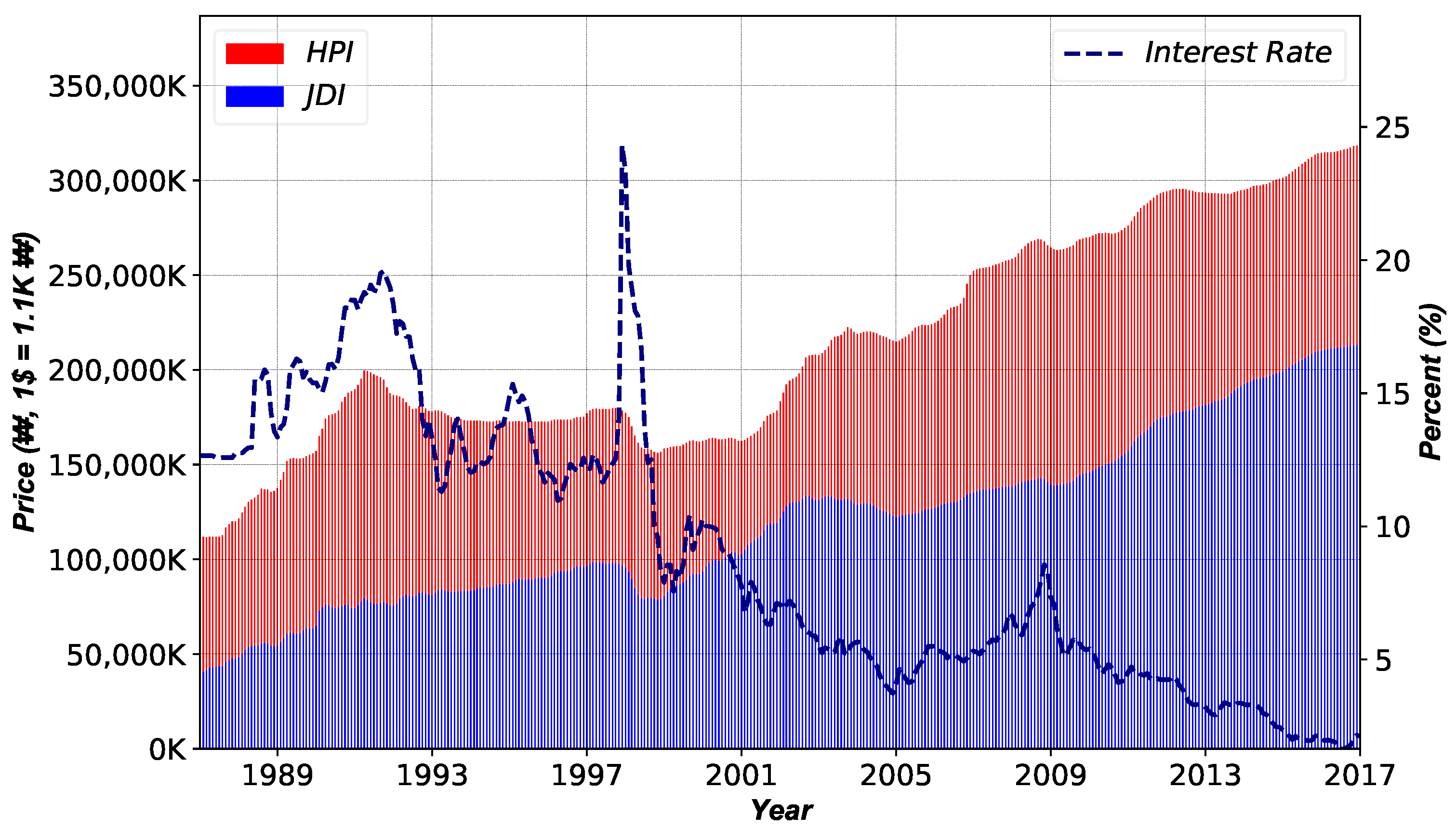
The data used in this research include the monthly prices of the House Price Index (HPI), the Jeonse Deposit Index (JDI) and the 3-year AA-corporate bond (CB3) as a standard interest rate. The data can be obtained from the Economic Statistics System (ECOS) of the Bank of Korea. The duration of the experiment was from January 1987–December 2017, which yielded 372 observations. Note that the HPI and JDI were the aggregated indices for the Korean real estate market consisting of various residential types such as detached houses, townhouses, apartments, etc. Furthermore, the CB3 is widely used in the market when a trader borrows or repays loans. Utilizing the HPI and JDI in the real options framework, we employ the CB3 as a discount factor.
Figure 1 plots the time series of the HPI, JDI and CB3. Considering the economic growth of Korea, the HPI and JDI show an up-right increasing trend with paired patterns among them. The amount of difference between the HPI and JDI changes depending on the economic conditions since the house price can be regarded as a potential future time value of housing with respect to its current value, the amount of Jeonse deposit. In contrast, the CB3, the loaning cost of buying a house, shows a decreasing trend. Interestingly, both the HPI and JDI show a sudden drop in 1998 when the bailout by the International Monetary Fund due to the foreign exchange crisis was realized. Furthermore, a rapid rise in the interest rate was observed simultaneously. In this period, speculations on house price fell over the declining levels, which incurs a decline in both the HPI and JDI. Since then, the CB3 has fallen sharply, but the appreciation of the market has not led to a rise in prices immediately. However, the JDI, which represents the current demand on residence, relatively rapidly rose, which led to the smallest spread during the experiment. Note that the spread indicates the amount of gap between the HPI and JDI. The Korean real estate market experienced an aggressive growth from the late 1980s to the early 1990s due to the rapid economic growth and government-driven urbanization on authorized land. Hence, speculations during the boom cycle were inevitable. To reduce the speculation, the Korean government deregulated the supply constraint, which suppressed the over-heated housing price [
3]. Both the HPI and JDI exhibited a huge downturn with the foreign exchange crisis in the late 1990s, but they were on a fast rise again as the economic boom cycle took place after the quick overcoming of the crisis and hosting of the 2002 World Cup. Since then, many government-driven policies failed to curb the rapid rise in house price, which still continues with the intense discussions regarding the speculation-driven bubbles in the Korean real estate market.
Table 1 summarizes the descriptive statistics of the price series of the HPI, JDI and CB3. The HPI has a mean of approximately 220 million Korean Won (KRW), roughly 200K dollars with a 1:1100 exchange rate, and a standard deviation of 59 million KRW, whereas the JDI has 120 and 47 million KRW, respectively. CB3 shows a mean of 8.7% and a standard deviation of 5.2%. The distributions of HPI, JDI and CB3 are right-skewed with their kurtosis less than the Gaussian distribution, three. Lastly, the augmented Dickey–Fuller [
71] tests show the unit roots in price series.
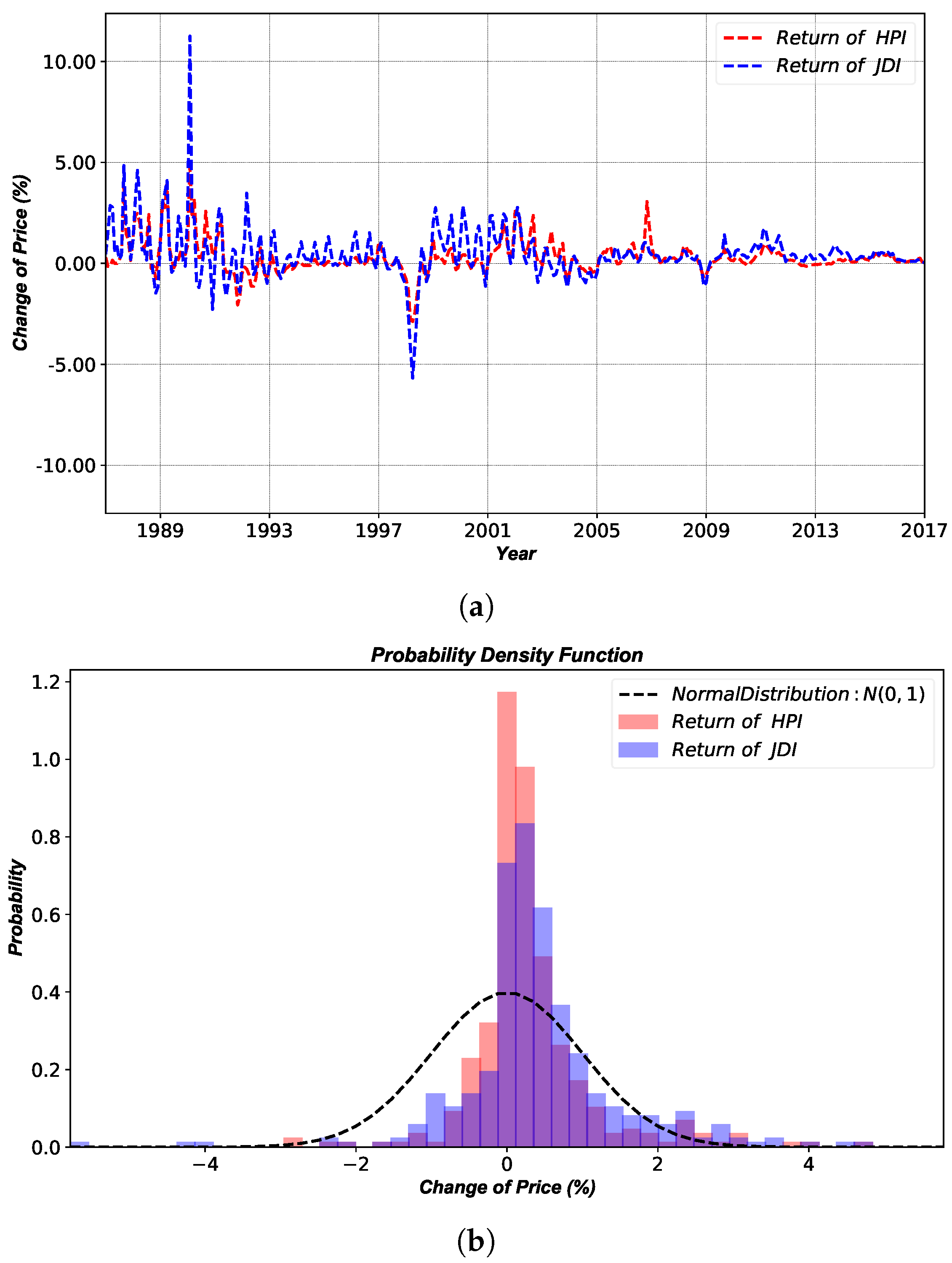
On the contrary, the return series show different descriptive statistics as illustrated in
Table 2. Although the distributions of the HPI, JDI and CB3 are right-skewed, their kurtosis is significantly greater than three. This implies that the distributions exhibit heavy-tails in comparison to the Gaussian distribution. Furthermore, the Kolmogorov–Smirnov [
72] and Jarque–Bera [
73] tests strongly reject the null hypothesis of the Gaussian assumption with 0.1% significance. The ARCH test [
74] fails to reject the assumption of no conditional heteroscedasticity in CB3. Interestingly, the ARCH test in HPI also shows a strong significance in all lags, whereas the significance becomes weakened as the lag increases in the JDI. The Ljung–Box tests [
75] on each return series show strong correlations for all indices, but the tests on the squared return series show strong correlations for the HPI and JDI only. Lastly, the ADF test shows no unit root in return series.
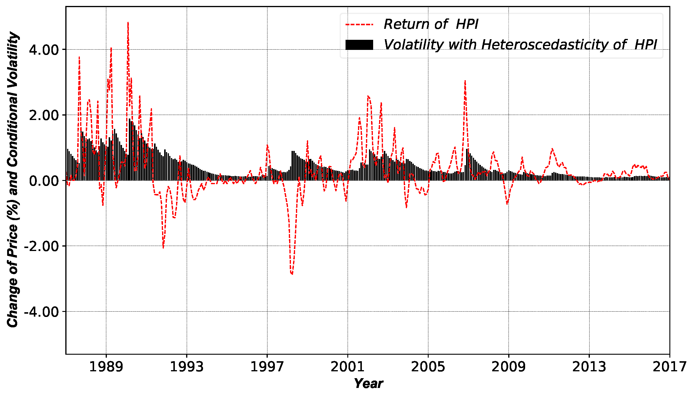
Figure 2 presents the return series of HPI and JDI with the comparison between their returns and the Gaussian distributions.
Figure 2a shows the co-movements of return series of the HPI and JDI, whereas
Figure 2b shows their heavy tails in the positive returns. The distributions of the HPI and JDI visually show less volatility than that of the stock market. However, the less the price movement, the more sensitive it is to small volatility. Furthermore, volatility clustering is observed, as the time series shows the clustered large returns [
76]. Hence, the real options framework for the HPI and JDI should include the heteroscedasticity. In conclusion, we decided to incorporate the heteroscedasticity into the binomial tree-based real options framework to measure the bubbles in the Korean real estate market using HPI and JDI.
4. Proposed Real Options Framework
4.1. Definition of the Jeonse System in Real Options
A Jeonse contract is analogous to a zero-coupon bond with a collateral. Once the contract is made, a tenant (debtor) pays the large sum of deposit to a landlord (creditor). Then, a tenant is reimbursed the deposit at maturity without paying any further fees. However, if a landlord fails to return the deposit at maturity, a Jeonse contract will pledge the house by transferring the ownership of the house to a tenant. In this context, a tenant in the Jeonse contract can be considered as possessing a long position in the call option against a landlord where the house and deposit prices are the underlying asset and strike prices, respectively. Furthermore, the landlord can be considered as possessing a long position in the put option against a tenant, simultaneously. At this point, the expiration date is when the contract is agreed upon. However, since the contract date can be canceled (early exercise) at any time under the agreement of both parties, it also can be regarded as an American option. In conclusion, a Jeonse system consists of two contracts, both before and after the contract is concluded. Therefore, the contract can be expressed as a zero-coupon bond since both parties’ payoffs are fair trade contracts that are completely hedged during the entire period.
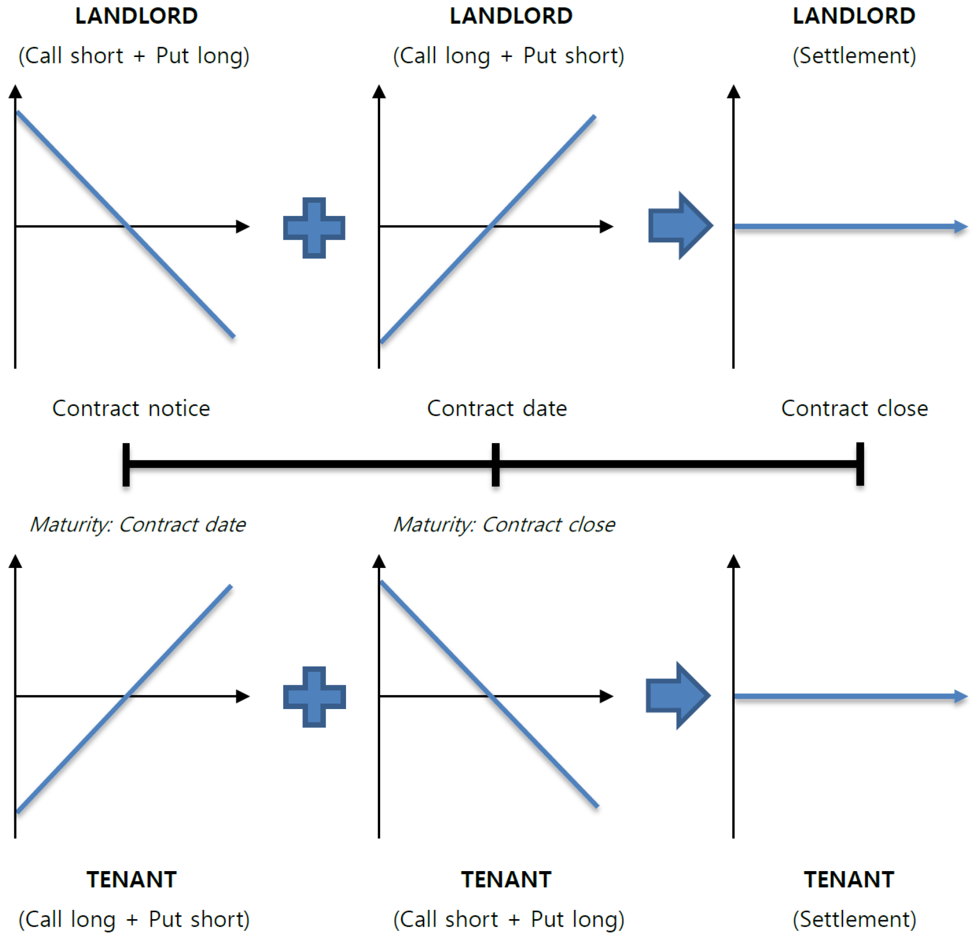
Figure 3 explains the payoffs of both parties in detail. Options trade twice for a single Jeonse contract. The first option is realized at the notification of landlord’s demand in the Jeonse contract to the market, the expiration date of which is when the Jeonse contract is signed with a tenant. The second option is realized at the date of the contract agreement, the expiration date of which is the when the Jeonse contract is matured. Note that the payoffs for both parties are exchanged for two options. This implies that the positions of a landlord and a tenant are reversed according to the movement of underlying asset prices at each time. For instance, a tenant in before the contract period is at an advantage if the price of the underlying asset rises until the contract date. On the other hand, a tenant after the contract period is favored when underlying asset price falls. A landlord has the opposite position to the tenant.
Both a landlord and a tenant face the decisions in terms of option to defer and option to abandon at the contract notice, contract date and the contract close explained in
Figure 3. Option to defer is a strategy in which an investor postpones the investment to a certain point in the future [
77,
78,
79], whereas option to abandon is a strategy to terminate the investment for the alternatives [
79,
80]. Each decision is evaluated by answering the following questionnaire and interpreting the condition of the housing market. Note that the early termination in Q3 can be realized when a landlord (tenant) sells (buys) the house or switches the counterpart in the Jeonse contract.
Q1. Before the notification of the Jeonse contract:
Actions: Trade (Option to Defer) + Jeonse (Option to Abandon)
Landlord: Should I sell (Trade) OR keep (Jeonse) the house?
Tenant: Should I buy (Trade) OR lease (Jeonse) a house for living?
Q2. From the contract notice to the contract date:
Actions: Trade (Option to Abandon/Defer) + Jeonse (Option to Abandon)
Landlord: Should I sell (Trade) the house OR agree (Jeonse) on the contract?
Tenant: Should I buy (Trade) the house OR agree (Jeonse) on the contract?
Q3. From the contract date to the contract close
Actions: Trade (Option to Abandon/Defer) + Jeonse (Option to Abandon/Defer)
Landlord: Should I terminate (Trade) the contract early OR maintain (Jeonse) the contract until the expiration?
Tenant: Should I terminate (Trade) early OR maintain (Jeonse) the contract until the expiration?
4.2. Design of the Real Options Framework
A project can be evaluated based on the options’ valuation under the future uncertainty. The main characteristics of a real option against a financial option is described as follows: (i) no expiration, (ii) no immediate exercise, (iii) difficulty in measuring the current value of the underlying asset and (iv) contributions to the supply side of the real estate market [
81]. However, as previously defined, a Jeonse contract can possess several expiration dates with an incentive for relatively immediate exercise due to fairer transaction. That is, the mutual payoffs can be canceled as compared to a trade of a house. Furthermore, the arbitrage condition, the concept of which is important in the theory of option pricing due to the law of one price [
82], can be applied to the proposed model. Since either a seller or a buyer can have a favorable position when the present value of the future prices is not equal to the current price, it implies not only the absolute gain of profit from an arbitrage opportunity, but also the loss of the opponent as opposed to the obtained profit, which suggests no difference against a financial option.
Table 3 summarizes the proposed real options framework in terms of financial option.
S and
K denote the present value and strike price of the underlying asset at the initial state, respectively;
and
represent the rate of return in profit and loss of the underlying asset, respectively; and the probabilities of the price of underlying asset in time
t as in
and
are defined as
and
, respectively, where
is satisfied. Similar to a financial option,
S and
K can be simply replaced with the HPI and JDI for the real options framework in the real estate market.
V in financial options is the value (i.e., price) of a option, whereas that in real options is the present value of future spreads in each time period. Since
V indicates the present value of the payoffs in future decisions, it also can be considered as the opportunity cost of the Jeonse contract and the time value of the house instead of choosing the purchase contract. That is, the amount of spread (i.e.,
) indicates the size of bubble by comparing with
V. Lastly, the long-term arbitrage opportunity in the financial market is limited due to the immediate transactions in short-term trades. However, the long-term arbitrage can be realized in the real estate market due to its duration of contract, which leads to a trader’s limited attention to the market information.
Regardless of a buyer of a house or a tenant in Jeonse, owning a house incurs certain costs such as tax, security, electricity, gas, water, Internet, cable, etc. Note that the costs are relatively smaller than the price of a house. Furthermore, owning a house itself does not produce a profit unless a landlord decides to rent. That is why, in general, the related studies include the indirect profits and costs in the payoffs at selling. Therefore, the house price at a trade can be seen as the present value of cash flows, the sum of future profits and the regular costs of a certain amount. In the modeling perspective, it is difficult to access the NPV problem by considering the entire future cash flows due to the discrepancy in traders’ type of housing and asset conditions. Therefore, our framework assumes the HPI as the aggregated future cash flows. The JDI, a strike price, can be regarded as the price that enables a non-house owner to immediately possess a house for a certain period of time. Specifically, a Jeonse contract sets the house as the collateral, which offsets the default risk of the deposit. Therefore, the Jeonse contract is more prompt in action than the trade by avoiding a tenant’s risk of owning a house incurred from its price change. Our proposed real options framework is derived as an American option, the exercise and liquidation of which must be possible before the expiration date. Note that the Jeonse contract has flexibility in the agreement of expiration date, early exercise and extension of the contract.
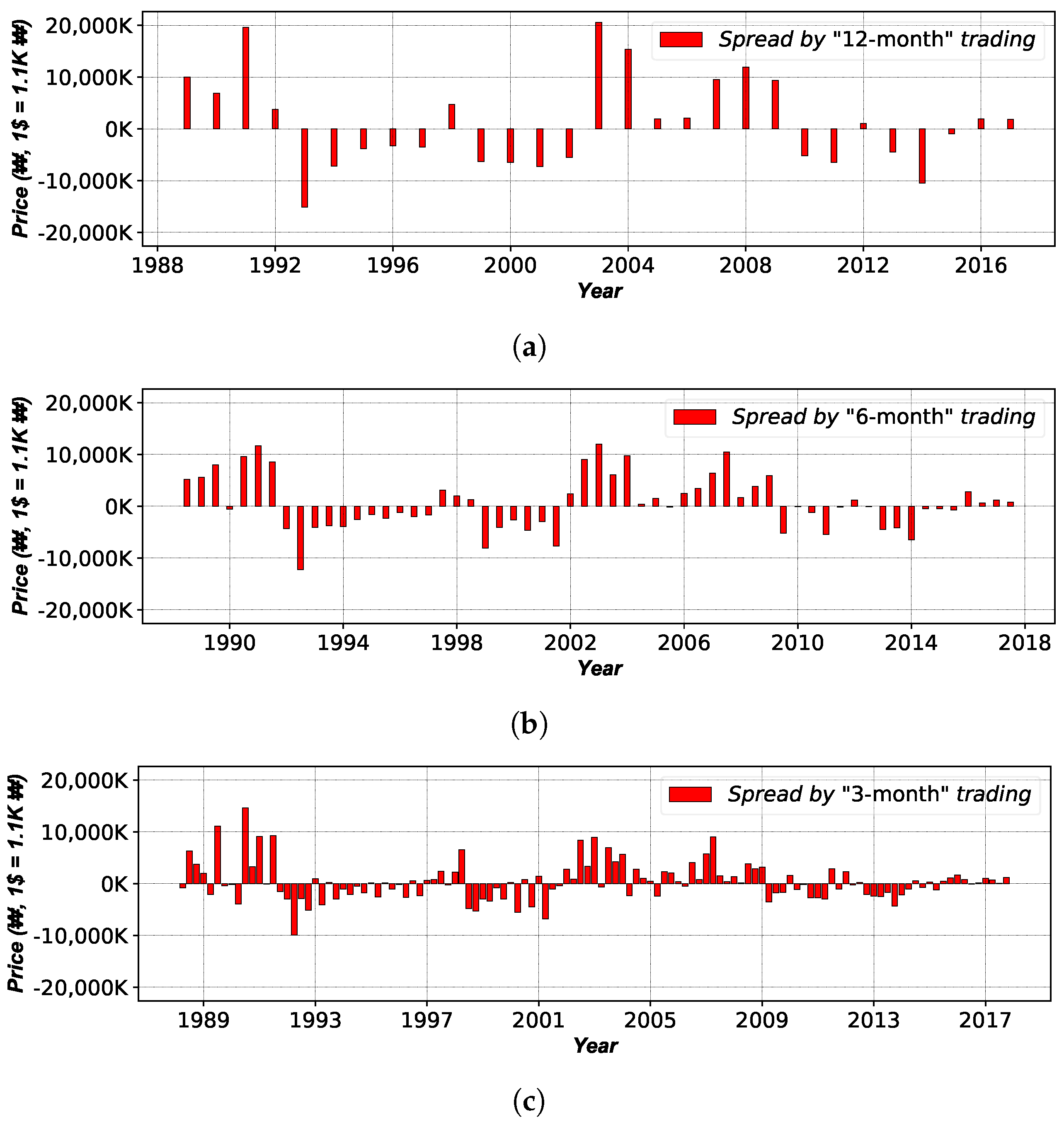
4.3. Reduced Form of Spread and Bubble
As previously explained, the values of traders’ positions are determined not only by the change of HPI, but also by that of JDI. Regardless of traders’ positions, a trade transaction depends on the HPI, whereas the Jeonse transaction depends on the JDI to settle down the investment decision. Hence, a trader simply buys (sells) a house with the expectation of the rising (falling) of its prices in the future, and likewise buys (sells) a Jeonse contract with the expectation of the rising (falling) of JDI. However, such investment without a future forecast is not an optimal decision. For example, the HPI could fail to reflect the market value of a house if the increase of JDI suddenly becomes extremely larger than that of HPI due to a rapid growth on residential demand. Such a case can occur when an alternate investment incurs higher profits. Therefore, it is problematic to decide on an investment based on one type of indicator. The advantage of utilizing the JDI lies in the consideration of pure residential price as the current value. Note that the house price itself is too volatile to be considered as the current value due to many speculative factors. Therefore, the spread should be used to measure the bubble in the real estate market by consolidating the HPI and JDI into a single valuation framework. Specifically, the spread refers to a bubble in the market given that the HPI (JDI) is the fundamental (current) value of a house. Furthermore, the utilization of spread incorporates the information regarding the house price (supply-side) and the Jeonse price (demand-side), which yields more accurate current value. In other words, the proposed real options framework in the Korean real estate market can affect not only the supply-side, but also the demand-side.
Although the decisions in questionnaires from Q1–Q3 are simply divided into three categories in
Figure 3, the decision can be made at any time during the contract in the Korean real estate market. This means that the increases of HPI in the future do not always guarantee the profits in every scenario of future time points, which becomes another reason why the spread between the HPI and JDI should be used as an indicator of bubbles in the real estate market. The spread can identify the trend of option premium and whether the house and deposit prices are rising or falling. Furthermore, the spread can be a negative value, which allows more sophisticated modeling of decision making than the series of non-negative values. We believe that the proposed framework using the spread can determine the presence of bubbles of the HPI against the JDI, the information of which eventually can be utilized to enable the arbitrage trading. In this context, the elimination of arbitrage opportunity indicates the disappearance of bubbles in the real estate market. Note that the bubbles can disappear if the market reflects the associated information through its mechanism.
Table 4 explains the direction of spread regarding the movements of HPI and JDI. Except for the case when the HPI and JDI move concurrently, there are eight cases that cause the rise and fall of spread. Specifically, between the contract notice to contract date, the increase in spread is advantageous for the landlord’s selling of the house and the tenant’s Jeonse contract, while the decline of the spread is favorable for the landlord’s Jeonse contract and the tenant buying a house. In contrast, after the contract date, the advantageous position is exchanged due to the opposite payoffs. Therefore, the expansion of bubbles in the real estate market indicates an increase in the position of house selling (decrease in demand of buying a house + increase in demand of Jeonse contract), while the shrink of the bubble indicates an increase in buying a house (increase in demand of buying a house + decrease in demand of Jeonse contract). The problem of the disagreements in investment timing between the landlord and tenant can cause difficulties in achieving the simultaneous profits of participants, which might increase the market volatility. Therefore, this study focuses on reflecting the bubble-related information, which indicates the elimination of arbitrage opportunity, into the market to assist a sustainable real estate market.
4.4. Mechanism of Volatility with Heteroscedasticity
We consider the binomial option pricing mechanism introduced in [
83] as the ground model. The ground model uses a decision tree at discrete time by assuming that the prices and returns of underlying assets follow a random walk process and a Gaussian distribution, respectively. This implies that the underlying asset follows the lognormal distribution [
84]. Furthermore, the ground model assumes the constant volatility of underlying assets over time. However, the proposed real options framework is estimated without realizing the latter’s assumption on constant volatility in order to develop a more realistic model. As a result, the proposed framework estimates the volatility of the HPI with heteroscedasticity before applying the binomial tree. That is, the proposed framework is expected to improve the numerical accuracy compared to the traditional fixed type binomial tree by setting the parameters reflecting the trend and volatility. Furthermore, we incorporate the results of [
85] where the supply conditions are related to the movement of volatility of price (speculation), whereas the demand conditions contribute to run-up and collapse in the real estate markets. Specifically, we employ the Jeonse price and estimated volatility with heteroscedasticity to represent the demand condition and the information of supply condition, respectively. For this purpose, we derive a mathematical model to design the real options framework as follows. As shown in
Figure 2, the real estate market is less volatile than other financial assets. However, it is hard to state that the volatility is constant at all times given that the real estate market is highly sensitive to the regime shifts in related policy. Hence, we upgrade the ground model by consolidating the volatility with heteroscedasticity to evaluate a more realistic value of the real options. The house price,
, depends on time,
t, by following the geometric Brownian motion such that,
Since the price series are not stationary as described in
Table 1, we incorporate the return series for modeling. Specifically, the house price can be modeled based on the geometric Brownian motion,
where
is the standard Brownian motion in the risk-neutral Q-measure. Considering Ito’s lemma with
yields,
with the following conditions,
Furthermore, since the multi-period binomial tree satisfies
, the following equations can be established under the risk-neutral condition.
Equations (
6) and (7) are approximately equivalent to the following equations.
where
,
and
are estimated based on the probability equations derived from
and
and the trend of the stochastic process in
and
.
In the case of the underlying assets of financial products, the past data are analyzed to predict the probability of rise and fall in the near future. However, the interpretation of the probability of rise and fall in the real estate market is slightly different. Most traders in the real estate market consider a house as a necessity for their residence. Furthermore, it is more difficult to predict the probability of future price movement since a transaction in the real estate market is not frequent in comparison to that in the financial market. The estimation of probability is even unrealistic since the price of a house is more dependent on the government policy than its endogenous value. Hence, in this research, we suggest setting
. It is an expression stating that the prediction of probability is meaningless. In this condition, we can derive the equations for
and
that satisfy the following equations.
Our approach cannot reflect the trend with
and
like other traditional binomial trees in the ground model since
. Instead, we propose the utilization of
and
to incorporate the trend. The realization of the binomial tree with the trend in the proposed real options framework can be accomplished by implementing
,
and
in a pre-estimated heteroscedasticity at each time point as follows.
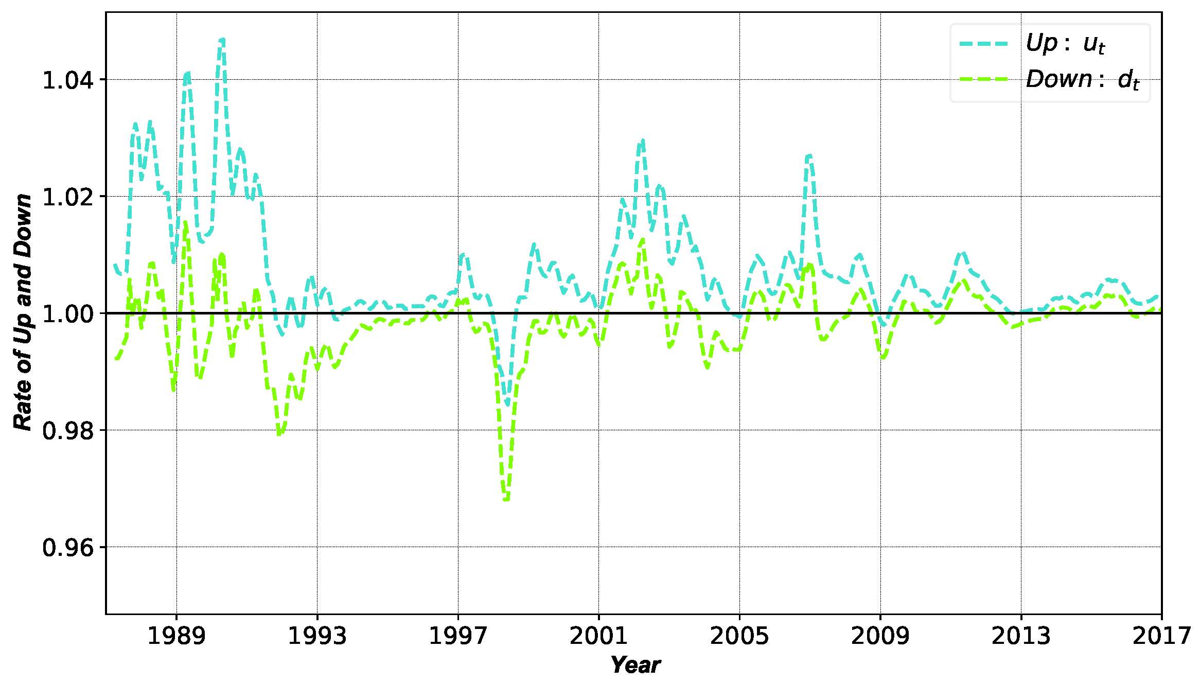
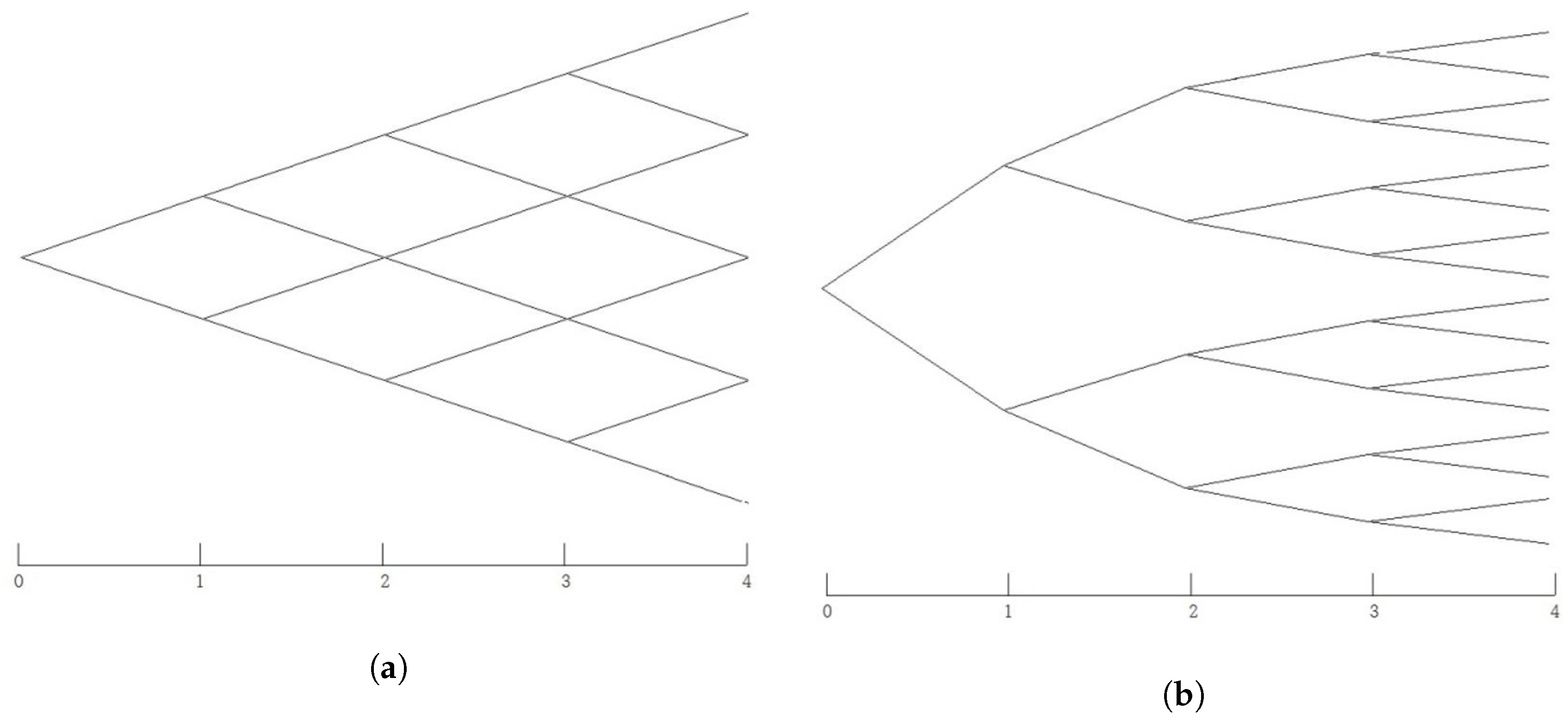
In the case of using , and volatility with heteroscedasticity, the shape of the binomial tree is different from the conventional one. In the conventional case, , and are equal to , and , respectively, after two periods where the joint nodes exist in each time period. However, there are no joint nodes when the volatility with heteroscedasticity is used. That is, the structure of the binomial tree is determined by and rather than and .
Figure 4 visualizes the difference between the conventional and proposed binomial trees. In the conventional tree model, the probability of each node at maturity represents the form of a Gaussian distribution, the value of which becomes larger toward the middle. However, the proposed binomial tree derives more sophisticated future scenarios with many possible cases since it assumes the same probability for each node. More detailed mathematical background regarding the nodes and heteroscedasticity is described in [
86]. Furthermore, the direction of the proposed binomial tree is different from that of the conventional one. The conventional model use the tree structure that stretches up and down after removing the trend. However, the proposed binomial tree allows the trend included in the equations of
and
with fixed probability. Therefore,
is larger than
when the price rises, whereas
is smaller than
when the price falls. Furthermore, both
and
can have a value greater than one or less than one by reflecting the trend of HPI.
The important feature of the proposed real options framework is considering the volatility with heteroscedasticity. The implementation of heteroscedasticity is as follows. At first, the volatility with heteroscedasticity is estimated based on the time series estimates of and . If there is sufficient data, the volatility () is set to be the variance over the past period or the mean of variances over all periods if the assumption of equal variance is valid. However, in this study, we estimate the volatility with heteroscedasticity using a time series of returns. Secondly, we apply the proposed tree approach with the specified at each time point. In our model, one period, , is equal to one month, and at each time point is set to be the mean of the past returns for the number of lost data in the volatility estimation. Lastly, we determine at each time point to reflect the heteroscedasticity.
6. Conclusions
The U.S. sub-prime mortgage crisis began with the collapse of bubbles in its real estate market. The riskiness of the burst of bubbles is then presented by triggering an outbreak of global financial crisis. In this context, we attempt to measure and manage the bubbles as a way to support the sustainability of the Korean real estate market. Therefore, the main task of this study is to develop a mathematical framework to measure the bubble in the market by consolidating the unique system called the Jeonse and the volatility with heteroscedasticity.
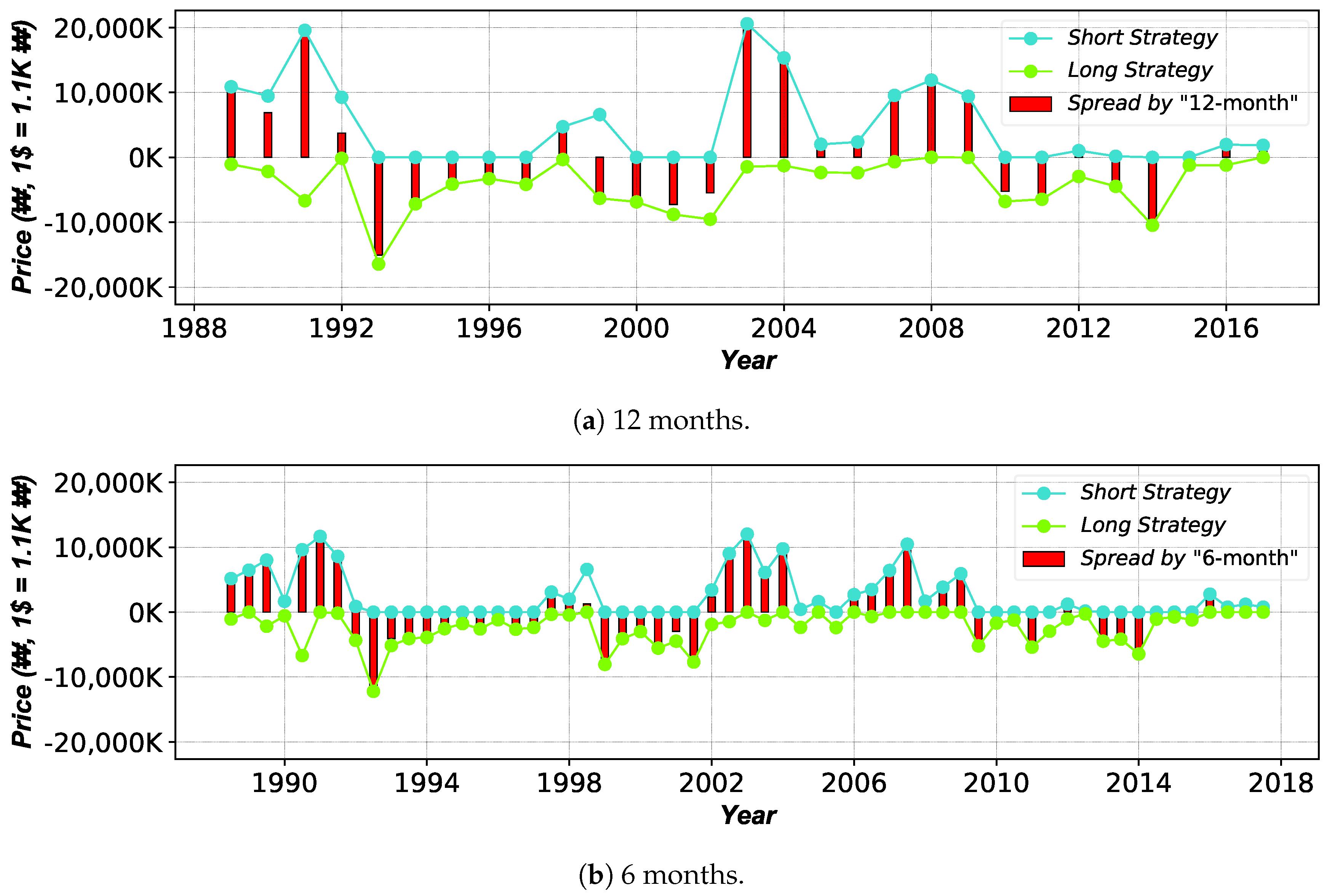
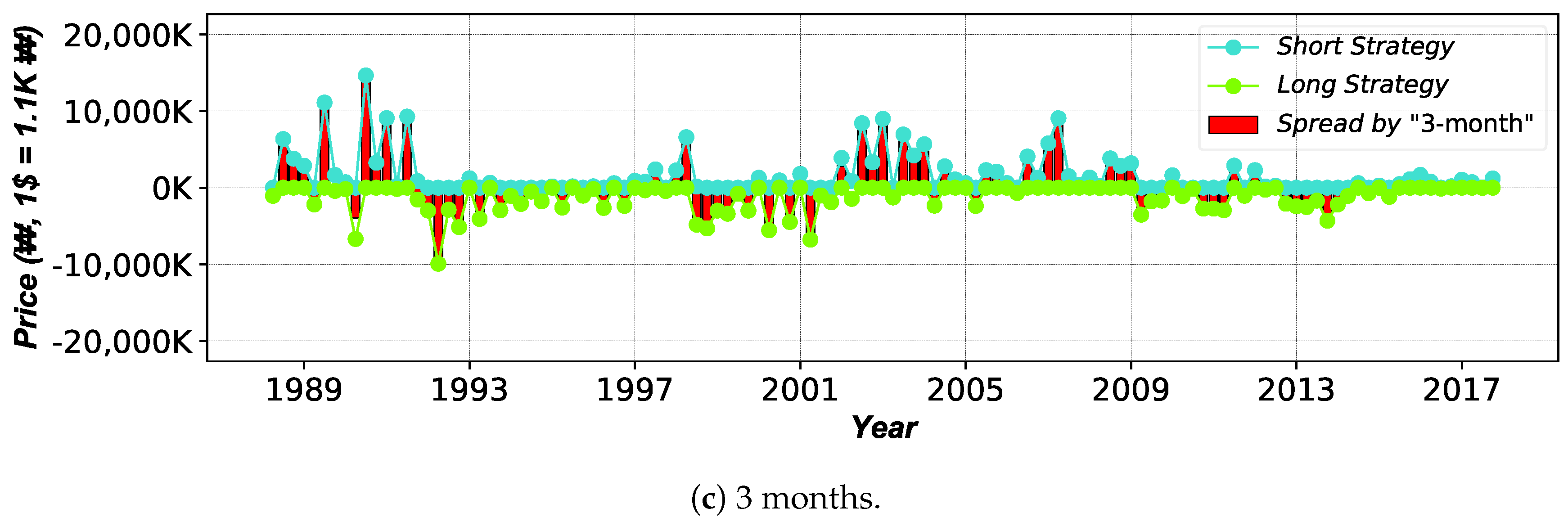
Our paper is novel in that, to our best knowledge, this is the first attempt to measure the bubbles in the Korean real estate market in the real options framework. Based on the proposed model, we discover some interesting findings as follows. At first, by analyzing its system, we discover that the Korean real estate market can be interpreted in terms of financial options. Especially, the Jeonse deposit can be utilized in order to evaluate the size of bubbles in the real estate market. Secondly, we describe that the Jeonse system is freed from the default risk, which can avoid the loss of investment, as well as the risk of uncertainty that might arise from possessing a house. Furthermore, we explain that the Jeonse system has the characteristic of an American option with more flexible liquidation. Thirdly, utilizing the HPI and JDI, we propose the binomial tree with heteroscedasticity to set the investment decision in short and long positions. The proposed framework provides the size of bubbles and the existence of arbitrage opportunity in the market based on the present value of future spreads. Note that the appropriate investment timing and decision can be suggested by the measured bubbles.
Furthermore, we discover that traders are able to hedge the risks of their positions through early exercise when the information regarding the bubble in the real estate market is provided. The trading results prove that the early exercise eventually leads to the reduction of bubbles by eliminating the arbitrage opportunities, which also suggests that the proposed model successfully measures the bubble. Such a phenomenon indicates that the opportunity for a bubble to exist in the market disappears. As illustrated in [
69], the exercise of options decreases the volatility of the underlying asset (i.e., house price) with quick adjustment on new information. That is, the trading strategies based on the proposed real options framework contribute to the stability of the real estate market by reflecting the bubble-related information through a market mechanism. We also believe that the findings of our paper can assist the careful decisions among traders in the real estate market, construction firms and related policy-makers. Although the Korean real estate market has the characteristic of an American option, traders often abandon early exercise by maintaining the contract until maturity due to the lack of information and market uncertainty. Hence, the sharing of bubble-related information is expected to promote the price adjustments led by individual traders. Furthermore, the construction firms can utilize the proposed framework in measuring the reasonable price of a house as a basic supplier of housing, whereas the related policy-makers can use our findings to monitor the bubble of the market and to avoid the excess supply of housing.
The drawbacks of this paper that should be addressed in a future study are as follows. At first, there is a difficulty in applying the model to other countries due to the absence of the Jeonse system. That is, the merits of the findings solely remain in the case of Korea. However, the implications of this paper can be helpful in considering the Jeonse system as a new method of housing in other countries. The simple application is also possible to some extent by using the conversion of monthly rent. Note that the amount of Jeonse deposit can be informally converted from the amount of monthly rent as described in
Section 1. Furthermore, this study only provides the macro-economic perspective of the bubble in the Korean real estate market since we only use the nation-wide indices, HPI and JDI. The scope of the current indices is too broad to be used for an investment in individual property given that the price of trade and Jeonse varies depending on the region and type of housing. Hence, for further research, we are planning to co-work with the online real estate brokers to test the suitability of the proposed framework by utilizing the daily or weekly prices of individual property in different regions.


