Evolving Temporal–Spatial Trends, Spatial Association, and Influencing Factors of Carbon Emissions in Mainland China: Empirical Analysis Based on Provincial Panel Data from 2006 to 2015

Abstract

Based on provincial panel data from 2005 to 2016, this paper analyzes evolving temporal–spatial trends, spatial correlation and influencing factors of carbon emissions in China. The results show that there is a great heterogeneity in the evolving temporal–spatial trends of carbon emissions among provinces and regions in China, with the heterogeneity in eastern provinces most obvious. At the same time, there exists significant spatial correlation and agglomeration of carbon emissions in 30 provinces. It is found that the distribution characteristics of carbon emissions are affected by various economic and social factors based on the extended STIRPAT (Stochastic Impacts by Regression on Population, Affluence, and Technology) model. Population pressure, affluence, energy intensity, industrial structure, urbanization level and investment in fixed assets can significantly promote the increase of carbon emissions. The technological level and government environmental supervision have significant inhibitory effects on carbon emissions, but foreign direct investment (FDI) has no significant impact. Therefore, it is necessary to strengthen environmental supervision and upgrade technology level to promote carbon emission reduction.

Highlights

(1)

Analysis of the temporal–spatial trends and spatial correlation of CO₂ in China’s 30 provinces.

(2)

Research on the influencing factors based on the extended STIRPAT model.

(3)

There exists great heterogeneity and significant spatial correlation of CO₂.

(4)

It is necessary to strengthen environmental regulation and improve technological level to promote carbon emission reduction.

1. Introduction

The immunity period for developing countries under the Kyoto Protocol ended in 2012. The post-Kyoto negotiations should pay a lot of attention to substantial obligations for developing countries. As the largest developing country, China will face increasing pressure in emission reduction. In tandem with rapid development of the economy, massive energy consumption has made China the country with the world’s largest overall carbon emissions and it has played an important role in global carbon emission reduction works. On 14 November 2016, the Global Carbon Project (GCP) released the “Global carbon budget 2016”, which shows that global carbon emissions are already getting rid of the rapid growth trend of the last decade in a dramatic and unprecedented way, and the reduction of using coal in China is the main reason. China’s carbon emissions reached 10.4 billion tons in 2015, accounting for 29 percent of the global total amount, and it increased by an average of 5.3 percent every year from 2005 to 2014. However, it decreased by 0.7 percent in 2015 and kept a continuous reduction trend in 2016 [1]. On 13 November 2017, the GCP released the “Global carbon budget report 2017” at The United Nations Climate Change Conference in Bonn. The report points out that in 2017, the world’s fossil fuels and industrial carbon dioxide emissions are expected to grow by 2 percent, which is the first increase in global carbon emissions since falling for three years from 2014. China’s carbon emissions are expected to grow by about 3.5 percent in 2017, whose total amount will exceed the sum of the 28 countries of the United States and the European Union. In addition, carbon dioxide emissions per capita and per unit of GDP will also be significantly higher than the world average [2]. A variety of factors indicate that global carbon emissions will continue to increase in the future, so energy saving and emission reduction in China is facing more serious challenges.

In fact, since entering the 21st century, the Chinese government has paid great attention to environmental governance and intensified its efforts to save energy and reduce emissions. The period 2006–2010 and 2011–2015 are respectively the implementation period of the “11th Five-Year Plan” and the “12th Five-Year Plan” of China. At the Copenhagen United Nations Climate Change Conference (2009) and the Paris Conference (2015), China committed to “cut the CO₂ emissions per unit of GDP by 40–50% by year 2020 from the year 2005 level” and “carbon dioxide emissions per unit of GDP will fall by 60–65% by 2030 from 2005 level.” From 2010 to 2015, China’s environmental protection polices received unprecedented attention, and total investment in environmental governance as a share of GDP has increased, and the energy consumption per unit of GDP is also declining. Previous studies have shown that the increase or decrease of carbon emissions is directly or indirectly affected by various economic and social factors, including the population size, economic development, the urbanization process, industrial structure, the energy consumption, the foreign direct investment and so on [3,4,5]. However, China is a centralization country that has a long history of the unitary system; at the same time, it is in a period of social transition. Compared with developed countries, the of government control often play a more prominent role in energy saving and emission reduction work; moreover, the environmental regulation also mainly takes the administrative order as its mean [6]. Therefore, in this context, the influencing factors of China’s carbon emissions will not be the same as other countries, which need to be further studied.

It is worth noting that China is a vast country with many provinces, and has some of the largest gaps in natural geography, population resources, economic and social development in the world. The problems faced by numerous provinces and regions in the process of energy saving and emission reduction are also very different. However, previous studies have shown that the environmental quality, especially air quality, has a great spatial correlation. Due to the influences of wind and turbulent motion in the atmosphere, pollution source can spread rapidly when emitted into the atmosphere [7]. In addition to natural conditions, the economic and social factors in different regions also connect and influence each other. For example, the level of economic development in neighboring regions also has certain similarities, leading to the regional relevance of energy consumption and carbon emissions [8]. Furthermore, technologies which are related to environmental protection have “spatial spillover” effects [9]; even the policies on energy saving and emission reduction of regional governments have certain relevance and “positive externality”. If a certain area implements very strict environmental control measures, it can improve not only the local environmental quality, but also the environmental quality of the neighboring regions, thus reducing carbon emissions from the adjacent areas. Therefore, carbon emissions in a region will not only be affected by the surrounding areas, but also affect carbon emissions of surrounding areas. With this background, it seems to be necessary and meaningful to measure carbon emissions in various regions of China and analyze the regional differences and spatial correlations as well as the influencing factors. Therefore, this paper will use the panel data from 2006 to 2015 to analyze the evolution trend and spatial correlation of carbon emissions in various provinces of China and studying the influencing factors on this basis. The studies in this paper cannot only grasp the evolving temporal–spatial trends of carbon emissions in different regions of China, but also provide some suggestions for energy saving and emission reduction work in the future.

2. Literature Review

2.1. Calculation of Carbon Emissions and Its Spatial Correlation

The Intergovernmental Panel on Climate Change (IPCC) put forward that in addition to nature itself, the increase of greenhouse gases mainly derives from the combustion of fossil fuels by human beings. At the same time, it also proposed a method to measure and calculate carbon emissions based on the number of fuel combustion factors [10]. Many scholars have used the method proposed by the IPCC to do research estimating carbon dioxide emissions. Based on energy statistics, ref. [11] estimated the global carbon dioxide emissions in 1971–2004. Ref. [12] estimated the amount of carbon emissions from developed, developing and less developed countries, finding that in 2004, the developing and less developed countries, which account for approximately 80 percent of the world’s population, only accounted for 41% of the world’s carbon emissions. Based on the IPCC method, refs. [13,14] estimated carbon emissions in the UK and South Korea respectively, and considered that the growth of fossil fuels, such as petroleum, was the main cause of carbon dioxide growth. Ref. [15] estimated carbon emissions of 30 provincial capitals in China in 1990, 2000 and 2010 using the carbon emissions coefficient and the corresponding energy consumption. However, the time points are discontinuous, so they cannot analyze temporal–spatial trends. Because of the limited sources of carbon emission data in China and the lack of direct monitoring data on carbon dioxide emissions in various provinces, this paper will estimate the total amount of carbon emissions based on the major energy consumption of each province in 2006–2015 and analyze its temporal–spatial trends.

At present, most of the existing literature on the total amount of carbon emissions of some provinces in China only stays at the level of descriptive analysis, and there is scant literature that deeply explores the regional differences as well as their temporal and spatial variation characteristics. Furthermore, the amount of literature that makes systematic and comprehensive studies of its influencing factors is even smaller. Spatial interaction theory shows that the observed values of pollutant concentrations in different regions are not independent of each other, and there is obvious interaction between them. Ref. [16] found that the distribution of carbon emissions in China is very uneven, which is shown by the fact that about 35 cities with 18% of the total population contribute 40% of carbon emissions. This shows that the distribution of total carbon emissions in major cities in China is very different, and there are agglomeration trends in some provinces. Therefore, the spatial pattern of carbon emissions in various provinces also needs to be studied. Ref. [17] analyzed the spatio-temporal dynamic evolution of carbon emissions in China from 1985 to 2008. The result shows that the per capita carbon emissions in northern and western regions of China are higher than those in the eastern regions, whose economy is developed. Ref. [18] measured the spatial pattern of per capita carbon emissions from 1995 to 2011 by using the spatial auto-regression model. The research shows that although the spatial auto-regression of per capita carbon emissions in China is decreasing year by year, the total amount of per capita carbon emissions shows an increasing trend year by year. In the last five years, there has been scant literature that measures and calculates the total amount of carbon emissions in China’s provinces and the spatial and temporal trends as well as their spatial correlation, because the administrative region is not only the implementation area of carbon emission reduction, but also the main distribution of carbon emission reduction. To achieve the goal of carbon emission reduction, it is necessary to analyze the spatial and temporal patterns of carbon emissions in different regions and provinces, to formulate and implement different policies and measures for carbon emission reduction, which are in accordance with the evolving temporal–spatial trends of different regions.

2.2. Analysis on the Influencing Factors of Carbon Emissions

The existing literature mainly studies the influencing factors of carbon emissions around three levels: (1) Research on the influencing factors of carbon emissions at the national level: for example, ref. [19] studied the relationship between carbon emissions, energy consumption and economic structure in many sub-Saharan African countries by using the Laspeyres model. Ref. [20] found the main factors that affect carbon emissions in China and India are the per capita income and trade openness. Refs. [21,22,23] researched the relationship among carbon emissions, energy consumption and economic growth in Russia, Brazil, and the Middle East countries by analyzing panel data, which shows that economic growth and increased energy consumption have significantly stimulated the increase of carbon emissions. Ref. [24] found that both the per capita GDP, industrial structure, population, urbanization level and technology level can affect carbon emissions in China based on the Path-STIRPAT model. Ref. [25] using panel data empirically analyzed the effects of urbanization, energy consumption and per capita GDP on CO₂ emissions in BRICS countries. The results show that urbanization can promote the increase of carbon emissions in all countries, but the impact of per capita GDP and energy consumption on carbon emissions is different in different countries. Based on the relevant data of 36 developing countries from 1980 to 2000, ref. [26] analyzed the effect of economic growth, energy consumption, trade openness and urbanization on carbon emissions in Malaysia by using the STIRPAT model. The results show that economic development is conducive to the increase of carbon emissions, but there is a U-shaped relationship between urbanization and CO₂ emissions. (2) Research on the influencing factors of carbon emissions at the regional (or urban) level: ref. [27] studied the influence made by urbanization level, the economic level, the proportion of the tertiary industry and energy consumption on carbon emissions in Beijing. It turns out that the level of urbanization is the main driving factor of CO₂ emissions, and the tertiary industry is the main restraining factor. Ref. [28] studied the influence caused by urbanization, industrialization, and economic development level on carbon emissions in Tianjin by using the STIRPAT model. Ref. [29] analyzed the influencing factors of carbon emissions in Xinjiang by using the extended STIRPAT model. They concluded that the population scale, economic growth, investment in fixed assets and other factors have different effects on carbon emissions in different periods. Ref. [30] found that the main factors influencing CO₂ emissions such as population size, industrial structure, urbanization, and technology level have different impacts in different regions by using the STIRPAT model. (3) Research on the influencing factors of carbon emissions at the industrial level: ref. [31] found that the key influencing factors of CO₂ emission of power generation industry in China are population, per capita GDP, standard coal consumption and thermal power specific gravity by using the STIRPAT model. Ref. [32] adopts the Log Mean Divisia Index (LMDI) method to explore the impact induced by labor productivity, energy intensity, and industry scale on carbon dioxide emissions in China’s heavy industry. Ref. [33] studied the relationship between energy consumption, economic growth, and carbon emissions of industrial sectors in Canada based on cointegration analysis and the Granger causality test. After analyzing the previous literature, it is found that many methods are used by the scholars to study the influencing factors of carbon emissions, including (1) constructing the decomposition model of carbon emissions, such as the Laspeyres model, the LMDI model and so on; (2) constructing the traditional panel data regression model; (3) using the method of cointegration analysis and Granger causality test; (4) constructing the KAYA identity and IPAT model etc. At national and regional levels, the vast majority of scholars choose to use the STIRPAT model to make empirical analysis on the factors that affect carbon emissions, including the economic growth, the degree of affluence, the level of urbanization, the population size, the energy structure, the industrial structure, and other economic and social factors. However, at preset, most of the literature uses panel data to analyze the effect of different factors on carbon emissions. Moreover, previous research models usually assume that carbon emissions are independent of each other. In fact, environmental factors, especially air quality, must have a certain spatial correlation. This leads to the existence of certain deviation in the research conclusions of previous literature. Therefore, introducing the spatial panel model can accurately grasp the spatial impact of various factors on carbon emissions, and explore the direction and degree of influence about different factors from a spatial perspective.

To sum up, there is scant literature that analyzes the spatial distribution condition, regional characteristics, and their influencing factors of carbon emissions in various regions of China. However, accurate knowledge of the spatial and temporal distribution of carbon emissions and its cluster status is more conducive to targeted carbon emission reduction in different regions. Therefore, it is necessary to analyze the dynamic trends of spatial and temporal patterns of carbon emissions in different scales and regions, at the same time, using the spatial panel model to quantify the main influencing factors of carbon emissions in different scales and different regions and provide the decision-making basis for every province in China, thus helping them formulate scientific and reasonable policy for reducing carbon emissions. On the basis of constructing and extending the STIRPAT model, this paper makes an empirical analysis based on the panel data of 30 provinces in China from 2006 to 2015 to study the regional differences of carbon emissions and their influencing factors in depth by analyzing the spatial correlation and constructing spatial panel model, so as to clarify the situation of each province and provide guidance for the future work of energy conservation and emission reduction in China.

3. Research Design

3.1. Calculating Formula for Carbon Emissions

This paper selects eight main kinds of energy sources including coal, coke, crude oil, gasoline, kerosene, diesel oil, fuel oil, natural gas. Based on the method proposed by the IPCC, we can calculate carbon emissions generated by each kind of energy consumption and then obtain the total amount of carbon emissions after addition. The calculating formula is shown in formula (1), in which the $E_i$ means the amount of consumption of the $i$ type of energy, $i=1,2,\dots ,8$; ${\eta }_i$ is the carbon emissions coefficient of the $i$ type of energy. In this paper, data about 8 kinds of energy consumption of 30 provinces in China from 2006 to 2015 are from the China Energy Statistical Yearbook (2007–2016), according to the IPCC Guidelines for National Greenhouse Gas Inventories and referring to previous relevant literature [34], the carbon emissions coefficient for various energy sources can be obtained in

Table 1. Carbon emissions coefficient of various fossil fuels.

Type of Energy	Coefficient of Carbon Emissions (104 t/104 t)	Type of Energy	Coefficient of Carbon Emissions (104 t/104 t)/(104 t/108 m3)
Coal	0.775	Kerosene	0.574
Coke	0.855	Diesel oil	0.591
Crude oil	0.586	Fuel oil	0.618
Gasoline	0.553	Natural gas	0.448

.

$$C={\displaystyle \sum E_i}\times {\eta }_i$$

(1)

3.2. Spatial Autocorrelation Analysis

Making the spatial autocorrelation analysis can reveal the correlation of various elements in the process of spatial evolution. This paper analyzes the autocorrelation of global space and autocorrelation of local space of carbon emissions from 30 provinces in China to understand their spatial distribution characteristics. The global Moran’s I index can reflect the similarity of carbon emissions in adjacent regions, which has the following equation:

$$MoranI=\frac{n{\displaystyle \sum _{i=1}^n{\displaystyle \sum _{j=1}^n{w}_{ij}\left(x_i-\overline{x}\right)\left(x_j-\overline{x}\right)}}}{{\displaystyle \sum _{i=1}^n{\displaystyle \sum _{j=1}^n{w}_{ij}{\displaystyle \sum _{i=1}^n{(x_i-\overline{x})}^2}}}}=\frac{{\displaystyle \sum _{i=1}^n{\displaystyle \sum _{j=1}^n{w}_{ij}\left(x_i-\overline{x}\right)\left(x_j-\overline{x}\right)}}}{S^2{\displaystyle \sum _{i=1}^n{\displaystyle \sum _{j=1}^n{w}_{ij}}}}$$

(2)

$S^2=\frac{1}{n}{\displaystyle \sum _{i=1}^n{\left(x_i-\overline{x}\right)}^2}$, $\overline{x}=\frac{1}{n}{\displaystyle \sum _{i=1}^n{x}_i}$, n represents the number of geographical units, $x_i$ represents the observed values of carbon emissions on each spatial unit, $w_{ij}$ is the element of spatial weight matrix. When constructing spatial weight matrix, if the two regions are adjacent, then the $w_{ij}$ value is 1, otherwise the $w_{ij}$ value is 0. In this paper, we use the nearest K-point relation method to determine the spatial weight, taking K value as 4, to ensure that each province has at least one adjacent region [35]. When using the Geoda software to construct spatial weight matrix, we can calculate the index of Moran’s I, whose value range is [−1, 1]. When Moran’s I < 0, it means that there is negative spatial autocorrelation of the carbon emissions values in adjacent regions. When the Moran’s I > 0, it means that the positive spatial autocorrelation of carbon emissions existed. The absolute value of Moran’s I indicates the magnitude of spatial autocorrelation, the greater the absolute value is, the higher the degree of spatial correlation is. Moran’s I = 0 indicates that there is no spatial correlation in carbon emissions. In this paper, the significance level of global Moran’s I index is measured by standardized Z-value through the following formula;

$$\mathrm{Z}(\mathrm{M}\mathrm{o}\mathrm{r}\mathrm{a}\mathrm{n}’\mathrm{s}\mathrm{I})=\frac{\mathrm{M}\mathrm{o}\mathrm{r}\mathrm{a}\mathrm{n}’\mathrm{s}\mathrm{I}-\mathrm{E}(\mathrm{M}\mathrm{o}\mathrm{r}\mathrm{a}\mathrm{n}’\mathrm{s}\mathrm{I})}{\sqrt{\mathrm{V}\mathrm{A}\mathrm{R}(\mathrm{M}\mathrm{o}\mathrm{r}\mathrm{a}\mathrm{n}’\mathrm{s}\mathrm{I})}}$$

(3)

The expected value and variance of Moran’s I index are respectively represented by the E (I) and VAR (I). Because the critical value of normal distribution function at 0.05 level is 1.96, if the value is greater than 1.96, then the spatial autocorrelation is significant.

The local indicator of spatial association (LISA) is used to measure the spatial aggregation degree of carbon emissions between each province and its surrounding areas [36], and the Moran’s I scatter plot can be drawn by software, which has the following equation:

$$I_i=\frac{(x_i-\overline{x})}{S^2}{\displaystyle \sum _j{W}_{ij}(x_j-\overline{x})}$$

(4)

When the value of $I_i$ is a positive number, it indicates that the value of carbon emissions in the province is similar to that of the adjacent areas (“high-high” or “low-low”); if the value of $I_i$ is the negative number, it represents the attribute value of this space unit is not similar to the adjacent areas (“high-low” or “low-high”). The Moran’s I scatter plot is divided into four quadrants, which corresponding to the four kinds of forms in local spatial relations between the spatial units and adjacent units respectively. The first quadrant is “high-high” quadrant, indicating that the adjacent provinces are high-carbon-emitting areas, the second quadrant is “low-high” quadrant, indicating that the low-carbon-emitting provinces are surrounded by high-carbon-emitting provinces, and the third quadrant is “low-low” quadrant, indicating that the surrounding areas are low-carbon-emitting provinces, the fourth quadrant is “high-low” quadrant, indicating that high-carbon-emitting provinces are surrounded by low-carbon-emitting provinces.

3.3. STIRPAT Model and Spatial Econometric Model

3.3.1. STIRPAT Model and Variable Measurement

The IPAT identity constructed by [37] indicates that population increase is an important factor leading to the increase of environmental pressure, and it is generally accepted by scholars. Ref. [38] have constructed a random regression model based on IPAT identity, that is, the STIRPAT model, which has the following form:

$$I_{it}=a{P}_{it}{}^b{A}_{it}{}^c{T}_{it}{}^d{\mathsf{\epsilon }}_{it}$$

(5)

where I represents environmental pressure (Impact), P means population number (Population), A means affluence degree (Affluence), T is the technology, i and t represent the province and year respectively. a represents the coefficient. b, c, and d are the exponents of population, affluence, and technology, and $\epsilon$ is the error term. In this paper, the total amount of carbon emissions (C) is used to express the environmental pressure in various provinces. Based on STIRPAT model, the model is expanded and improved by adding six influencing factors such as environmental regulation (ER), energy consumption intensity (EC), industrial level (IL), urbanization level (UL), foreign direct investment (FDI) and investment in fixed assets (IFA).

$$C_{it}=a{P}_{it}{}^b{A}_{it}{}^c{T}_{it}{}^{d}E{R}_{it}{}^{\mathrm{e}}E{C}_{it}{}^{f}I{L}_{it}{}^{g}U{L}_{it}{}^{h}FD{I}_{it}{}^{i}IF{A}_{it}{}^j{\mathsf{\epsilon }}_{it}$$

(6)

When the logarithmization treatment is made on both sides of Equation (6), the model can be extended as follows:

$$\begin{array}{l}\ln C_{it}={\beta }_0+{\beta }_1\ln P_{it}+{\beta }_2\ln A_{it}+{\beta }_3\ln T_{it}+{\beta }_4\ln E{R}_{it}+{\beta }_5\ln E{C}_{it}\\ +{\beta }_6\ln I{L}_{it}+{\beta }_7\ln U{L}_{it}+{\beta }_8\ln FD{I}_{it}+{\beta }_9\ln IF{A}_{it}+\ln {\epsilon }_{it}\end{array}$$

(7)

In this paper, the degree of affluence is measured by per capita GDP (pgdp) of each province; and the technology is measured by number of patent license of each province, ER is measured by the number investment in environmental governance, EC is measured by the energy consumption per unit of GDP, IL is measured by the proportion of the second industry in GDP, UL is measured by the proportion of urban population to the total population; FDI and IFA is measured by foreign direct investment and fixed asset investment respectively. The above data use the original data in the statistical yearbook, including the China Statistical Yearbook (2007–2016), China Energy Statistical Yearbook (2007–2016) and so on. Among them, $\epsilon$ is the random error term, ${\beta }_0$ is the constant term, ${\beta }_1$, ${\beta }_2$ …… ${\beta }_9$ are the coefficients of elasticity, which represent the change of carbon emissions caused by the change of each unit of each influencing factor.

3.3.2. Spatial Econometric Model for the Influencing Factors of Carbon Emissions

Based on the extended STIRPAT model, two spatial econometric models can be constructed according to the different impact modes of spatial terms: spatial lag model (SLM) and spatial error model (SEM). The SLM mainly discusses whether there are diffusion effect or spillover effect in each province as follows.

$$\begin{array}{l}\ln C_{it}=\rho {\displaystyle \sum _{j=1}^n{w}_{ij}}\ln c_{it}+{\beta }_0+{\beta }_1\ln P_{it}+{\beta }_2\ln A_{it}+{\beta }_3\ln T_{it}+{\beta }_4\ln E{R}_{it}\\ +{\beta }_5\ln E{C}_{it}+{\beta }_6\ln I{L}_{it}+{\beta }_7\ln U{L}_{it}+{\beta }_8\ln FD{I}_{it}+{\beta }_9\ln IF{A}_{it}+{\epsilon }_{it}\end{array}$$

(8)

In the SEM, the spatial dependence effect mainly exists in the error term, which is used to reflect the differences of the interaction among variables in different provinces with different geographical locations through the following formula.

$$\begin{array}{l}\ln C_{it}={\beta }_0+{\beta }_1\ln P_{it}+{\beta }_2\ln A_{it}+{\beta }_3\ln T_{it}+{\beta }_4\ln E{R}_{it}+{\beta }_5\ln E{C}_{it}\\ +{\beta }_6\ln I{L}_{it}+{\beta }_7\ln U{L}_{it}+{\beta }_8\ln FD{I}_{it}+{\beta }_9\ln IF{A}_{it}+\lambda {\displaystyle \sum _{j=1}^n{w}_{ij}}{\epsilon }_{it}+{\mu }_{it}\end{array}$$

(9)

In Equation (8), the $\rho$ is a space autoregressive coefficient, in Equation (9), $\lambda$ is the spatial error coefficient and ${\mu }_{\mathrm{it}}$ is the random error vector of a normal distribution.

4. Data Analysis Results

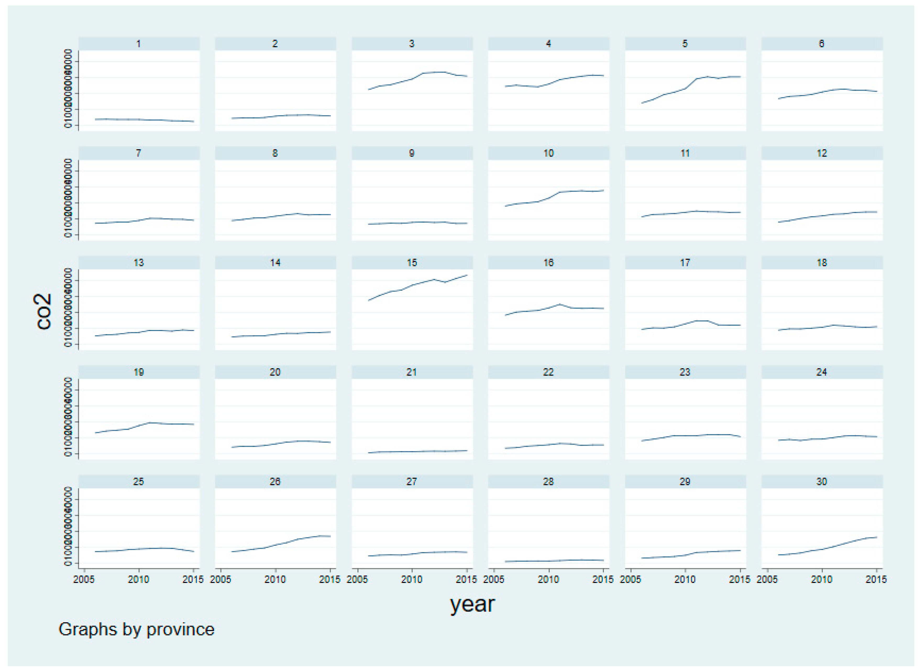
4.1. Evolving Temporal–Spatial Trends of Carbon Emissions

Table 2. Carbon emissions of each province (10⁴ t).

Province (Code)	Max	Min	Std.Dev	Mean	Province (Code)	Max	Min	Std.Dev	Mean
Beijing (1)	3676.09	2229.41	486.74	3177.83	Henan (16)	24,926.65	18,113.67	1856.12	21,752.56
Tianjin (2)	6350.87	4239.85	831.02	5417.26	Hubei (17)	14,638.92	9249.13	1828.78	11,801.00
Hebei (3)	33,201.25	22,295.19	3919.16	28,942.54	Hunan (18)	11,819.73	8742.85	939.25	10,379.75
Shanxi (4)	31,434.07	24,067.84	3066.53	27,505.21	Guangdong (19)	19,385.35	12,922.21	2317.05	16,806.16
Inner Mongolia (5)	30,365.01	13,914.11	6467.47	24,208.61	Guangxi (20)	7706.48	4003.39	1455.02	6113.58
Liaoning (6)	22,631.06	16,678.23	2041.69	20,274.14	Hainan (21)	1700.93	519.37	351.68	1228.91
Jilin (7)	10,203.68	7041.50	1145.28	8749.98	Chongqing (22)	6273.47	3368.32	938.74	5047.56
Heilongjiang (8)	13,105.08	8776.32	1474.13	11,366.73	Sichuan (23)	11,892.03	8046.15	1293.68	10,689.32
Shanghai (9)	7869.95	6647.88	431.61	7240.44	Guizhou (24)	11,289.85	8148.24	1182.92	9703.65
Jiangsu (10)	27,646.59	17,952.31	3928.10	23,678.54	Yunnan (25)	9357.88	7161.40	839.92	8261.53
Zhejiang (11)	14,792.01	11,197.74	1068.90	13,528.30	Shaanxi (26)	16,903.70	7135.05	3807.18	12,171.28
Anhui (12)	14,199.01	7878.49	2268.89	11,761.87	Gansu (27)	6969.15	4380.02	998.22	5879.43
Fujian (13)	8872.28	5125.51	1336.80	7394.47	Qinghai (28)	1991.52	882.20	358.21	1441.74
Jiangxi (14)	7549.21	4497.82	1104.76	6133.28	Ningxia (29)	7733.67	2976.65	1890.62	5527.89
Shandong (15)	43,219.32	27,446.43	5065.92	36,422.74	Xinjiang (30)	16,152.10	5023.51	4142.08	10,104.09
East provinces	43,219.33	519.37	11,136.55	14,919.21	West provinces	30,365.01	882.20	6221.69	9013.52
Middle provinces	31,434.07	4497.82	6939.46	1,094,503.67	30 provinces	43,219.32	519.3718	8930.02	12,423.68

shows the maximum value, minimum value, standard deviation, and mean value of carbon emissions in 30 provinces in mainland China from 2006 to 2015. The minimum value appeared in Hainan Province in 2006, which is only 5.1937 million tons. The maximum value appeared in Shandong Province in 2015, which is up to 432.1932 million tons. The top five provinces in mean value are Shandong, Hebei, Shanxi, Inner Mongolia, and Jiangsu. The last five provinces are Tianjin, Chongqing, Beijing, Qinghai, and Hainan. Among them, carbon emissions in Shandong is 364 million tons, but carbon emissions in Hainan is only 12.2891 million tons, the former is 29.64 times of the latter one. Each of the top four provinces of carbon emissions has more than 300 million tons of carbon emissions, while all the last three provinces are less than 40 million. This shows that the distribution of carbon emissions across each province is uneven.

To further analyze the regional differences, the 30 provinces are divided into three regions according to official documents: East, Center and West. The eastern region includes: Beijing, Tianjin, Hebei, Liaoning, Shanghai, Jiangsu, Zhejiang, Fujian, Shandong, Guangdong and Hainan these 11 provincial administrative units; the central region includes 8 provinces: Shanxi, Jilin, Heilongjiang, Anhui, Jiangxi, Henan, Hubei, and Hunan; the western region includes Inner Mongolia, Guangxi, Chongqing, Sichuan, Guizhou, Yunnan, Shaanxi, Gansu, Qinghai, Ningxia, Xinjiang these 11 provinces. The results show that in those three regions, the provinces in western region had the lowest mean value, that is 90.1352 million tons and the lowest standard deviation of 6221.69. The provinces in central region have the highest mean value of 10.9450367 billion tons, with a standard deviation of 6939.46, while the eastern provinces have a mean value of 149.1921 million tons of carbon emissions, but the standard deviation is as high as 11,136.55. This shows that the mean value of carbon emissions of each province in the western region is small and the difference of each province is also small. The central region is a high-emission region, although the mean value in eastern region is smaller than that of the central region, the difference between among the provinces is large. In the eastern region, there are not only high-emission provinces such as Shandong, Hebei, and Jiangsu, but also small-emission provinces such as Tianjin, Beijing, and Hainan. In the western region, there are not only high-emission provinces such as Inner Mongolia, but also the low-emission provinces such as Qinghai, which leads to great heterogeneity of carbon emissions among provinces and regions in China. According to the calculation results, we can know that the total mean value of 30 provinces across the country is 124.2368 million tons, and the standard error of the whole country is greater than that of the western region and the central region, but smaller than that of the eastern region, which further indicates that the difference of the provinces in eastern region is the most obvious.

Figure 1 shows the evolving temporal–spatial trends of carbon emissions in each province from 2006 to 2015, in which the provincial code is consistent with Table 2, 1 represents the Beijing and 30 represents the Xinjiang province. It can be seen from the figure that there are three main forms of carbon emissions evolution trend in the 30 provinces: linear growth type, inverted U shape and “no obvious fluctuation” type. Shandong Province (the code is 5), which ranks the first place in terms of carbon emissions, and the Inner Mongolia (the code is 15) ranks the fourth place, showed an overall trend of increasing and a kind of linear growth trend year by year, it only decreased in 2013, and then increased rapidly. Some provinces with high emissions showed a gradual increase trend from 2006 to 2010 but showed a gradual decrease trend from 2011 to 2015, such as the provinces with code number of 3 and 10 (Hebei Province and Jiangsu Province). The last five provinces, whose code numbers are 1, 2, 21, 22, 28, with smaller carbon emissions and a small change of variation in each year. It is found that there are 20 provinces that have less carbon emissions in 2015 than in 2014. This has led to a linear increase in China’s overall carbon emissions from 2006 to 2014, but it decreased suddenly in 2015. The time evolution trend of each province in the three regions is also quite different, in the eastern region, there are not only the provinces with liner growth trend (Shandong), but also provinces that exhibit a “inverted U shape” trend (Hebei), there are still the provinces with low emissions and small obvious fluctuation, such as Tianjin, Beijing and Hainan. In the western region, there are not only provinces that show liner growth trend, such as Inner Mongolia, Shaanxi, Xinjiang, but also the provinces without obvious fluctuation such as Qinghai, which leads to the heterogeneity of the evolution trend of carbon emissions among provinces and regions in China.

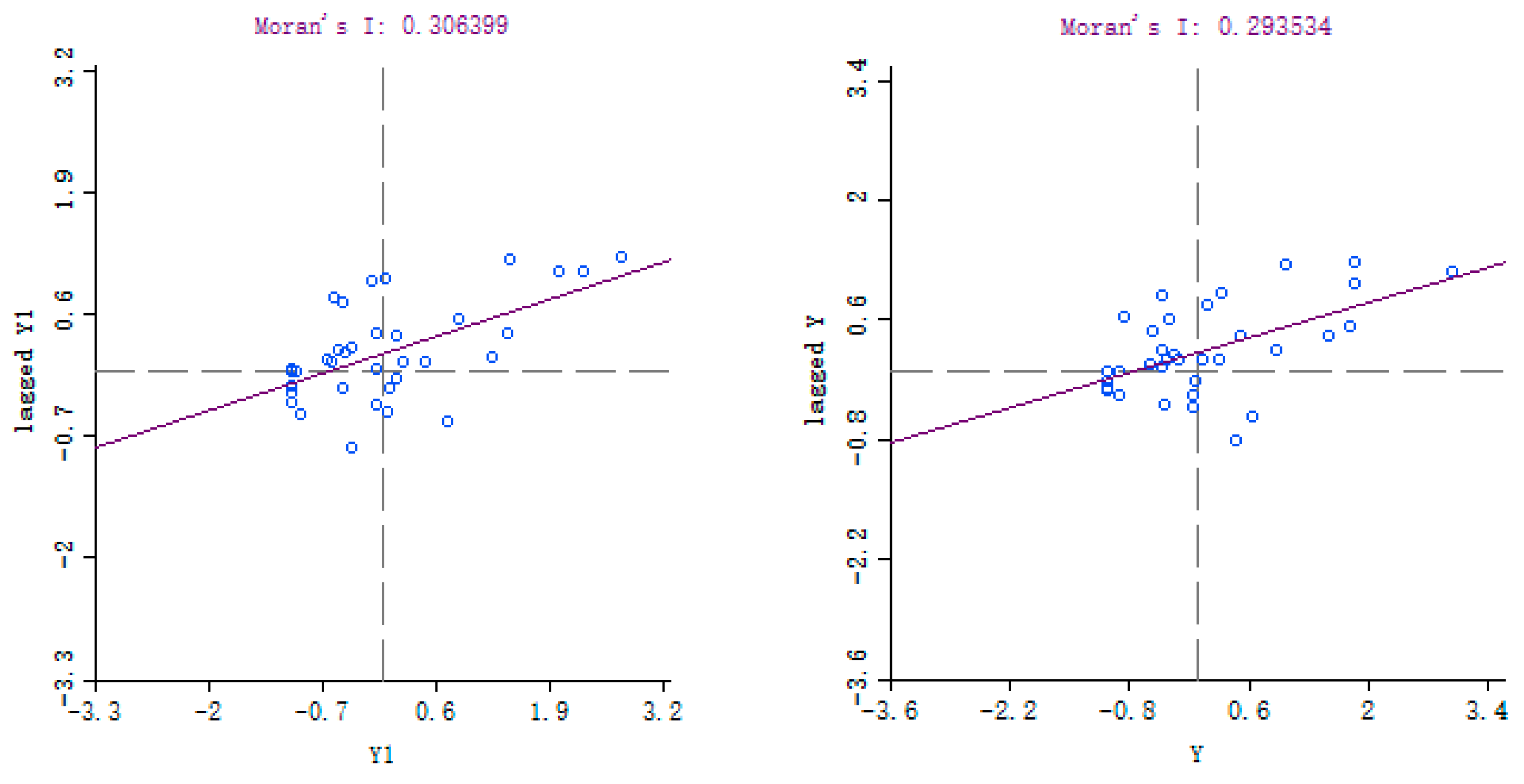
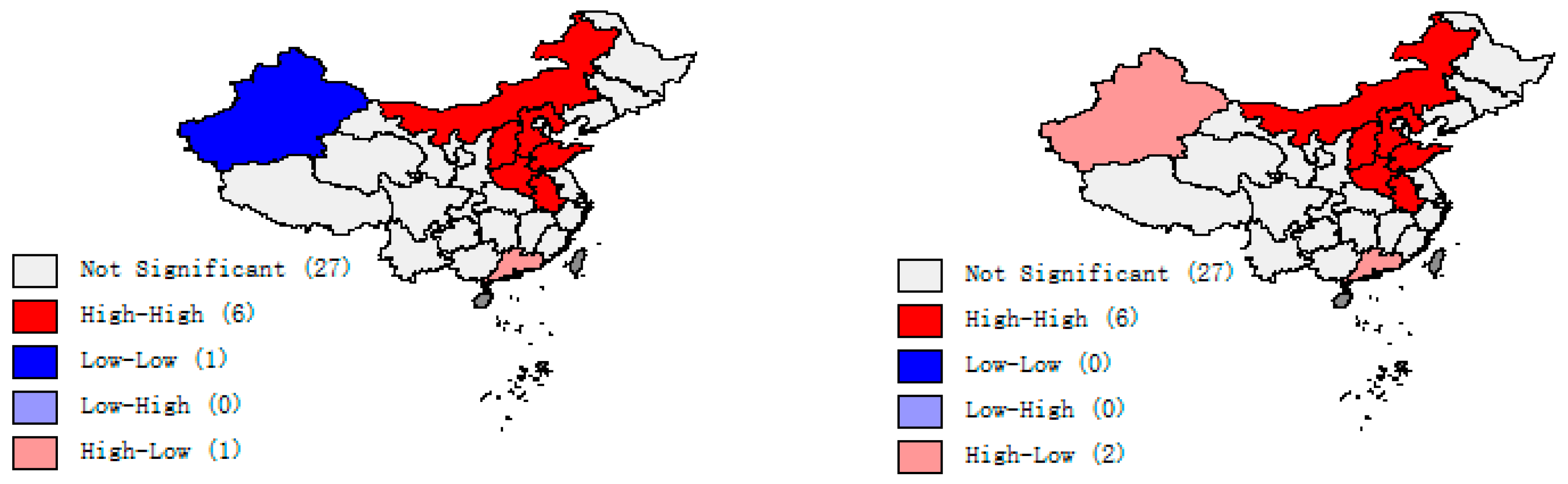
4.2. Spatial Correlation of Carbon Emissions

Table 3. The Moran’s I index of carbon emissions (2006–2015).

Year	Moran’s I	p-Value	Z-Value	Year	Moran’s I	p-Value	Z-Value
2006	0.3064	0.001	4.167	2011	0.3281	0.002	4.861
2007	0.3154	0.001	4.316	2012	0.3224	0.001	4.538
2008	0.3268	0.002	4.619	2013	0.3138	0.001	4.276
2009	0.3382	0.001	4.807	2014	0.3052	0.001	4.032
2010	0.3431	0.002	5.007	2015	0.2935	0.001	4.008

shows that the Moran’s I index is positive, fluctuating in the range of 0.29–0.34, and shows a trend of first increasing and then decreasing. It shows an increasing trend from 2006 to 2010, with a slight decrease from 2011 to 2015. The value of p is less than 0.05, the value of Z is larger than 1.96. This suggests that there is a significant spatial positive correlation of carbon emissions in 30 provinces from 2006 to 2015.

Figure 2 presents Moran scatter plots of carbon emissions of 30 provinces in China in the year of 2006 and 2015. The figure shows that most of the provinces in China are in the first quadrant (“H-H”-type) and the third quadrant (“L-L”-type). In the scatter plots of 2006 and 2015, the provinces in the first and third quadrants accounted for 66.67% and 63.33% of all provinces. This indicates that most of the provinces in China have similar spatial aggregation characteristics with their neighboring provinces, the provinces with high carbon emissions intensity are surrounded by the neighboring provinces with high carbon emissions intensity, and the provinces with low carbon emissions intensity are surrounded by the neighboring provinces with low carbon emissions intensity. Compared with 2006, the number of provinces in the first quadrant increased in 2015, but the number of provinces in the third quadrant decreased and the degree of aggregation had been decreased slightly.

Because the provinces in the first quadrant have the homogenization characteristics of “high-high” aggregation, and carbon emissions of these provinces and surrounding provinces are relatively large, therefore, this paper sets them as “priority emission reduction areas”. The provinces in the third quadrant show the homogenization characteristics of “low-low” aggregation, so this paper calls it as the “emission reduction buffer areas”. However, the provinces in the second quadrant have lower carbon emissions than those in the surrounding areas, so it is necessary to prevent the pollution from spreading into the surrounding provinces, so this paper regards it as the “emission reduction observation area”. In addition, the provinces in the fourth quadrant, whose own carbon emissions is significantly higher than that of the surrounding provinces, so this paper regards them as the “key emission reduction areas”. Although all the four quadrants in Figure 2 have the provincial distribution, the provinces that pass the significance test are the provinces that really show the characteristics of aggregation.

The LISA significance map can clearly show the regions with strong autocorrelation in local space, as shown in Figure 3. In 2006, there were 6 provinces showed “H-H” Aggregation characteristics, namely Shandong, Hebei, Shanxi, Inner Mongolia, Henan, and Anhui. Among them, the first four provinces are also the top four provinces with higher carbon emissions. Xinjiang is a “L-L” province, it is the province with low carbon emissions together with its surrounding provinces, which in 2006 were less economically developed provinces in the western region. Guangdong province belongs to “H-L”-type, for its own carbon emissions is significantly higher than that of neighboring provinces, and the degree of economic development is also higher than that of neighboring provinces.

In 2015, there were still six “H-H” provinces, which is the same as in 2006. Guangdong is still a “H-L” province, but the different situation is that Xinjiang has changed from the “L-L”-type to “H-L”-type. This is closely related to the development of energy and industrialization in Xinjiang. Xinjiang is a big energy province, bordering the big energy countries such as Central Asia and Russia, except that its energy consumption is also dominated by traditional fossil energy. In recent years, the province has been in a leapfrog stage of development, the industrialization process has also been accelerated, thus resulting in increased energy consumption and carbon emissions. Therefore, the Inner Mongolia, Shanxi, Shandong, Hebei, Henan, Anhui should be regarded as “priority emission reduction areas”, Xinjiang and Guangdong should be taken as the “key emission reduction areas”. In the future, we should assign the emission reduction tasks according to the socio-economic conditions of the provinces and adjust the emission reduction strategies at any time according to the changes in the actual situation. There are no “L-H”-type provinces in 2006, there are neither the “L-L”-type nor the “L-H” provinces in 2015, which indicates that the task of reducing carbon emissions in Chinese provinces is still very arduous, and it is necessary to effectively control the increase of carbon emissions.

4.3. Influencing Factors of Carbon Emissions

4.3.1. Comparative Analysis of the Results of Three Panel Models

The least square method is usually used to estimate general panel data, but this method may lead to the partial or invalid estimation results of the spatial econometric model. Therefore, the maximum likelihood method is used to estimate the parameters of the SLM and SEM models [39]. In this paper, the panel data of 30 provinces in China from 2006 to 2015 are selected for empirical analysis. The data are analyzed by using the traditional panel data regression analysis method firstly, from the estimation results of Hausman test, the fixed effect is the most suitable regression model. Moreover, when the data analysis is limited to some specific individuals, the fixed effect model is also a better choice [40]. Therefore, this paper applies the fixed effect model, that is the model 1. Then we analysis the SLM and SEM by MATLAB software. It is used to estimate the non-fixed effect, space-fixed effect, time-fixed effect, and time-space-fixed effect respectively. However, from the results of the four models, the goodness of fit and logarithmic likelihood value of the spatial fixed effect model are the highest, which is the most suitable model, so we only list the results of the spatial fixed effect model in this paper that is the Model 2 and Model 3 in

Table 4. The results of three panel models.

	Ordinary Panel Models	SLM	SEM
	Model1	Model 2	Model3
lnP (pop)	0.247 **	0.233 **	0.263 **
lnA (pgdp)	0.433 ***	0.732 ***	0.721 ***
lnT (technology)	−0.025 *	−0.028 *	−0.026 *
lnER	−0.034 *	−0.031 **	−0.032 **
lnEC	0.102	0.416 **	0.411 **
lnIL	0.007 *	0.006 **	0.008 **
lnUL	0.008	0.019 **	0.012 **
lnFDI	0.076	0.079	0.801
lnIFA	0.037 **	0.054 ***	0.072 ***
$\rho$		0.4786 **
$\lambda$			0.4626 *
$R^2$	0.663	0.684	0.673
Log likelihood	208.462	319.097	316.917

Note: ***, ** and * denote a significance of 1%, 5% and 10%.

. The results of these three models are compared and the best model is selected in the following text.

Model 1 does not consider the spatial correlation, only the population and per capita GDP. Technology level, government environmental governance input, industrial structure, and IFA have significant impact on carbon emissions; in addition, the population number, per capita GDP, industrial structure and IFA have positive promoting effects on the increase of carbon emissions. However, the technology level and government investment in environmental governance can significantly inhibit the increase of carbon emissions. The significance of technology level and government investment in environmental governance is lower than that of other factors. In the SLM, model 2 shows that the population number, per capita GDP, per unit of GDP energy consumption, industrial structure, urbanization rate, and IFA have significant positive impact on carbon emissions, and the technology level as well as the government investment in environmental governance have significant inhibitory effects on carbon emissions. The significance of per capita GDP and IFA were higher than other factors. In the SEM, model 3 shows that the population number, per capita GDP, energy consumption of per unit GDP, industrial structure, urbanization rate, IFA are all positively correlated with regional carbon emissions. Furthermore, the technical level and the government investment in environmental governance are negatively correlated with carbon emissions.

The results of model 2 and model 3 are basically consistent, but there is a big difference between them and model 1. Under the condition of SLM, $\rho$ is greater than 0 and it has passed the significance test; under the condition of SEM, $\lambda$ is greater than 0 and it has passed the significance test, which shows that the regional carbon emissions has obvious spatial “spillover effect”, spatial factors play an important role in regional carbon emissions. Therefore, the time effect and space effect must be considered when analyzing the influencing factors. To select an optimal model, the relevant parameters of the SLM and the SEM are further tested below.

4.3.2. Selection of Optimal Model and the Analysis of Result

By analyzing the values of Lm-lag and Lm-error and testing the spatial correlation, we can select a more suitable spatial econometric model. Lm-lag and Lm-error are used to test the SLM and the SEM respectively, if only one of them is significant, then we can choose the corresponding model directly. If both are significant, the values of Robust Lm-lag and Robust Lm-error needed to be observed. If the former one is significant, then the SLM is chosen, and if the latter one is more significant, then the SEM is selected. The testing results of the spatial correlation are shown in

Table 5. Spatial correlation Lm test.

Lm-Lag	Lm-Error	Robust Lm-Lag	Robust Lm-Error
98.634 *** (0.000)	75.381 *** (0.000)	36.806 *** (0.000)	23.614 (0.137)

Note: The number in parenthesis is p-value. *** p < 0.01.

.

Table 5 shows that both results of Lm-lag and Lm-error are significant. However, as for Robust Lm-lag and Robust Lm-error, only the former one is significant. Therefore, the fixed effect model under the condition of SLM is the optimal model. In model 2, FDI has no significant effect on carbon emissions. population pressure, degree of affluence, energy intensity, industrial structure, UL, fixed asset investment can significantly promote the increase of regional carbon emissions. However, the technical level and the ER have the remarkable inhibition function to the increase of carbon emissions. Among the positive influencing factors, the significance of per capita GDP and IFA are higher than that of other factors. In the negative influencing factors, the significance of technical level is lower than that of environmental supervision. This shows that the current carbon emissions in provinces of China are mainly caused by economic development and internal investment, and there is no “pollution paradise” effect of FDI. The working effect of carbon emission reduction is mainly driven by government investment in environmental governance; at the same time, the driving force of technical progress is relatively small. overall, the coefficients of technical level and ER are very small, their significance is less than per capita GDP and the IFA. This suggests that the factors that contribute to the increase in carbon emissions play a stronger role than those inhibiting factors, and carbon emission reduction work in China is a very difficult task.

5. Conclusions and Policy Implications

5.1. It Is Necessary to Carry Out the Work of Reducing Carbon Emissions in a Targeted Way

Overall, there is a great heterogeneity in the evolving temporal–spatial trends of carbon emissions among provinces and regions in China. The mean values of carbon emissions in each province in the western region are small and the differences among the provinces are also small. The central region is a high-emission region, and the mean value of the eastern region is between the other two parts, but the standard deviation is the largest. Therefore, emphasis should be placed on carbon emission reduction in the central region and implementing the differentiated emission reduction strategies in the eastern region. There is a great difference in carbon emissions between provinces inside the region; at the same time, the trend of spatial and temporal evolution shows various forms, such as “linear growth”, “inverted U shape” and “no obvious fluctuation”. Therefore, it is necessary to carry out work of reducing carbon emissions according to the actual situation of each province. In areas with high-emission and “linear growth” trend, measures should be taken quickly to effectively curb its growth trend. In the “inverted U” regions, carbon emissions should be prevented from rebounding.

5.2. Confirm the Priority Emission Reduction Areas and Prevent the Situation Worsening

There are significant positive spatial correlation and aggregation characteristics of carbon emissions in China. The number of “H-H”-type provinces is relatively large, such as Shandong, Hebei, Shanxi, Inner Mongolia, Henan, Anhui; all of these provinces and their surrounding provinces have very high carbon emissions, so they should be set up as the priority emission reduction areas and take a positive attitude towards the work of carbon emission reduction. “H-L”-type provinces, such as Guangdong Province, whose potential of emission reduction is great, can be regarded as key emission reduction areas to prevent emissions from spreading to the surrounding areas. It should be noted that the characteristics of regional aggregation would change with the passage of time, for example, the transformation from “L-L”-type to “H-L”-type in Xinjiang province. Therefore, it is necessary to adjust strategies in time according to the development trend of each province, to prevent the situation worsening.

5.3. It Is Necessary to Adjust the Economic Structure, Promote Technical Progress and Strengthen Supervision

Population pressure, degree of affluence, energy intensity, industrial structure, UL, IFA all can significantly promote the increase of regional carbon emissions. The technical level and the ER of government have an obviously inhibited function on the increase of carbon emissions; in addition, foreign investment has no significant impact on carbon emissions. This shows that carbon emissions of 30 provinces in China are closely related to their own economic and social development. In the rapid process of industrialization and urbanization, the population needs to be fed and energy consumption is increasing. While China is creating an economic miracle, its carbon emissions continue to increase. Therefore, it is necessary to further relieve the environmental pressure caused by population growth, economic development, and energy consumption by strengthening environmental supervision and regulation as well as promoting technical progress.

References

1. Le Quéré, C.; Andrew, R.M.; Canadell, J.G.; Sitch, S.; Korsbakken, J.I.; Peters, G.P.; Manning, A.C.; Boden, T.A.; Tans, P.P.; Houghton, R.A.; et al. Global carbon budget. Earth Syst. Sci. Data 2016, 8, 605–649. [Google Scholar] [CrossRef]
2. Le Quéré, C.; Andrew, R.M.; Friedlingstein, P.; Sitch, S.; Pongratz, J.; Manning, A.C.; Korsbakken, J.I.; Peters, G.P.; Canadell, J.G.; Jackson, R.B.; et al. Global Carbon Budget 2017. Earth Syst. Sci. Data 2018, 10, 405–448. [Google Scholar] [CrossRef] [Green Version]
3. Acaravci, A.; Ozturk, I. On the relationship between energy consumption, CO2 emissions and economic growth in Europe. Energy 2010, 35, 5412–5420. [Google Scholar] [CrossRef]
4. Ding, Y.; Li, F. Examining the effects of urbanization and industrialization on carbon dioxide emission: Evidence from China’s provincial regions. Energy 2017, 125, 533–542. [Google Scholar] [CrossRef]
5. Pao, H.T.; Tsai, C.M. Multivariate Granger causality between CO2 emissions, energy consumption, FDI (foreign direct investment) and GDP (gross domestic product): Evidence from a panel of BRIC (Brazil, Russian Federation, India, and China) countries. Energy 2011, 36, 685–693. [Google Scholar] [CrossRef]
6. Yin, J.; Zheng, M.; Chen, J. The effects of environmental regulation and technical progress on CO2, Kuznets curve: An evidence from China. Energy Policy 2015, 77, 97–108. [Google Scholar] [CrossRef]
7. Tobler, W.R. A computer movie simulating urban growth in the Detroit region. Econ. Geogr. 1970, 46 (suppl. 1), 234–240. [Google Scholar] [CrossRef]
8. Chuai, X.; Huang, X.; Wang, W.; Wen, J.; Chen, Q.; Peng, J. Spatial econometric analysis of carbon emissions from energy consumption in China. J. Geogr. Sci. 2012, 22, 630–642. [Google Scholar] [CrossRef]
9. Keller, W. Geographic Localization of International Technology Diffusion. Am. Econ. Rev. 2002, 92, 120–142. [Google Scholar] [CrossRef] [Green Version]
10. Solomon, S.; Qin, D.; Manning, M.; Chen, Z.; Marquis, M.; Averyt, K.B.; Tignor, M.; Miller, H.L. Contribution of Working Group to the Fourth Assessment Report of the Intergovernmental Panel on Climate Change; IPCC: Geneva, Switzerland, 2007. [Google Scholar]
11. Quadrelli, R.; Peterson, S. The energy climate challenge: Recent trends in CO emissions from fuel combustion. Energy Policy 2007, 35, 5938–5952. [Google Scholar] [CrossRef]
12. Raupach, M.R.; Marland, G.; Ciais, P.; Le Quéré, C.; Canadell, J.G.; Klepper, G.; Field, C.B. Global and regional drivers of accelerating CO2 emissions. Proc. Natl. Acad. Sci. USA 2007, 104, 10288–10293. [Google Scholar] [CrossRef] [PubMed]
13. Choi, K.H.; Ang, B.W. A time-series analysis of energy-related carbon emissions in Korea. Energy Policy 2001, 29, 1155–1161. [Google Scholar] [CrossRef]
14. Hammond, G.P.; Norman, J.B. Decomposition analysis of energy-related carbon emissions from UK manufacturing. Energy 2012, 41, 220–227. [Google Scholar] [CrossRef] [Green Version]
15. Wang, S.; Fang, C.; Wang, Y.; Huang, Y.; Ma, H. Quantifying the relationship between urban development intensity and carbon dioxide emissions using a panel data analysis. Ecol. Indic. 2015, 49, 121–131. [Google Scholar] [CrossRef]
16. Dhakal, S. Urban energy use and carbon emissions from cities in China and policy implications. Energy Policy 2009, 37, 4208–4219. [Google Scholar] [CrossRef]
17. Huang, B.; Meng, L. Convergence of per capita carbon dioxide emissions in urban China: A spatio-temporal perspective. Appl. Geogr. 2013, 40, 21–29. [Google Scholar] [CrossRef]
18. Wang, S.; Fang, C.; Wang, Y. Spatiotemporal variations of energy-related CO2 emissions in China and its influencing factors: An empirical analysis based on provincial panel data. Renew. Sustain. Energy Rev. 2016, 55, 505–515. [Google Scholar] [CrossRef]
19. Ebohon, O.J.; Ikeme, A.J. Decomposition analysis of CO2 emission intensity between oil producing and non-oil-producing sub-Saharan African countries. Energy Policy 2006, 34, 3599–3611. [Google Scholar] [CrossRef]
20. Jayanthakumaran, K.; Verma, R.; Liu, Y. CO2 emissions, energy consumption, trade and income: A comparative analysis of China and India. Energy Policy 2012, 42, 450–460. [Google Scholar] [CrossRef]
21. Pao, H.T.; Yu, H.C.; Yang, Y.H. Modeling the CO2 emissions, energy use, and economic growth in Russia. Energy 2011, 36, 5094–5100. [Google Scholar] [CrossRef]
22. Pao, H.T.; Tsai, C.M. Modeling and forecasting the CO2 emissions, energy consumption, and economic growth in Brazil. Energy 2011, 36, 2450–2458. [Google Scholar] [CrossRef]
23. Ozcan, B. The nexus between carbon emissions, energy consumption and economic growth in Middle East countries: A panel data analysis. Energy Policy 2013, 62, 1138–1147. [Google Scholar] [CrossRef]
24. Li, H.; Mu, H.; Zhang, M.; Li, N. Analysis on influence factors of China’s CO emissions based on Path-STIRPAT model. Energy Policy 2011, 39, 6906–6911. [Google Scholar] [CrossRef]
25. Haseeb, M.; Hassan, S.; Azam, M. Rural-urban transformation, energy consumption, economic growth, and CO2 emissions using STRIPAT model for BRICS countries. Environ. Prog. Sustain. Energy 2017, 36, 523–531. [Google Scholar] [CrossRef]
26. Shahbaz, M.; Loganathan, N.; Muzaffar, A.T.; Ahmed, K.; Jabran, M.A. How urbanization affects CO2 emissions in Malaysia? The application of STIRPAT model. Renew. Sustain. Energy Rev. 2016, 57, 83–93. [Google Scholar] [CrossRef]
27. Wang, Z.; Yin, F.; Zhang, Y.; Zhang, X. An empirical research on the influencing factors of regional CO2 emissions: Evidence from Beijing city, China. Appl. Energy 2012, 100, 277–284. [Google Scholar] [CrossRef]
28. Li, B.; Liu, X.; Li, Z. Using the STIRPAT model to explore the factors driving regional CO2, emissions: A case of Tianjin, China. Nat. Hazards 2015, 76, 1667–1685. [Google Scholar] [CrossRef]
29. Wang, C.; Wang, F.; Zhang, X.; Yang, Y.; Su, Y.; Ye, Y.; Zhang, H. Examining the driving factors of energy related carbon emissions using the extended STIRPAT model based on IPAT identity in Xinjiang. Renew. Sustain. Energy Rev. 2017, 67, 51–61. [Google Scholar] [CrossRef]
30. Li, H.; Mu, H.; Zhang, M.; Gui, S. Analysis of regional difference on impact factors of China’s energy-related CO2 emissions. Energy 2012, 39, 319–326. [Google Scholar] [CrossRef]
31. Zhao, W.; Niu, D. Prediction of CO2 Emission in China’s Power Generation Industry with Gauss Optimized Cuckoo Search Algorithm and Wavelet Neural Network Based on STIRPAT model with Ridge Regression. Sustainability 2017, 9, 2377. [Google Scholar] [CrossRef]
32. Lin, B.; Liu, K. Using LMDI to Analyze the Decoupling of Carbon Dioxide Emissions from China’s Heavy Industry. Sustainability 2017, 9, 1198. [Google Scholar]
33. Hamit-Haggar, M. Greenhouse gas emissions, energy consumption and economic growth: A panel cointegration analysis from Canadian industrial sector perspective. Energy Econ. 2012, 34, 358–364. [Google Scholar] [CrossRef]
34. Wu, C.; Li, G.; Yue, W.; Lu, R.; Lu, Z.; You, H. Effects of endogenous factors on regional land-use carbon emissions based on the Grossman decomposition model: A case study of Zhejiang Province, China. Environ. Manag. 2015, 55, 467–478. [Google Scholar] [CrossRef] [PubMed]
35. Xu, H. Spatial and econometric analysis of spatial dependence, carbon emissions and per-capita Income. China Popul. Resour. Environ. 2012, 22, 149–157. [Google Scholar]
36. Anselin, L. Local indicators of spatial association-LISA. Geogr. Anal. 1995, 27, 93–115. [Google Scholar] [CrossRef]
37. Ehrlich, P.R.; Holdren, J.P. Impact of Population Growth. Science 1971, 171, 1212–1217. [Google Scholar] [CrossRef] [PubMed]
38. Dietz, T.; Rosa, E.A. Rethinking the Environmental Impacts of Population, Affluence and Technology. Hum. Ecol. Rev. 1994, 2, 277–300. [Google Scholar]
39. Han, N.; Yu, W. Spatial Characteristics and Influencing Factors of Industrial Waste Gas Emission in China. Sci. Geogr. Sin. 2016, 36, 196–203. [Google Scholar]
40. Elhorst, J.P. Specification and estimation of spatial panel data models. Int. Reg. Sci. Rev. 2003, 26, 244–268. [Google Scholar] [CrossRef]
Figure 1. Evolving temporal–spatial trends of each province (2006–2015).
Sustainability 10 02809 g001
Figure 2. Moran scatter plots of CO2 of 30 provinces in China in 2006 (left) and 2015 (right).
Sustainability 10 02809 g002
Figure 3. LISA agglomeration map of CO2 in 2006 (left) and 2015 (right).
Sustainability 10 02809 g003